Assessment of the Modeling of Demand Response as a Dispatchable Resource in Day-Ahead Hydrothermal Unit Commitment Problems: The Brazilian Case

Abstract

Modern power systems have experienced large increases in intermittent and non-dispatchable sources and a progressive reduction in the size of hydro reservoirs for inflow regularization. One method to mitigate the high uncertainty and intermittency of the net load is by Demand Response (DR) mechanisms, to allow a secure and reliable system dispatch. This work applied a mixed integer linear programming formulation to model DR as a dispatchable resource in the day-ahead hydrothermal scheduling problem, taking into account minimum load curtailment constraints, minimum up/down load deduction times, as well as piecewise linear bid curves for load shedding in eligible loads. The methodology was implemented in the official model used in Brazil and tested in large-scale problems to obtain the optimal daily dispatch and hourly pricing. The results show the positive impact of dispatchable DR loads in cost reduction and in mitigating peak values of energy prices, even for predominantly hydro systems, helping to preserve the reservoir levels and increasing the security of the supply in the future.

1. Introduction

Modern power systems have experienced a large increase in intermittent and non-dispatchable sources–such as wind and solar plants, as well as increasing difficulty in building new hydro plants with large reservoirs for inflow regularization. Therefore, many methods of mitigating the high uncertainty and intermittency of the net load have been proposed in power generation systems to allow a secure and reliable system dispatch in power generation systems. Some resources work on the generation side of the grid, such as pumped storage power plants [1], energy storage devices [2], and, more recently, green hydrogen technology [3]. In such cases, the aim is to store the excess of renewable generation—wind and solar plants in offpeak hours, where energy demand and prices are low, to use them in hours with peak energy and prices, thus yielding a smoother net load pattern and a reduction in generation costs.

Another method of mitigating the high volatility of prices and net load is Demand Side Management (DSM) mechanisms [4], which involves encouraging consumers to reduce their energy consumption without leaving aside the comfort or stimulating a gradual reduction in consumption by performing the same activities. In terms of the power system operation, the main goal is to motivate a shift in the load consumption behaviour of consumers from peak hours to low level hours, or even a load reduction in exchange for lower energy prices.

In general, DSM can be divided in two main categories: Energy Efficiency (EE) and Demand Response (DR). The main purpose of EE is to reduce energy net consumption while accomplishing the same tasks, while DR refers to load profile adjustments, as, for example, load shifting and load shedding, which are driven by market incentives [5]. An extensive literature survey is provided, for example, in [6], which presents, among other things, recent developments of the DSM of electrical power systems, as well as in [7], which shows a survey on methods for optimization of the demand response. 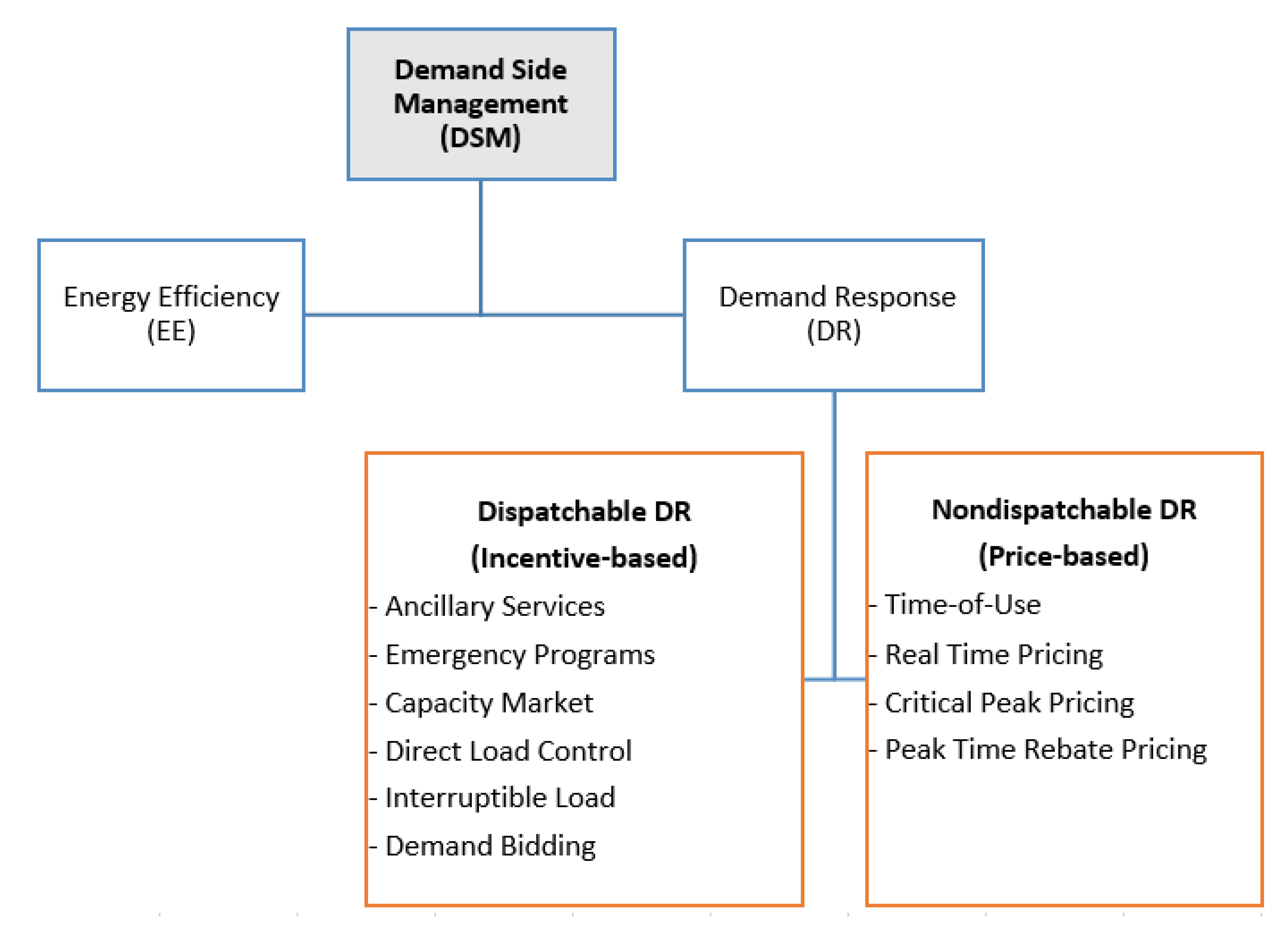Figure 1 presents the main categories of DSM, separated by EE and DR, which represent only some of the many existing DSM programs in the energy markets around the world [8,9].

DSM mechanisms are widely considered in several energy markets, such as the US, Spain, and France [10,11], and represent an important tool to provide adequate expansion of the electricity system as well as to help increasing the reliability and security of the energy supply system in many countries. The work [12] studies the application of DR in security constrained problems, while [13] assesses the application of DR in the context of profit maximization in electricity markets. In [14], some methodological and practical aspects of the inclusion of DR in energy optimization problems are discussed.

Contributions of This Work

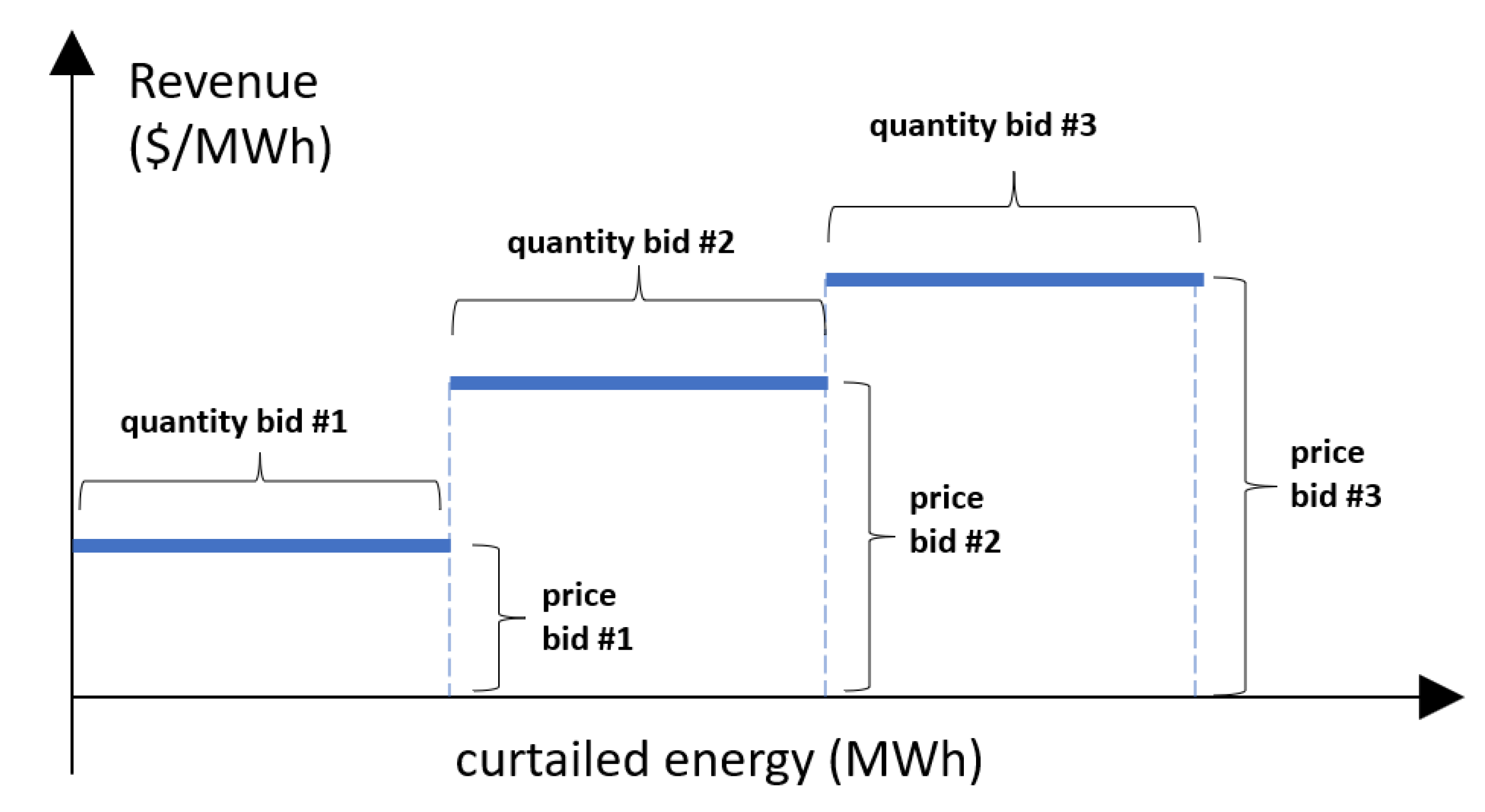
This work presents a thorough and realistic analysis of a mixed integer linear programming (MILP) formulation to model DR as a dispatchable resource, taking into account minimum load curtailment constraints, minimum up/down load deduction times, as well as piecewise linear bid curves for load shedding in eligible loads. Although the situation of demand retrieving the decreased consumption in later hours is an important analysis, this possibility was not considered in this work.

The methodology was implemented in the network-constrained hydrothermal unit commitment model named DESSEM, which is officially applied in Brazil for the day-ahead scheduling and hourly price setting [15]. In this sense, the contributions of this work are twofold: (i) to show the benefits of the application of DR programs even in predominantly hydro systems, by assessing the impact on energy prices and generation cost in real and official cases of day-ahead scheduling and pricing in Brazil. To the best of the authors’ knowledge, the few works that apply DR models to generation scheduling problems are restricted to pure thermal systems or to hydrothermal systems with a configuration much smaller and/or a representation of hydro, thermal, or network constraints less accurate as compared to [15]. The work [16] studied the hydrothermal generation scheduling with the inclusion of pumped storage-hydraulic units with DSM. In [17], an optimization model is proposed to smooth frequent local load fluctuations, and [18] studied the minimization of wind energy curtailment by scheduling DR, in such a way that higher values of demand match high wind generation values. The work [19] proposes an integrated stochastic scheduling model to dispatch resources considering both gas operation and the demand side to meet renewable energy intermittence; (ii) to present a MILP-based DR model that is able to provide results in reasonable CPU times in a real large-scale system, with over 160 hydro plants and 12,000 transmission lines, and taking into account 60 DR units grouped in 4 aggregators. The results assessed the amount of reduction in operational costs and the positive impact in mitigating peak values of energy prices, as well as reducing hydro generation, helping to preserve the reservoir levels.

2. Demand Response Programs

According to the International Energy Agency (IEA), DR programs have the potential to substantially improve power market flexibility and efficiency, delivering a range of benefits including more efficient market clearings, lower system prices, a decrease in peaking plant investment requirements, and greater flexibility with the potential to improve power system security [20].

The participation of several customer classes (residential, industrial, commercial, and transportation) in DR programs, which is facilitated by the large penetration of smart meters, combined with the high requirement for energy, have made the DR market in USA the largest in the world. According to the Federal Energy Regulatory Commission’s (FERC) 2019 report [10], in 2018, the USA had a participation in DR programs of around 29.7 GW among its System Operators (SO), representing 6.0% of the average peak load.

In Europe, many countries had already adopted consumer policy to be included as a mechanism to mitigate peak demand and delay the system expansion. France has consolidated DR mechanisms, such as balance mechanisms, capacity markets, among others, and had a total share in DR market in 2018 of around 48.9 GWh [21]. DR mechanisms in Spain are mostly composed of real-time pricing and interruptibility programs, where the latter is aimed at emergency situations when energy supply is insufficient to meet demand, and had a capacity to a reduce peak hour demand of 2000 MW in 2017 [11]. Norway encouraged specific programs aimed at delaying network expansion with the following results: a 10% reduction in peak demand in Oslo, increased knowledge about consumer behavior, and model development for DSM mechanisms [22].

DR mechanisms are structured in different regions of the world. In [23], an overview of the demand reaction in developing countries such as Chile and Colombia is presented. The DR market in countries such as Japan, China, and North Korea, as well as continents such as Africa and Oceania, has an extensive survey carried out in [24], indicating, in addition to the current panorama, the main barriers for introduction of DR programs in these regions. A study of the DR programs associated with renewable energies was analysed in [25] to explore an appropriate instrument to help system operators considering the increase in sustainability of worldwide electrical systems.

As can be seen in the DR literature and illustrated by Figure 1, DR programs can be proposed mainly in two ways [11,20]:

• dispatchable DR programs: allow the system operator to decide the dispatch of these loads based on bid curves for remuneration of loads according to the amount of load deduction. They are also known as an incentive-based DR program, in which consumers can receive payments to change their consumption patterns triggered by, for instance, high clearing market prices.
• non-dispatchable DR programs: where loads provide a long-term reduction in their pattern according to the behavior of prices (price-based DR program). Consumers can respond to wholesale market price variations or dynamic grid fees.

We considered in this study the first case, where the load can be deducted based on piecewise linear bid curves for load shedding in eligible loads.

3. Network-Constrained Hydrothermal Unit Commitment Problem (Nchtuc)

We considered a MILP-based NCHTUC problem on a cost minimization basis, whose formulation is summarized below. Due to space limitations, we refer to [15] for mathematical details and a richer description of constraints of the model, which is the one officially used for dispatch and price setting in Brazil and which was used in this work to model the DR as a dispatchable resource.

The objective Function (1) is to minimize total system operation costs Z, given by:

$$\begin{array}{cc}\hfill & minZ=\sum _{t=1}^T\left[\sum _{i=1}^{nt}(cs{t}_i^t(u_i^{t-1},u_i^t)+c{t}_i^{t}g{t}_i^t)+\sum _{i=1}^{NCI}c{i}_i^{t}Ei{m}_i^t-\right.\hfill \\ \hfill & \left.\sum _{i=1}^{NCE}c{e}_i^{t}Ee{x}_i^t\right]+{\alpha }_{FCF}(V_i+R_i)\hfill \end{array}$$

(1)

where $nt$ is the number of thermal units, each one with a generation $g{t}_i^t$ subject to linear or piecewise linear fuel costs given by $c{t}_i^t$. The “status-change” cost $cs{t}_i^t$ for thermal units comprises both startup and shutdown costs, which are a function of units status $u_t$. The terms $Ei{m}_i^t$ and $Ee{x}_i^t$ refer to imported and exported energy, respectively, with neighborhood systems, whose unitary prices are given by $c{i}_i^t$ ($c{e}_i^t$) for each of the NCI (NCE) import (export) contracts. The term ${\alpha }_{FCF}$ is the expected future operation cost, which depends on the vector of end storages $V_i$ and the amount of water in the river courses $R_i$ at the end of the time horizon (see [26] for details). Such a function is provided by the mid-term model [27].

The electrical network is represented by a linearized dc model, where reactive power is neglected and line flows are given by taking into account the first and second Kirchhoff laws, based on the reactance values for each transmission line, which are given data. The network model considered in this study includes, besides the energy balance constraints in each node, line flow limits in each transmission lines (2) as well as additional security constraints (3) [28].

$$\begin{array}{c}\hfill -\overline{f_l}\le \sum _{i=1}^{NB}{k}_{B_i^l}[g_i^t-d_i^t]\le \overline{f_l}\end{array}$$

(2)

$$\begin{array}{cc}\hfill & \underline{S{C}_i^t}\le \sum _{b\in SC{B}_i}{k}_{SC{B}_i^b}(g_b^t-d_b^t)+\sum _{l\in SC{L}_i}{k}_{SC{L}_i^l}{f}_l^t\le \overline{S{C}_i^t}\hfill \end{array}$$

(3)

where $f_l$ is the flow limit in each line l, $(g_i^t-d_i^t)$ represents generation and load in each bus, and $k_{B_i^l}$ are the participation factors that depend on the network topology. The parameters $SC{B}_i$, $SC{L}_i$, $k_{SC{B}_i^l}$, and $k_{SC{L}_i^l}$ of security constraints are provided by the system operator. The symbols with lower and upper bars in the left and right hand sides of (2) and (3) represent minimum and maximum values for the corresponding expressions. Additionally, additional security constraints given by tables or piece-wise linear functions are included in the model, as described in [15].

The hydro balance in the reservoirs is formulated as (4):

$$\begin{array}{cc}\hfill & V_i^t-V_i^{t-1}+{\zeta }^t\left[Q_i^t+S_i^t+Qe{v}_i^t+\sum _{j\in M{p}_i}Q{b}_j^t-\sum _{j\in J{p}_i}Q{p}_j^t\right.\hfill \\ \hfill & \left.-\sum _{j\in M_i}(Q_j^t+S_j^t)-\sum _{j\in Mt{v}_i}(Q_j^{t-\tau ji}+S_j^{t-{\tau }_{ji}})\right]\hfill \\ \\ \hfill & ={\zeta }^t\left[I_i^t-Qou{t}_i^t\right]\hfill \end{array}$$

(4)

where the known values are the natural inflows $I_i^t$ to reservoirs and water intakes $Qou{t}_i^t$ for other uses of water. Variables $Q_i^t$ and $S_i^t$ are the turbined (discharge) and spilled outflows, and $Qe{v}_i^t$ is the evaporation function of the reservoir, which is described in [15]. The sets $M{p}_i/J{p}_i$ indicate upstream/downstream pumping stations that take water from/to reservoir i, and $Mt{v}_i/M_i$ are the set of upstream plants j with/without water delay time to reservoir i, with a value of ${\tau }_{ji}$ in the first case. The factor ${\zeta }^t$ converts the average values of the variables in $m^3/s$ during interval t in the total amount of volume of water in interval t, ${hm}^3$, taking into account the duration of the interval.

The hydro generation $GH$ for plant i is a concave piecewise-linear function $GH(V,Q,S)$, whose expression is presented in [15], and the method of construction is presented in [29].

Thermal unit commitment constraints include: minimum generation (once turned on), startup/shutdown curves, minimum up/down times, maximum up and down ramp rates, and a detailed modeling of combined cycle units by a component-based model. The formulation of all these constraints is presented in [15].

Finally, a large number of operating constraints for the reservoirs are included in the model, as also detailed in [15].

4. Formulation of DR Constraints in the Nchtuc Problem

4.1. Bid Curves for Load Reduction

The bid curves for DR loads are price/quantity pairs, i.e., the revenue for load curtailment is a piecewise linear function of the amount of load reduction, as shown in Figure 2.

4.2. DR Constraints for Each Individual Load

The following constraints are enforced for DR loads:

• load reduction limits (once activated): the minimum and maximum DR reduction limits $(\underline{l_{D{R}_i}}$ and $\overline{l_{D{R}_i}})$ are defined in (5), where $u_{D{R}_i^t}$ is the status (1: activated; 0: disabled) for each DR load i in time t.

  $$\begin{array}{c}\hfill \overline{l_{D{R}_i}}.u_{D{R}_i^t}\le l_{D{R}_i^t}\le \underline{l_{D{R}_i}}.u_{D{R}_i^t}\end{array}$$

  (5)
• minimum on/off times for DR: once activated or disabled, expressions (6) and (7) impose the minimum times $To{n}_i/Tof{f}_i$, where the load reduction should remain on/off, respectively.

  $$\begin{array}{cc}\hfill & \sum _{k=t}^{t+To{n}_i-1}{u}_{D{R}_i^k}\ge To{n}_i.(u_{D{R}_i^t}-u_{D{R}_i^{t-1}})\hfill \end{array}$$

  (6)

  $$\begin{array}{cc}\hfill & \sum _{k=t}^{t+Tof{f}_i-1}(1-u_{D{R}_i^k})\ge Tof{f}_i.(u_{D{R}_i^{t-1}}-u_{D{R}_i^t})\hfill \end{array}$$

  (7)

4.3. Aggregator Constraints

Load aggregators were considered in this work due to their recognized importance for a secure stimulation and promotion of DR mechanism in a global context [30,31], since they can centralize many consumers to build a portfolio of DR load. In this sense, loads with small consumption can be aggregated and promote volumes that are large enough for their load to participate in the market [32].

Constraints for $NEC$ aggregators are mathematically represented in our model as special electrical constraints (EC), according to (8). Each constraint i indicates an aggregator with lower and upper limits $\underline{E{C}_i^t}$ and $\overline{E{C}_i^t}$ for time step t, and comprises a set $EC{L}_i$ of DR loads, each one contributing with a load reduction $D{R}_j^t$ and a participation factor $k_{EC,L_{i}j}$.

$$\begin{array}{cc}\hfill & \underline{{E{C}_i}^t}\le \sum {{}_{j\in EC{L}_i}}_{EC,L_{i}j}^{k}D{R}_j^t\le \overline{E{C}_i^t}\hfill \\ \\ \hfill & i=1,\cdots ,NEC;t=1,\cdots ,T.\hfill \end{array}$$

(8)

5. DR Characteristics

The study was applied to the real data for the hydrothermal Brazilian system and its pilot DR program. The system is divided into four subsystems: Southeast/Midwest, South, Northeast, and North. We considered 15 DRs (DR loads) per subsystem, each one with minimum and maximum reduction values (once activated) and Ton/Toff values given in

Table 1. Allowed reduction of each DR per subsystem.

Subsystem	Max.Reduction/Min.Reduction	Ton/Toff
Southeast/Midwest	108 MW/5 MW	1 h/1 h
South	31.5 MW/5 MW	1 h/1 h
Northeast	22.5 MW/5 MW	1 h/1 h
North	18 MW/5 MW	1 h/1 h

.

Aggregators were modeled according to the following criteria:

• For each subsystem, a maximum activation limit to the set of 15 DRs was settled, reaching the limit value of 1.8 GW for a total reduction of all DRs in the system.
• This value corresponds to 10% of the Brazilian wholesale market, which can freely negotiate their energy purchase contracts and represents the most prepared consumer market to participate in demand response incentive programs.

This relatively large amount of DRs with a wide range of variation in load reduction allows more flexibility for the results of the day-ahead dispatch model and enlarges its decision-making capacity in determining the optimal dispatch. The lower/upper limit constraints for the ECs of each aggregator are shown in

Table 2. Maximum reduction limits to DR set per subsystem—reduction limits per aggregation.

Subsystem	Max.Reduction (DR)	Max.Reduction (DR Set)
Southeast/Midwest	108 MW	1080 MW
South	31.5 MW	315 MW
Northeast	22.5 MW	225 MW
North	18 MW	180 MW

.

The cost of each DR offer was USD 62.3/MWh (currency conversion from real (R$) to dollar (USD). 1 R$:USD 5.62 ) to all subsystems. The average marginal operational cost to the simulated period was of around USD 55/MWh to the Southeast/Midwest and South subsystems, USD 34/MWh to the Northeast subsystem, and USD 41/MWh to the North subsystem.

6. Numerical Results

The MILP-based NCHTUC with DR constraints for the Brazilian system is a large-scale mixed-integer linear program, with hundreds of thousands of binary variables, half a million of continuous variables, and half a million constraints. The problem is solved by a branch-and-cut algorithm that applies an interior point algorithm to solve the linear sub problems and local branching/feasibility pump procedure to solve the problem in an iterative way (see [15] and references therein). Marginal prices are obtained by solving a LP problem at the end of the unit commitment solving procedures, where the status of the units are fixed.

6.1. System Data

The system is composed by 162 hydro plants, 438 thermal units, and an electrical network whose configuration varies around 9000 buses and 12,000 transmission lines. We considered the official input data that were daily published by the Brazilian ISO during the considered period (labeled as “base cases”), in which we included the DR data described above to generate “DR cases” for comparison purposes. The scheduling horizon for each case is up to 1 week, with 48 half-an-hour time intervals for the first day. Even though we simulated all days from October 2020, the analyses were focused on the days where DRs have been actually dispatched by the DESSEM model.

In Section 6.2 and Section 6.3, we assess the impact of the inclusion of DR constraints in the bus marginal costs (BMC) for the short-term hydrothermal scheduling problem. In this sense, Figure 3 and Figure 4 present the BMC values for some buses of the system without the inclusion of DR, and Figure 5 and Figure 6 present in more detail the BMC variations due to the consideration of DR, in which the green bars represent the amount of DR activation.

6.2. Impact on Marginal Costs along Buses

The results showed that when DR was activated the Bus Marginal Cost (BMC) was considerably attenuated, especially on 1, 2, and 7 October, to the Southeast/Midwest and South subsystems. Figure 3 presents the BMC in the buses where Southeast/Midwest DRs are connected. The high values of BMC on 1 October can be highlighted, reaching values of USD 458.6/MWh in bus 477 at 2:30 PM. The BMC damping results to this subsystem are shown in Figure 5, with emphasis to the high dumping value that occurred on 1 October and all BMC values below USD 106.8/MWh due to the activation of DRs.

6.3. Relation between DR Activation and Bus Marginal Costs

Figure 4 presents the BMC values for the base case of the South region. DR activation helped to maintain the BMC values close to those of DR offers, as shown in Figure 6, implying that the consumption reduction in these buses, together with the conditions provided by the DRs activation in other subsystems, would be enough to reduce more expensive generation to meet demand, with DR offers marginally meeting their loads.

6.4. Impact on Average System Marginal Costs for Each Subsystem

Based on the values of marginal costs for each bus, we obtained the energy prices that are set by each subsystem $SM{C}_i^t$ for each subsystem k as an average of marginal costs of the buses located in this subsystem, weighted according to their corresponding loads [15].

The average marginal cost of each subsystem (SMC) showed an attenuation profile when DR was activated. Due to a more comprehensive composition of SMC, with the load and buses of each area being weighted, the reductions in SMC values were more subtle compared to values observed for BMC, even though they are still relevant. Mainly in Southeast/Midwest and South regions, the differences were more noticeable on those days when SMC values showed a peak value at some daily hours, following the BMC results. Even though SMC has characteristics of lower volatility than BMC, a large reduction in BMC can reflect significant differences in the SMCs. To the Southeast/Midwest region, this reduction was more evident on 1, 2, and 7 October, as shown in Figure 7.

6.5. Variation on SMCs

The number of negative and positive differences in SMCs is shown in Figure 8, clustered in the ranges of the SMC values.

In the same way as the results obtained for BMC, the SMC values of the DR cases in October tended to concentrate below USD 62.3/MWh if compared to the corresponding base case.

Table 3. Distribution of SMC values (USD).

Region	Scenery	SMC ≤ 26.7	26.7 < SMC ≤ 62.3	SMC > 62.3
SE/Mid	Base case	0%	71%	29%
	With DR	0%	77%	23%
S	Base case	0%	71%	29%
	With DR	0%	76%	24%
NE	Base case	30%	66%	4%
	With DR	30%	68%	2%
N	Base case	1%	94%	5%
	With DR	1%	95%	4%

shows the percentage of times the SMC lied in three ranges of values. It is possible to see that there was an increase in the frequency of SMC values in the second interval (which is below the DR offer) and a reduction in the frequency of SMC values in the last interval, which is above the DR offer.

6.6. Impacts on the System Dispatch

The thermal generation trend in the Southeast/Midwest region was different for each simulated day, and on some days such as 27 October, there were increasing and decreasing variations in the thermal generation of the DR case as compared to the base case, according to Figure 9, reaching differences close to ±300 MW in some hours.

Differences in thermal generation results for each day and between subsystems, shown in

Table 4. Thermal generation differences between DR case and base case.

Region	Therm.Gen. (MWh)	Avg Therm.Gen. (MW)
SE/Mid.	−247.77	−0.43
S	−18.37	−0.03
NE	8070.13	14.01
N	−205.20	−0.36
System	7598.79	13.19

, are strongly linked to the unit commitment constraints that are considered in the thermal dispatch, leading the optimization model to consider whether or not to dispatch a thermal plant according to its operational cost and unit commitment constraints.

Hydraulic generation in the Southeast/Midwest and South regions was significantly reduced in the DR case as compared to the base case, as seen in Figure 10. This can be explained by the fact that the reservoirs from that regions, at the time in which simulations had been performed, had storage levels only around 27% of its total capacity, leading the optimization model to keep the water storage of hydro plants in these regions. It can be highlighted that, only on 1 October and 8 October, the average hydro generation in the DR case was higher than the average values of the base case. This result may be associated to the fact that, when comparing these same days, thermal generation was minimized, indicating that the DESSEM model optimizes resources to meet demand according to the associated costs of each source, without showing a tendency to favor only a certain type of energy source.

According to

Table 5. Hydro generation differences between DR case and base case.

Region	Hydro Gen. (MWh)	Avg Hydro Gen. (MW)
SE/Mid	−62,424.14	−108.38
S	−43,095.04	−74.82
NE	−417.92	−0.73
N	−9563.78	−16.60
System	−115,500.88	−200.52

, hydro generation was reduced in DR cases as compared to base cases for all subsystems, reaching a total decreasing value of around 115.5 GWh.

6.7. Reduction in Total Operation Costs

The differences in total operational costs of DR cases as compared to the costs observed for the base case are shown in Figure 11. The negative direction indicates that a reduction in the total operational cost occurred when compared to the same parameter of the base case, explained by the reduction in the present cost or the future cost, or even both, as shown in

Table 6. Differences between present and future costs considering the DR activation and base case.

Date	Present cost with DR	Present Cost Base Case	$\mathbf{\Delta }$	Future Cost with DR	Future Cost Base Case	$\mathbf{\Delta }$
01 Oct	33.74	33.91	−0.171	39,206.39	39,206.48	−0.094
02 Oct	17.86	17.73	0.132	39,300.10	39,300.23	−0.132
06 Oct	37.36	37.32	0.035	49,332.99	49,333.03	−0.035
07 Oct	3.24	2.14	1.096	49,611.57	49,612.72	−1.153
08 Oct	67.22	67.31	−0.085	51,440.13	51,440.09	0.036
19 Oct	89.49	89.35	0.134	44,368.39	44,368.61	−0.227
20 Oct	56.54	54.68	1.857	44,345.73	44,347.65	−1.916
21 Oct	25.15	21.83	3.321	44,352.93	44,356.46	−3.530
22 Oct	84.06	80.84	3.216	44,405.35	44,408.65	−3.300
26 Oct	3.97	1.53	2.448	44,331.04	44,333.51	−2.465
27 Oct	63.80	62.12	1.676	44,286.42	44,288.12	−1.701
29 Oct	83.90	80.08	3.815	44,301.43	44,305.26	−3.834

. It is possible to notice that for every day the total operational cost obtained with DR simulations was less than or equal to those obtained in the base case. The average costs for both scenarios, the DR case and the base case, are shown in

Table 7. Present, future, and total operational average cost (10${}^6$ R$).

Scenery	Present Cost	Future Cost	Total Operational Cost
Base case	45.74	44,941.73	45,054.14
With DR	47.19	44,940.21	45,054.07
$\mathbf{\Delta }$	1.46	−1.53	−0.07

, resulting in a average reduction in the total operational cost.

7. Conclusions

This study assessed the impact of considering demand response (DR) loads as dispatchable resources in hydrothermal dispatch, even for predominantly hydro systems. Numerical experiments were performed for the real large-scale Brazilian system, where DR loads and constraints were implemented in the mixed-integer linear programming-based network-constrained hydrothermal unit commitment model officially used by the Independent System Operator and the Market agency for the day-ahead system dispatch and hourly price setting.

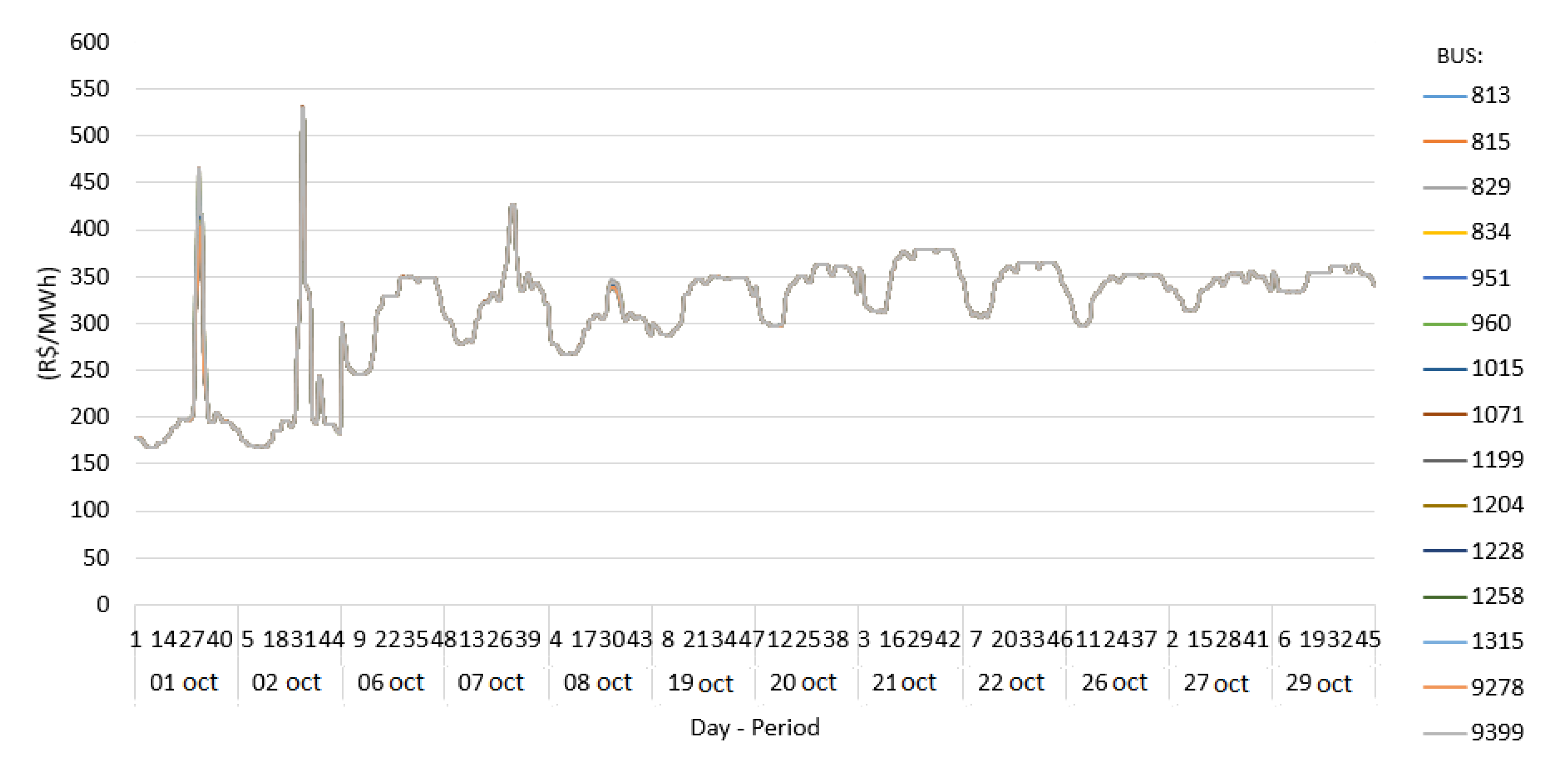
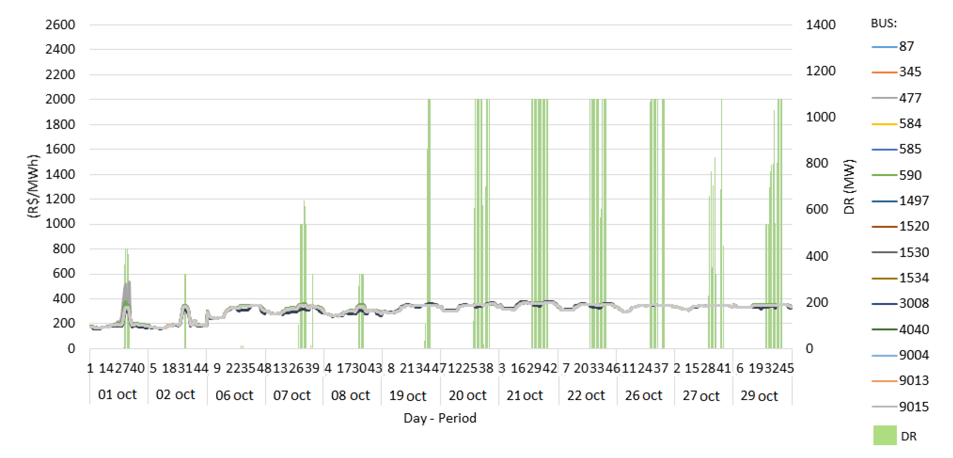
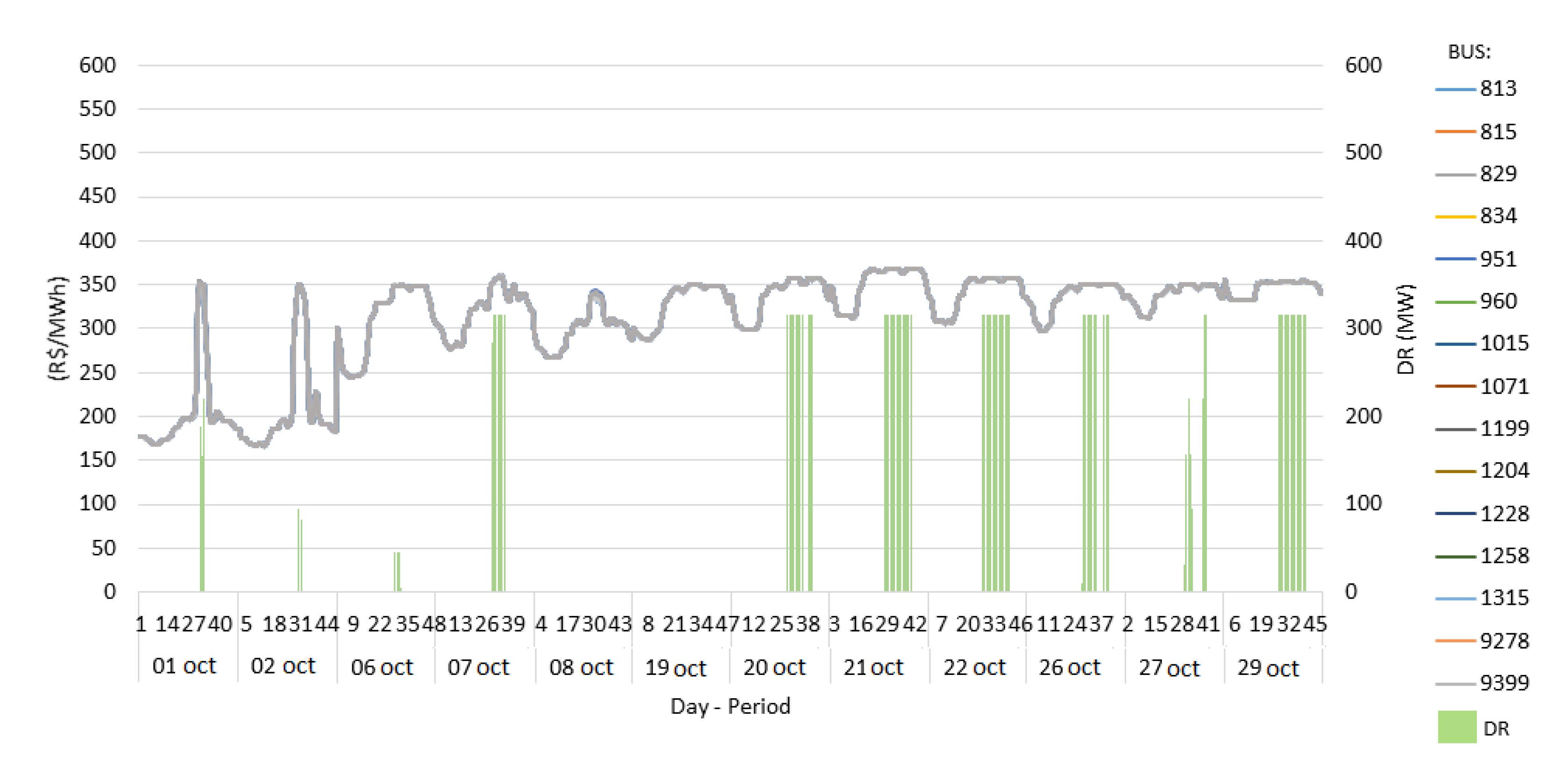
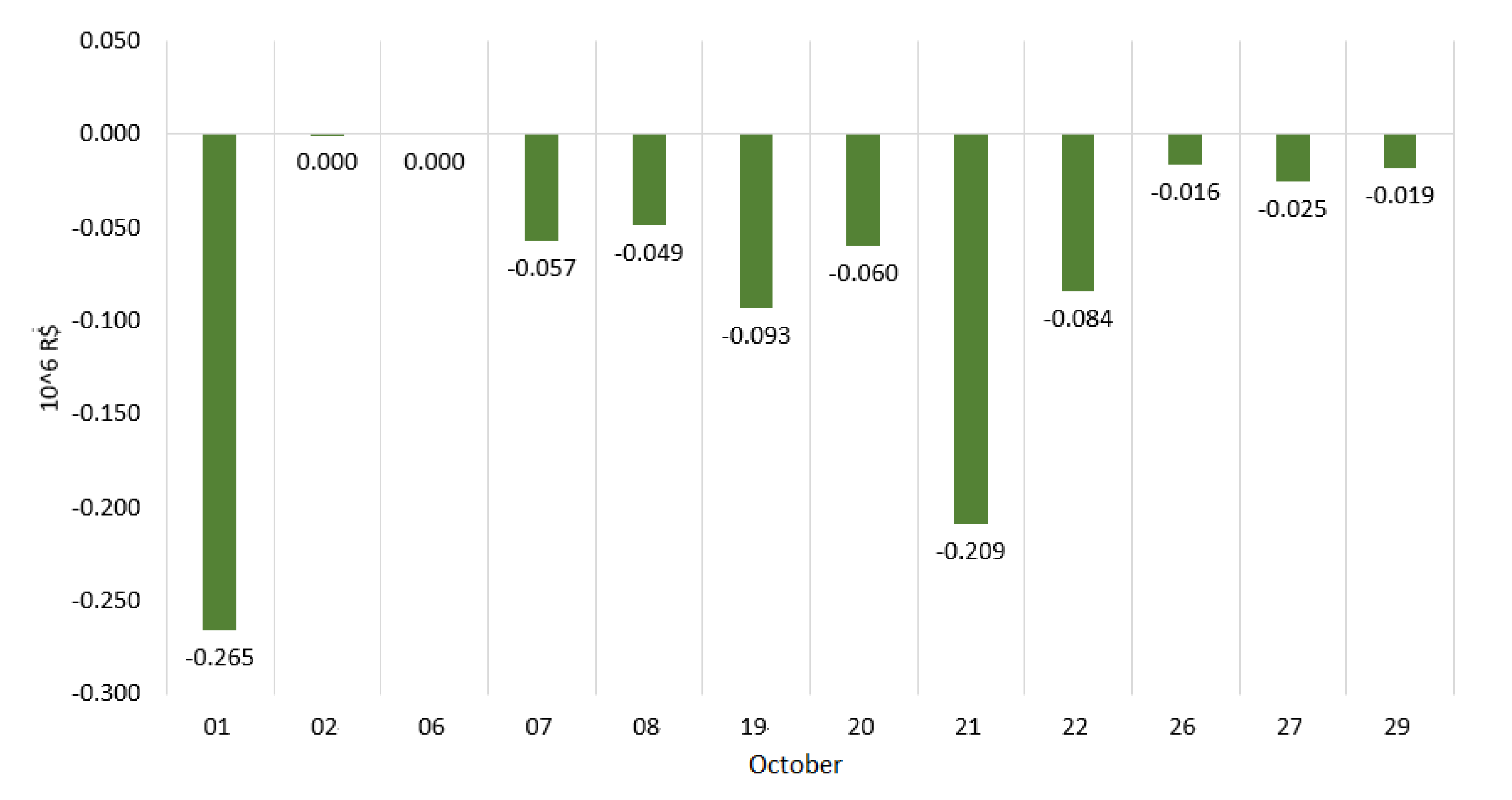
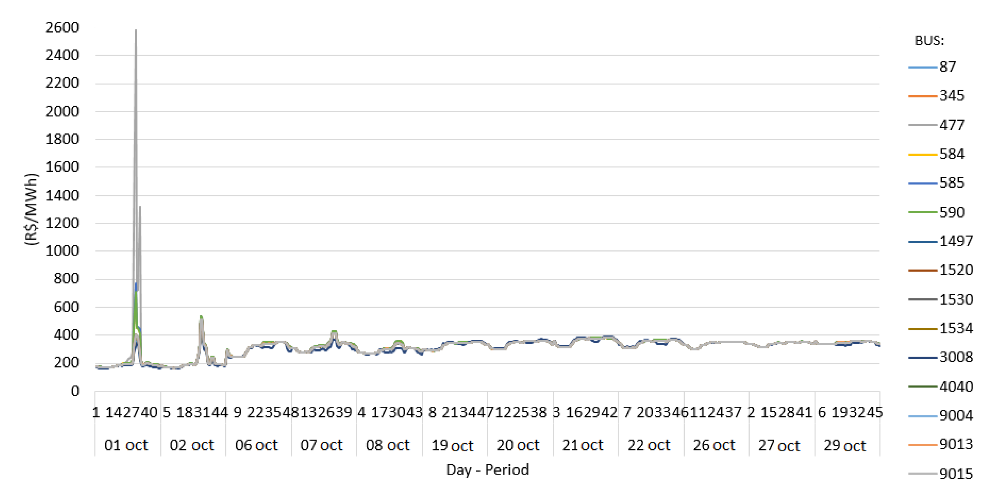
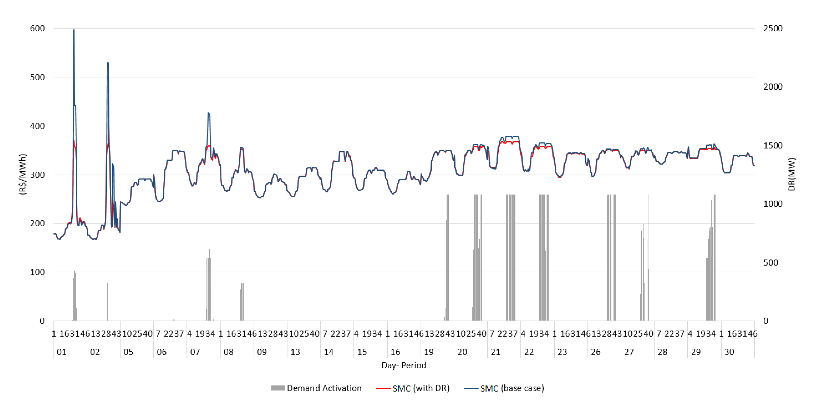
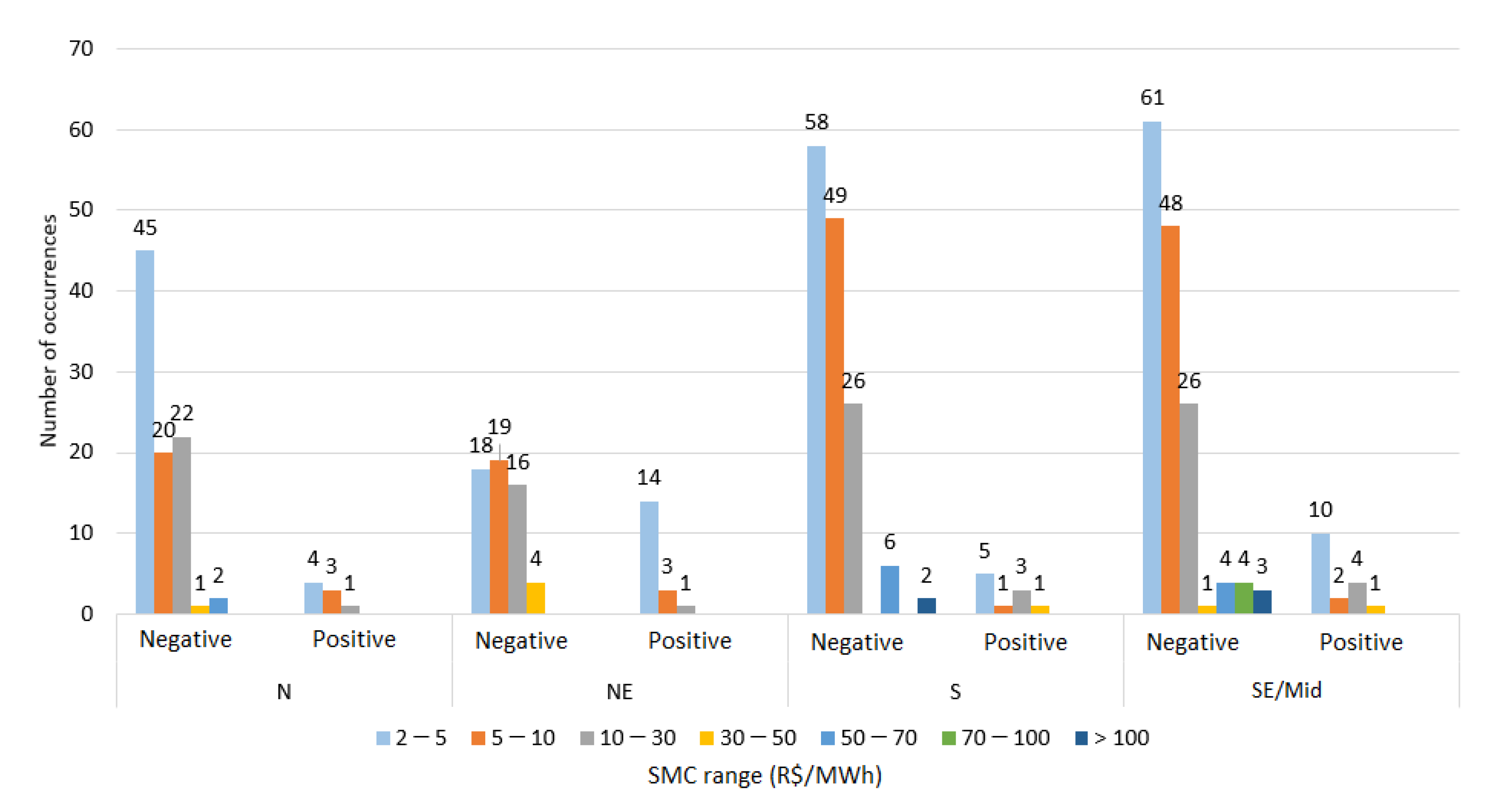
Based on the analysis results of marginal costs for each bus (BMC) and the average marginal cost for each subsystem (SMC) in which the system is divided, we concluded that the main benefit of the DR dispatch was to attenuate the peak values both for BMC and SMCs, which occurred at hours where the DR activation was allowed and whose energy requirements to meet demand proved to be more expensive. As a result, the DR dispatch allowed a reduction in the system operation cost by decreasing the load curve in peak demand hours.

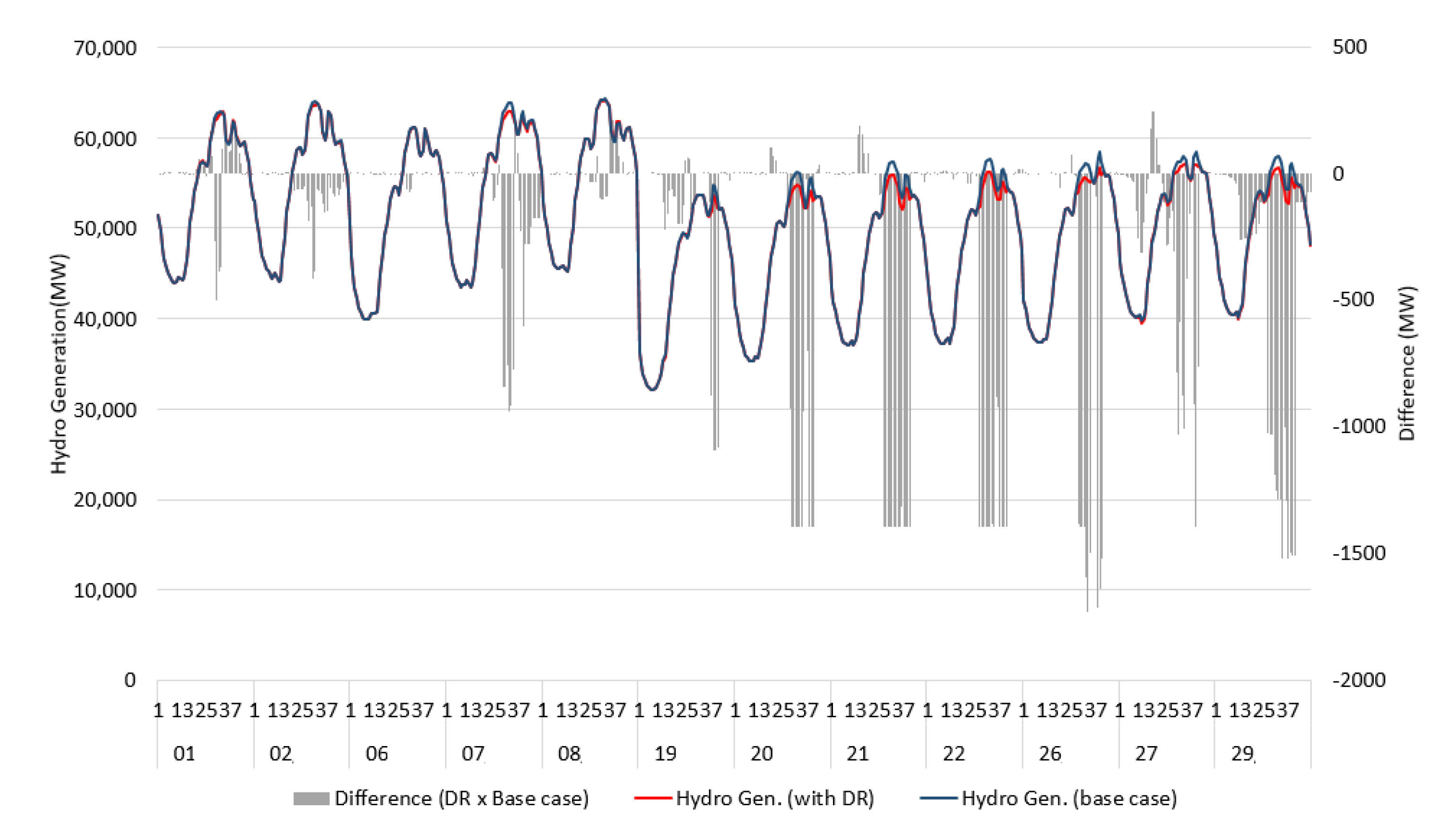
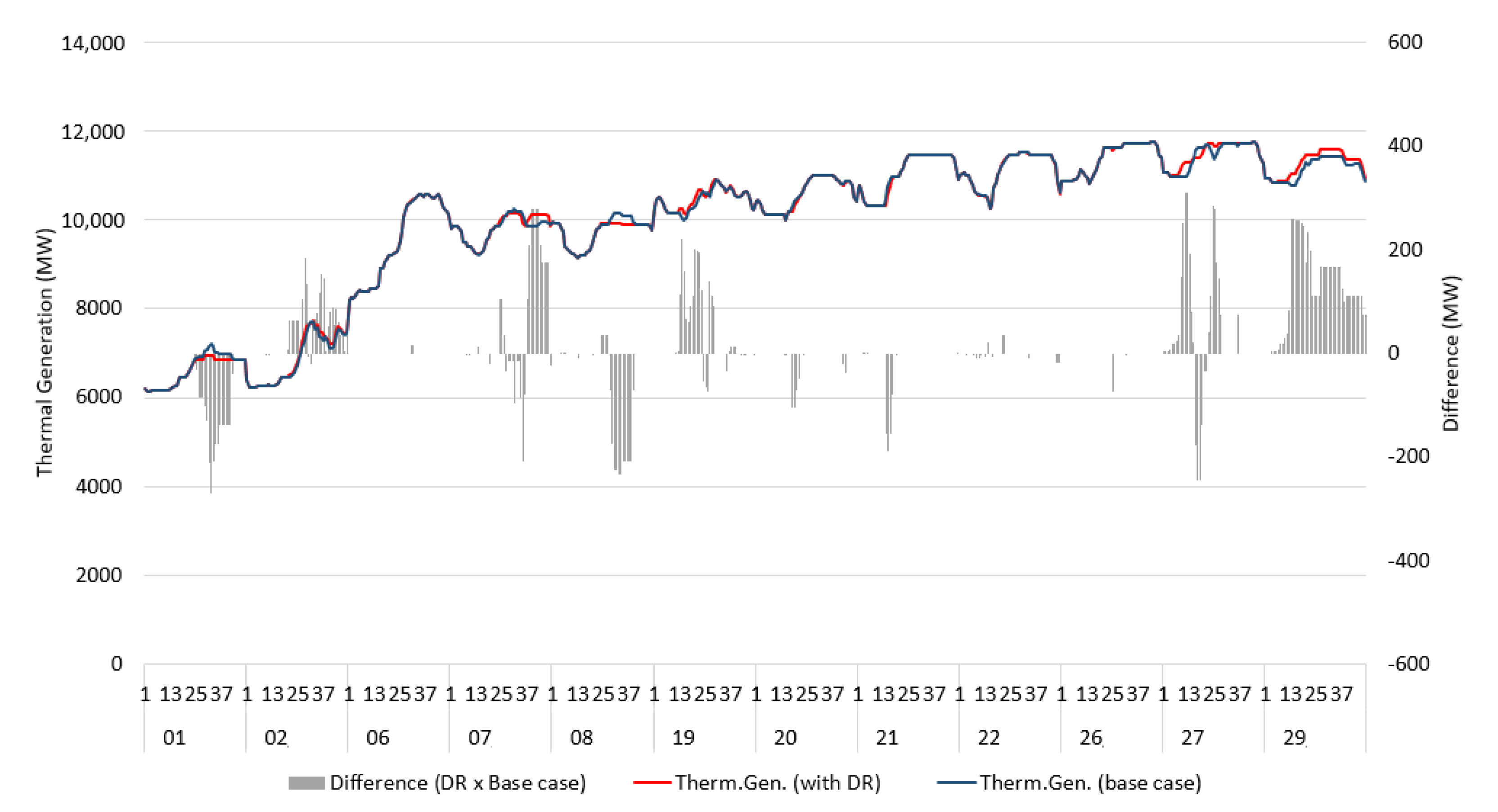
Moreover, with the application of DR there was a systematic reduction in hydro generation throughout the system, whereas the thermal dispatch varied from increasing in one region and decreasing in another one, depending on the case and system conditions. Finally, it was observed that the total operational cost of system was reduced, not only due to a decrease in present costs along the day but also by reducing the expected value of future costs, due to the higher storage in the reservoirs at the end of the day, yielded by the application of DR program.

As a final conclusion, we confirmed the feasibility of representing DR as a dispachable resource in the Brazilian system, with benefits in system operation cost and security of supply. The main limitation of this study is that we considered only the possibility of load reduction. For loads that are flexible in terms of the time window of application but cannot be curtailed, load shifting should be modeled, which was beyond the scope of the study. In this sense, in future works, we intend to assess the benefits/impacts of alternative/additional rules that may be considered for the DR program, such more rigid constraints for load reduction and the possibility of load shifting. In the work [14], modeling approaches for load shifting, either in a more flexible way or in fixed "load blocks" with the use of mixed integer linear programming techniques, are discussed and can be included in hydrothermal scheduling problems, such as the one considered in this study.

References

1. Blakers, A.; Stocks, M.; Lu, B.; Cheng, C. A review of pumped hydro energy storage. Prog. Energy 2021, 3, 022003. [Google Scholar] [CrossRef]
2. Dekka, A.; Ghaffari, R.; Venkatesh, B.; Wu, B. A survey on energy storage technologies in power systems. In Proceedings of the 2015 IEEE Electrical Power and Energy Conference (EPEC), London, ON, Canada, 26–28 October 2015; pp. 105–111. [Google Scholar] [CrossRef]
3. Wikramanayake, E.; Acharya, P.V.; Kapner, M.; Bahadur, V. Green hydrogen-based energy storage in Texas for decarbonization of the electric grid. In Proceedings of the 2021 IEEE Green Technologies Conference (GreenTech), Denver, CO, USA, 7–9 April 2021; pp. 409–415. [Google Scholar] [CrossRef]
4. Gellings, C.W. The concept of demand-side management for electric utilities. Proc. IEEE 1985, 73, 1468–1470. [Google Scholar] [CrossRef]
5. Zhang, Q.; Grossmann, I.E. Enterprise-wide optimization for industrial demand side management: Fundamentals, advances, and perspectives. Chem. Eng. Res. Des. 2016, 116, 114–131. [Google Scholar] [CrossRef] [Green Version]
6. Jabir, H.J.; Teh, J.; Ishak, D.; Abunima, H. Impacts of demand-side management on electrical power systems: A review. Energies 2018, 11, 1050. [Google Scholar] [CrossRef] [Green Version]
7. Jordehi, A.R. Optimisation of demand response in electric power systems, a review. Renew. Sustain. Energy Rev. 2019, 103, 308–319. [Google Scholar] [CrossRef]
8. U.S. Department of Energy (DOE). Benefits of Demand Response in Electricity Markets and Recommendations for Achieving Them; U.S. Department of Energy (DOE): Washington, DC, USA, 2006.
9. Behrangrad, M. A review of demand side management business models in the electricity market. Renew. Sustain. Energy Rev. 2015, 47, 270–283. [Google Scholar] [CrossRef]
10. FERC—Federal Energy Regulatory Commission. Demand Response and Advanced Metering 2019, Spring 200. Available online: https://www.ferc.gov/sites/default/files/2020-04/DR-AM-Report2019_2.pdf (accessed on 10 October 2021).
11. Smart Energy Demand Coalition—SEDC. Explicit Demand Response in Europe-Mapping the Markets 2017. Available online: https://smarten.eu/explicit-demand-response-in-europe-mapping-the-markets-2017/ (accessed on 12 October 2021).
12. Vahedipour-Dahraie, M.; Rashidizadeh-Kermani, H.; Najafi, H.R.; Anvari-Moghaddam, A.; Guerrero, J.M. Stochastic security and risk-constrained scheduling for an autonomous microgrid with demand response and renewable energy resources. Iet. Renew. Power Gener. 2017, 11, 1812–1821. [Google Scholar] [CrossRef]
13. Wang, S.; Bi, S.; Zhang, Y.J.A. Demand response management for profit maximizing energy loads in real-time electricity market. IEEE Trans. Power Syst. 2018, 33, 6387–6396. [Google Scholar] [CrossRef]
14. Luke, C.C.d.B.P.; de Freitas, D.; Maldonado, F.A.; Viola, L.; Bello, T.L.; Sagastizábal, C.; Luna, J.P.; Diniz, A.L.; Sabóia, C.H.; Cerqueira, L.F. Impact of Demand Response Programs in Unit-Commitment Problems in Energy Optimization 2021. Available online: https://www.cambridge.org/engage/miir/article-details/6114f74845805dcab985f079 (accessed on 20 February 2022).
15. Santos, T.; Diniz, A.; Saboia, C.; Cabral, R.; Cerqueira, L. Hourly pricing and day-ahead dispatch setting in Brazil: The dessem model. Electr. Power Syst. Res. 2020, 189, 106709. [Google Scholar] [CrossRef]
16. Basu, M. Optimal generation scheduling of hydrothermal system with demand side management considering uncertainty and outage of renewable energy sources. Renew. Energy 2020, 146, 530–542. [Google Scholar] [CrossRef]
17. Shen, J.J.; Shen, Q.Q.; Wang, S.; Lu, J.Y.; Meng, Q.X. Generation Scheduling of a Hydrothermal System Considering Multiple Provincial Peak-Shaving Demands. IEEE Access 2019, 7, 46225–46239. [Google Scholar] [CrossRef]
18. Bitaraf, H.; Rahman, S. Reducing Curtailed Wind Energy Through Energy Storage and Demand Response. IEEE Trans. Sustain. Energy 2018, 9, 228–236. [Google Scholar] [CrossRef]
19. Zhang, X.; Che, L.; Shahidehpour, M.; Alabdulwahab, A.; Abusorrah, A. Electricity-Natural Gas Operation Planning With Hourly Demand Response for Deployment of Flexible Ramp. IEEE Trans. Sustain. Energy 2016, 7, 996–1004. [Google Scholar] [CrossRef]
20. Cooke, D. Empowering Customer Choice in Electricity Markets 2011. Available online: https://www.iea.org/reports/empowering-customer-choice-in-electricity-markets (accessed on 20 September 2021).
21. Réseau de Transport d’Electricité-RTE. Bilan Électrique 2018. Available online: https://assets.rte-france.com/prod/public/2021-03/Bilan%20electrique%202018.pdf (accessed on 29 November 2021).
22. Torriti, J.; Hassan, M.G.; Leach, M. Demand response experience in Europe: Policies, programmes and implementation. Energy 2010, 35, 1575–1583. [Google Scholar] [CrossRef] [Green Version]
23. Martinez, V.J.; Rudnick, H. Design of Demand Response programs in emerging countries. In Proceedings of the 2012 IEEE International Conference on Power System Technology, POWERCON, Auckland, New Zealand, 30 October–2 November 2012. [Google Scholar]
24. Paterakis, N.G.; Erdinç, O.; Catalão, J.P. An overview of Demand Response: Key-elements and international experience. Renew. Sustain. Energy Rev. 2017, 69, 871–891. [Google Scholar] [CrossRef]
25. Hajibandeh, N.; Ehsan, M.; Soleymani, S.; Shafie-khah, M.; Catalão, J.P. The mutual impact of demand response programs and renewable energies: A survey. Energies 2017, 10, 1353. [Google Scholar] [CrossRef] [Green Version]
26. Diniz, A.L.; Souza, T.M. Short-term hydrothermal dispatch with river-level and routing constraints. IEEE Trans. Power Syst. 2014, 29, 2427–2435. [Google Scholar] [CrossRef]
27. Diniz, A.L.; Costa, F.D.S.; Maceira, M.E.; dos Santos, T.N.; Dos Santos, L.C.B.; Cabral, R.N. Short/mid-term hydrothermal dispatch and spot pricing for large-scale systems-the case of Brazil. In Proceedings of the 2018 Power Systems Computation Conference (PSCC), Dublin, Ireland, 11–15 June 2018; pp. 1–7. [Google Scholar]
28. Dos Santos, T.N.; Diniz, A.L. A dynamic piecewise linear model for DC transmission losses in optimal scheduling problems. IEEE Trans. Power Syst. 2010, 26, 508–519. [Google Scholar] [CrossRef]
29. Diniz, A.L.; Maceira, M.E.P. A four-dimensional model of hydro generation for the short-term hydrothermal dispatch problem considering head and spillage effects. IEEE Trans. Power Syst. 2008, 23, 1298–1308. [Google Scholar] [CrossRef]
30. Ottesen, S.Ø.; Tomasgard, A.; Fleten, S.E. Multi market bidding strategies for demand side flexibility aggregators in electricity markets. Energy 2018, 149, 120–134. [Google Scholar] [CrossRef]
31. Ponds, K.T.; Arefi, A.; Sayigh, A.; Ledwich, G. Aggregator of demand response for renewable integration and customer engagement: Strengths, weaknesses, opportunities, and threats. Energies 2018, 11, 2391. [Google Scholar] [CrossRef] [Green Version]
32. Burger, S.; Chaves-Ávila, J.P.; Batlle, C.; Pérez-Arriaga, I.J. A review of the value of aggregators in electricity systems. Renew. Sustain. Energy Rev. 2017, 77, 395–405. [Google Scholar] [CrossRef]
Figure 1. Classification of mainly DSM programs.
Energies 15 03928 g001
Figure 2. Price–quantity bid curves for demand response loads.
Energies 15 03928 g002
Figure 3. Southeast /Midwest BMC values on base case.
Energies 15 03928 g003
Figure 4. South BMC values on base case.
Energies 15 03928 g004
Figure 5. Southeast/Midwest BMC values and related buses with DR activation.
Energies 15 03928 g005
Figure 6. South BMC values and related buses with DR activation.
Energies 15 03928 g006
Figure 7. Southeast/Midwest SMC values.
Energies 15 03928 g007
Figure 8. Occurrences of SMC values—positive and negative differences.
Energies 15 03928 g008
Figure 9. Total system thermal generation.
Energies 15 03928 g009
Figure 10. Total system hydro generation.
Energies 15 03928 g010
Figure 11. Differences between total operational costs.
Energies 15 03928 g011