Article

A Flexible Deep Learning Method for Energy Forecasting

Research Center, Léonard de Vinci Pôle Universitaire, 92916 Paris La Défense, France
*
Authors to whom correspondence should be addressed.
These authors contributed equally to this work.
Energies 2022, 15(11), 3926; https://doi.org/10.3390/en15113926
Submission received: 15 April 2022 / Revised: 17 May 2022 / Accepted: 24 May 2022 / Published: 26 May 2022

Abstract

:
Load prediction with higher accuracy and less computing power has become an important problem in the smart grids domain in general and especially in demand-side management (DSM), as it can serve to minimize global warming and better integrate renewable energies. To this end, it is interesting to have a general prediction model which uses different standard machine learning models in order to be flexible enough to be used in different regions and/or countries and to give a prediction for multiple days or weeks with relatively good accuracy. Thus, we propose in this article a flexible hybrid machine learning model that can be used to make predictions of different ranges by using both standard neural networks and an automatic process of updating the weights of these models depending on their past errors. The model was tested on Mayotte Island and the mean absolute percentage error (MAPE) obtained was 1.71% for 30 min predictions, 3.5% for 24 h predictions, and 5.1% for one-week predictions.

1. Introduction

In December 2015, 196 countries agreed on an international treaty for limiting global climate change by reducing global warming. The main goal is to limit global warming to well below 2 °C by limiting the use of fossil fuels [1]. Due to both the availability and the cheap price of electricity in first world countries, and with the increase in the number of devices that need electricity to operate and the appearance of new ones such as electric cars, electrical grids and their growing effect on nature have become a significant concern.
Consequently, transition policies from fossils such as coal have been discussed in [2] while suggesting an increase in the use of renewable energies. In fact, the research in [3] predicts that the return of investment (ROI) for renewable energies is growing and will eventually become, in the future, similar to the ROI of fossils. This means that the economic expense that prevents governments from using renewable energies at large scales will eventually disappear with time. Indeed, this article is a part of the MAESHA project [4], which is funded by the European Union through the H2020 program. The goal of this project is the decarbonization of the future energy used in Mayotte and other islands by transforming the usual electrical grid into a smart grid that is able to manage the demand side to be adapted to the available generation at any time.
Moreover, different challenges arise when trying to manage the electrical grid of isolated areas because it is impossible to receive electricity from other countries or regions in the case of excessive demand, which can cause a blackout.
In addition, even though renewable energies are the main key to achieving the decarbonization of energy systems, their production varies significantly within short times due to environmental factors, such as the radiation of the sun or the speed of the wind, which can cause problems during peaks on the demand side.
Indeed, this brings the need for a smart grid that can detect, predict, and adapt to changes in order to match and manage the demand side with the availability on the supply side. As a consequence, predicting electrical load in advance is a very important challenge for demand-side management (DSM), especially in isolated areas [5].
Moreover, most of the current machine learning models are built to predict and are tested on the load demand of one region or country only, without taking into consideration the reusability of their models.
In fact, to predict the load of multiple islands with acceptable accuracy, it is important to build a flexible model in both space and time. First, as for the space, in order to predict the load in multiple regions without having to create different prediction models, it could be interesting to build a model combining standard machine learning models that are known to give good predictions with acceptable accuracy for the different situations or regions, thus having a reusable prediction model that can be used directly or with minimal changes on different regions, islands, countries, or even multiple buildings. The second challenge is how to simply build a flexible model that can predict in the range of multiple days or a week with an acceptable accuracy; at the same time, it should be able to predict a shorter range (the next 30 min or 24 h) with high accuracy.
Although some researchers have taken into consideration the testing of their models for multiple datasets, such as in [6], and other researchers have tried to build models that can predict for multiple months with relatively high accuracy [7], to our knowledge, none of the previous studies have taken into consideration the flexibility of their models in both space and time. The advantage of having generalized and reusable models is that they can, in general, save resources and time. More specifically, in cases such as the presented work in this article, the model can be simply applied to multiple regions (islands, cities, or whole countries).
For this reason, we propose in this paper a flexible hybrid model that relies on four neural network models to give a prediction, instead of relying on one single model. The advantage of this approach is that we already know some models can perform better for some regions and during some days or specific periods of time in general, while other algorithms can perform better in other regions and/or during other periods of time. Using a weights function that dynamically attributes weights to each algorithm depending on its previous error and accuracy, models that predict better in a specific period of time will, consequently, have a higher weight.
To validate the proposed model, it has been tested on two different datasets. The first dataset, provided by Electricity of Mayotte (EDM), consists of the previous loads registered from 2015 to 2020, with all-weather forecasts, and holiday data with a data granularity of 1 point every 30 min. The second dataset is “Panama Electricity Load Forecasting” from Kaggle. It has similar features with the exception of data granularity, which is 1 point per hour.
The paper is structured as follows: Section 2 presents the literature review about consumption forecasting/prediction. A brief description of Mayotte’s grid and the provided data is given in Section 3. Our approach is shown and detailed in Section 4. Experiments to validate our method are provided in Section 5. Conclusions and future perspectives are presented in Section 6.

2. Literature Review

Since energy demand is a set of ordered values representing an evolution of a quantity over time, it is handled as a time series forecasting problem.
Predicting energy consumption is frequently done in the short term: almost 60% of the studies employing data-driven models make hourly predictions [8]. It is equally interesting to see that the load in general is highly affected by cooling/heating (HVAC). Indeed, HVAC represents between 40% and 50% of the overall consumption of big buildings, such as offices, schools, or hotels [9]. Forecasting this consumption is often easier since the HVAC is fairly continuous over time and depends on external parameters such as local weather or time of the year [10].
Moreover, since load prediction is a time series forecasting problem, wavelet transform (WT) is an important tool to help find the different time and frequency features of the load curve [11]. Indeed, the use of WT in [12,13] was proven to be an important preprocessing step for the prediction. Ref. [14] has even proposed a framework of wavelet neural networks (WNN). Indeed, wavelet transform has been tried with different types of traditional and modern types of machine learning layers, such as feed-forward or convolutional layers [15].
On the other hand, it is not surprising to find familiar methods for time series, such as auto-regressive integrated moving average (ARIMA) [16,17,18], support vector machines (SVM) [19,20], and artificial neural networks (ANN), applied to this field, as shown in [21].
However, the review in [22] shows that artificial neural networks are the most efficient prediction models for load forecasting in the smart grids domain in general and for demand-side management specifically.
Indeed, ANNs are the most used methods in forecasting electrical load. They are widely employed in this field for their numerous advantages. In fact, the complexity of this task is considerable due to several factors/parameters, such as weather and holidays (linear and non-linear relationships), which is a well-suited problem for ANNs and their capacity to deal with non-linear relationships. ANNs are extremely robust and flexible, especially the multilayer perceptron (MLP); they do not need to be programmed but require data to train on. They are easy to implement but require some specialized knowledge to configure. They can be used alone [23], but they can also be combined with other models to obtain a hybrid prediction [16,18]. One of the disadvantages is the massive amount of data required to train the network. If there are not enough data to train the ANN, it will have difficulties generalizing and risk overfitting.
Another type of neural network widely used in the field of time series forecasting is the long short-term memory (LSTM). It is an artificial recurrent neural network architecture that can process entire sequences of data, making it a privileged model for handwriting recognition, speech recognition, and time-series data. It can be used alone [24,25] or with a convolutional layer for better results [26]. Some models combine neural networks with more classical models of time series forecasting. This combination aims to strengthen predictions and increase performance. This combination is designated as a hybrid model.

Hybrid Models

They represent combinations of two or more machine learning techniques. These models are more robust, as they have the advantages of the individual techniques involved and improve the forecasting accuracy. By combining separate models, complex structures can be modelled more accurately. More and more papers use a hybrid approach thanks to their performance [27,28,29]. They often combine linear with nonlinear models to be more robust and more accurate. The most traditional hybrid models are a combination of ARIMA for linear relationships and SVM or ANN to model the nonlinear component [17,18]. However, various methods and algorithms have been used in the prediction models, such as empirical mode decomposition (EMD), the extended Kalman filter (EKF), characteristic load decomposition (CLD), and the radial basis function neural network (RBFNN). Table 1 provides a brief review of these articles for load predictions covering short-term, mid-term, and long-term predictions and covering the various prediction algorithms used.
Although some of the previous research, such as [6], has been tested on multiple datasets from different countries, to our knowledge, none of them have been built to be general enough to be applied to any case, nor are they easily reusable without modifications to the code (especially isolated areas such as Mayotte where blackouts happen regularly because of high load consumption).
In addition, all previous articles have concentrated on having one prediction range (i.e., 1 h, 24 h, 1 week, etc.). However, having a prediction for 30 min can provide a higher accuracy than having a prediction for 1 week, and as a consequence, having multiple prediction ranges at the same time (very short-term prediction with very high accuracy and short- or mid-term prediction with slightly lower accuracy) can provide more stable results for the smart grid systems that have to interact and make decisions for one or more days in real-time.
Thus, in this paper, a generalized and reusable hybrid method is presented in Section 4. The proposed method is managed by an automatic process to optimize its hybrid parameters and to provide the best forecast at any time, in any region, and at multiple prediction ranges in the future.

3. Materials and Methods

One of the main problems of this work is how we can provide a generalizable load prediction model that can be applied to multiple regions, especially isolated ones (i.e., islands), such as Mayotte. In the following subsections, a detailed description of the general situation of the electrical grid on the island of Mayotte is given in Section 3.1, and a brief description of the proposed methods for different prediction ranges is given in Section 3.2.

3.1. Materials

Mayotte is a French tropical island. Its area is 374 km 2 , with 288,926 inhabitants; it has two thermal power plants and one biogas power plant. In addition, it has several photovoltaic generation plants built to achieve a transition from thermal generated energy to renewable energy. Table 2 shows the number of each type of generation source and the maximum power that can be generated with it, while Figure 1 shows the distribution of photovoltaic and thermal generators on Mayotte island.
As for the data provided by EDM, they consist of all historical data of the load and generation and all types of holiday data and weather forecasts that can be related to this prediction problem, as detailed in Table 3.

3.2. Methods

Although photovoltaic (PV) generation is not used in this article, it has been provided by EDM, as it will be used in future works on demand-side management, as the island regularly experiences short periods of blackouts due to the high demand or to its grid’s frequency issues. For this purpose, we propose in the current work a hybrid prediction algorithm that is basically built for 30 min predictions and that has also been adapted to be used to predict longer periods (24 h and 1 week) with relatively lower accuracy; all that is needed is minimal changes in the preprocessing phase. For instance, the real-time prediction (30 min later) uses all the preprocessing steps and earlier data available up to one month earlier. To predict the next 24 h, the proposed method is used without the wavelet transform part (only used for the previous day and earlier 7th, 14th, 21st, and 28th days), and to predict the next week, the wavelet transform and the first earlier day have been excluded. Figure 2 shows a flowchart detailing all differences and the steps taken for the different prediction ranges.
It is also important to mention that for all prediction ranges, the same hybrid model has been used without any modifications thanks to the standard machine learning models used (CNN, LSTM, CNN_LSTM, and MLP) and to the automatic weights update function.
A flowchart of the proposed hybrid model is given in Figure 3, and a detailed discussion of the suggested hybrid model with its automatic weights function, preprocessing, feature extraction, and selection is presented in Section 4.

4. Our Approach

In this paper, to forecast the electrical load in different regions such as Mayotte, we propose a hybrid prediction method. This method is composed of four deep learning models for time series analysis. Each model has its own characteristics and usefulness in different situations and periods of time. The combination of these four models will be able to handle any time series. To make the hybrid prediction, we decompose our approach into three steps:
A.
Preprocessing and feature selection to obtain the best results from the dataset;
B.
Hybrid model to combine four deep learning models for time series analysis;
C.
Weights function to optimize the forecast from the hybrid model.

4.1. Preprocessing and Feature Selection

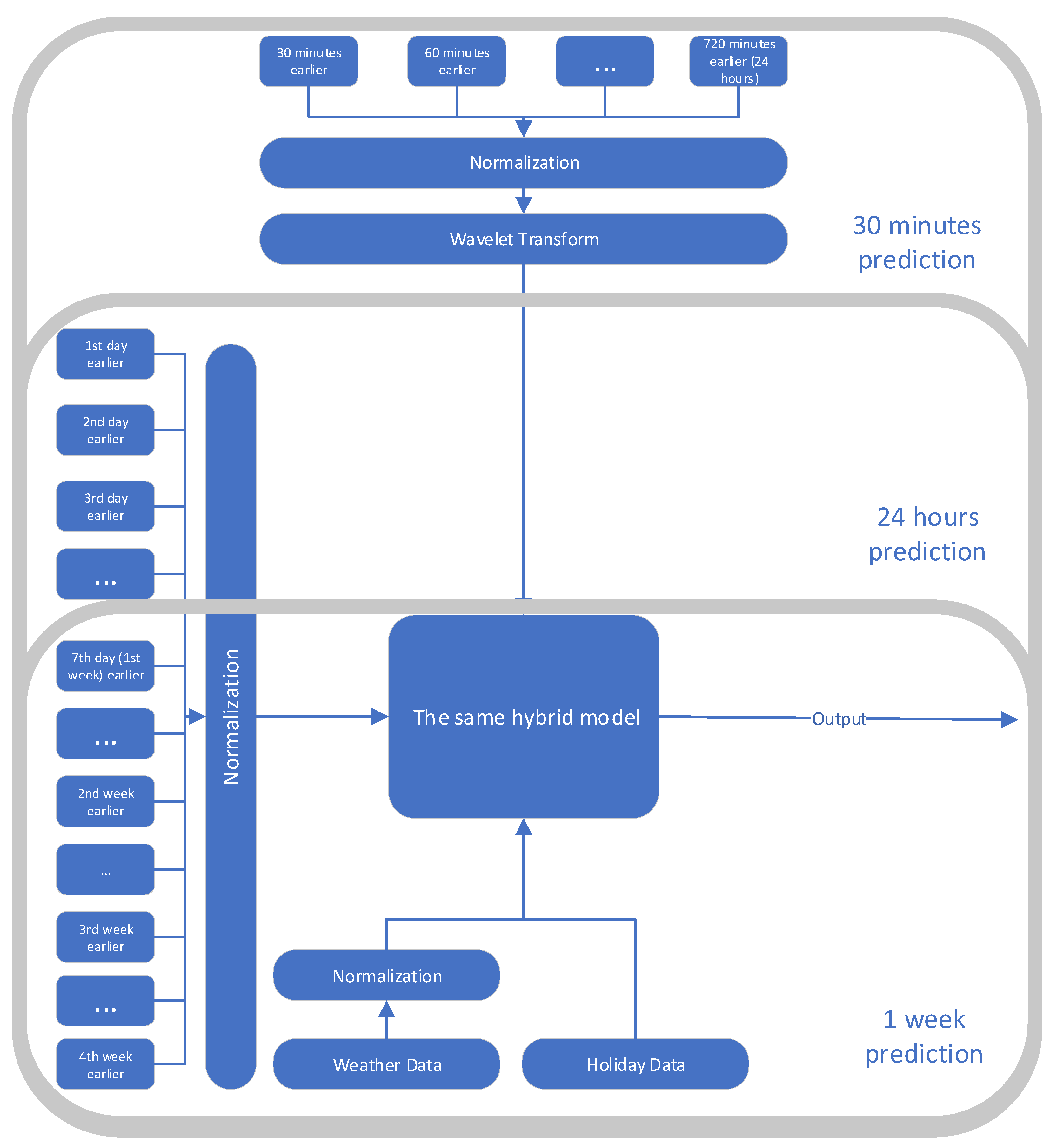
The objective of our model is to perform a short-term forecast and to make a prediction of up to 30 min, one day, and/or one week. The dataset consists of multiple columns, including the previous load data, the temperature (min, max, mean), the wind speed (min, max, mean), the global radiation, and more. We computed the correlation matrix of these columns to determine what features are most correlated with the data. The features selected were the previous load, the mean temperature, the public holidays, school holidays, and Ramadan days.

4.1.1. Interpolation

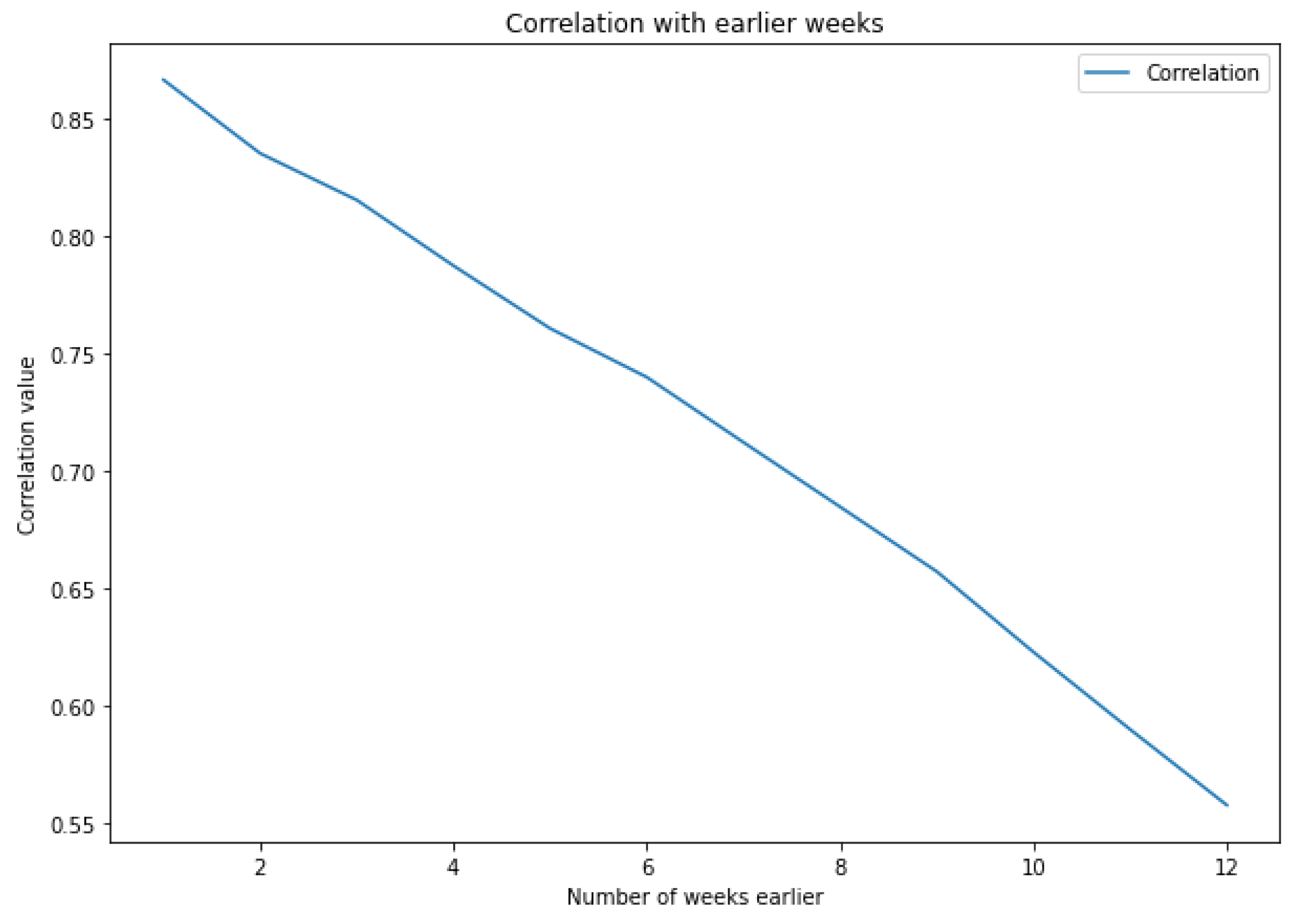
ML algorithms work better in time series that are relatively smooth. To minimize the large variations in the load curve, we tried to train the ML algorithms on both the original curve and the interpolated curve of the load. The prediction on the interpolated graph gave better results than the prediction on the original graph. While the interpolation is not directly used in our model, it was an important step because it helped in justifying and showing what kind of data are the more useful in order to obtain the best predictions. Indeed, following this logic of minimizing variations, we calculated the correlation with previous days and previous weeks to find the points that are the most similar to the point that we want to predict, and as a second step, we calculated the normalization which can minimize the margin of the curve without changing the general form of the curve.

4.1.2. Correlation and Seasonality

As for the previous load measurements, we noticed that all four models give better predictions when their input is relatively similar to the load that is being predicted. Thus, taking seasonality into consideration is an important factor in the prediction process [40].

4.1.3. Normalization

To evenly minimize the variations in the data, we wanted to smooth the general curve without changing its general form, so we used the Z-score normalization as defined in Formula (1):
Z = x μ σ ,
where x refers to the original curve; μ is the mean of x; σ is the standard deviation of x; and Z is the resulting curve after normalization. The normalization was implemented on each value separately and does not not affect the shape or the number of inputs.

4.1.4. Wavelet Transform

Wavelet transform is a time-frequency transformation that takes into consideration two parameters: scaling and shifting. Wavelet transform is generally used for denoising and compression. We use it here to obtain a compressed approximation of the last 24 h of the demand for electricity, in addition to the previously chosen data in Section 4.1.2. The advantage of using the approximated curve obtained by the wavelet transform is that it has a smaller size in the memory (compression) with less noise (denoising).
The wavelet transform W T ( a , b ) for a time series function S ( t ) is mathematically defined as in Formula (2):
W T ( a , b ) = 1 a S ( t ) . ψ ( t b a ) d t ,
where ψ (t) is the mother wavelet, a is the scaling parameter that deals with the frequency domain, and b is the shifting parameter that deals with the time domain.

4.2. Hybrid Model

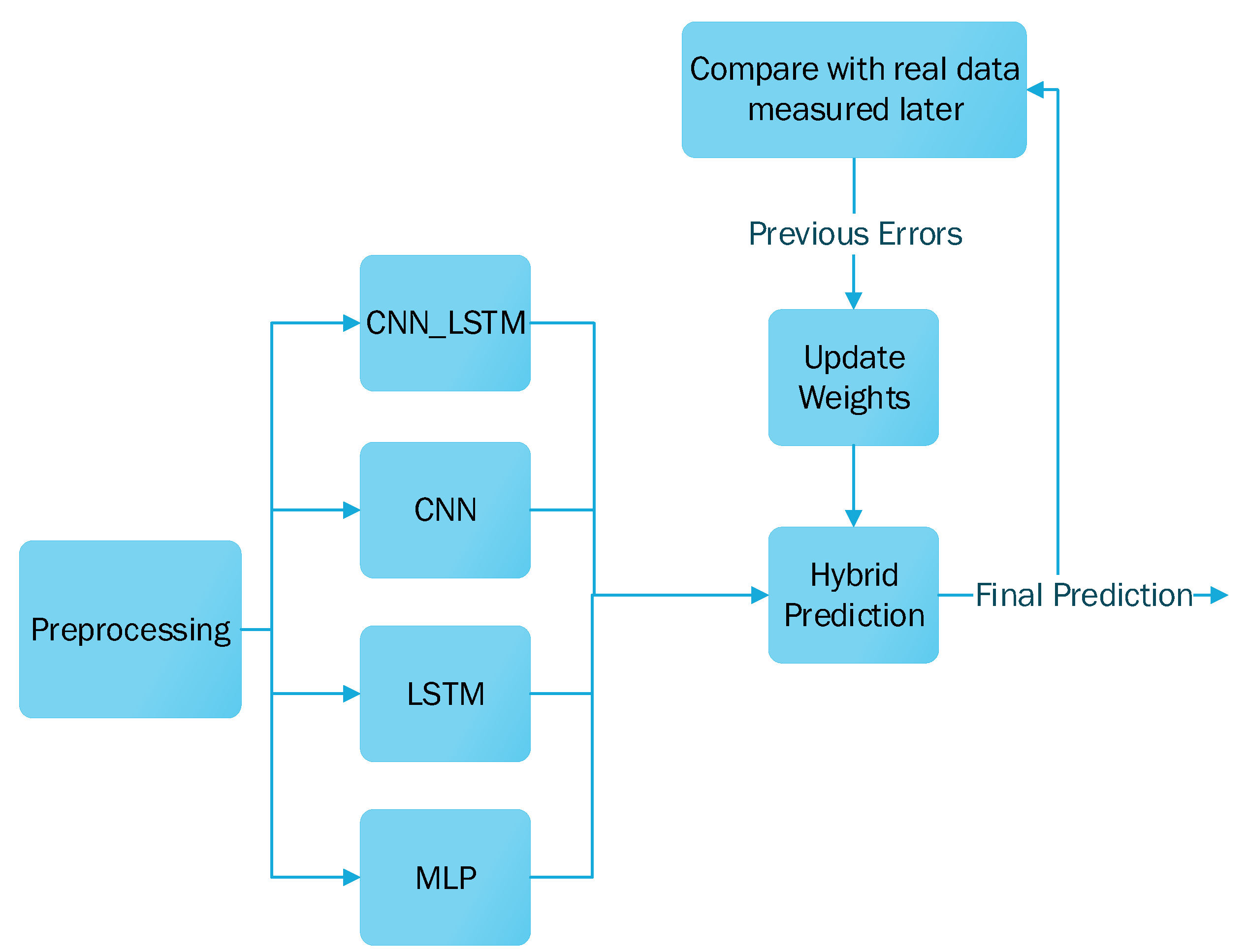
Our approach is based on a hybrid method that combines multiple deep learning models. Indeed, we used four deep learning models to have a generalizable and adaptive method for several time series or ranges of predictions. Our hybrid model is composed of multilayer perceptron (MLP), long short-term memory (LSTM), convolutional neural network (CNN), and CNN_LSTM, which is a combination of CNN and LSTM.

4.2.1. MultiLayer Perceptron (MLP)

MLP is a deep robust and reliable neural network and the most standard machine learning algorithm that can be used on most types of prediction problems.

4.2.2. Long-Short-Term-Memory (LSTM)

With LSTM layers, a special cell structure can order values of a given window to learn a sequence between them. The model learns a mapping from inputs to outputs and learns what context from the input sequence is useful for the mapping. In some cases, it should give better results compared to MLP since it captures and learns the sequence from a given window. Hence, it could be effective with the load’s curve showing sequences of marked steps. Very sensitive, it may become unstable with huge white noise.

4.2.3. Convolutional Neural Network (CNN)

CNNs are well-known for image processing and recognition, especially in computer vision. In our context, a conv1d layer synthesizes the time series, reduces the noise, and catches important seasoning. Its ability to learn and extract features from raw input may be useful for time series with complex relationships between input and output (previous values and future values).

4.2.4. CNN_LSTM

This consists of adding a conv1d layer before the LSTM cells. Overall, it seems to return better results than the others in many cases. It is used frequently in time series forecasting and is often considered to be one of the most precise models. The drawbacks are the need for a large amount of data to train it. Similar to classical CNN, it is better to train it with the original time series.
Some models will perform better on certain periods of time, while other models can outperform in other periods. The combination of models and how the most efficient models are preferred for a prediction are described in Section 4.3.

4.3. Weight Function

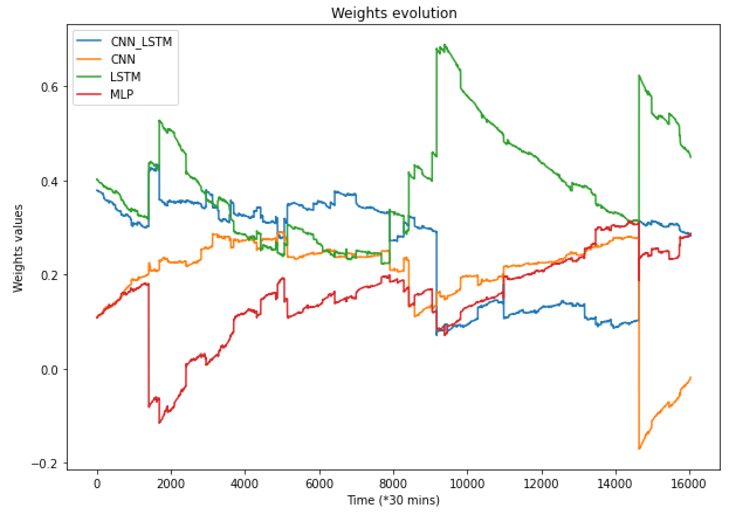
Since the loss of each model is different, a weight function aims to keep the best forecast for each prediction. Weight refers to a percentage. This percentage represents the importance attributed to a model for the final prediction. For a single model, its estimation will be multiplied by the weight related to this model. The final prediction is computed from the sum of all model predictions multiplied by their weights.
As the final prediction is calculated from the weights of each model, they all participate in the prediction of the final value with a greater or lesser weight depending on their previous results. Since the loss of each model is variable over time, the standard deviation is used to punish the models which would have too much dispersion in their predictions. Conversely, the more stable models with a constant error would be rewarded. Algorithm 1 explains the weights update process.
Algorithm 1: Weights calculation
    Input: Sequence of model errors values e r r o r s
    Output: Returns the updated weights n e w _ w e i g h t s
1:
l r ← 0.1
2:
models_last_values ← the last 30 model errors
3:
Sequence_values[] ← []
4:
Sequence_stds[] ← []
5:
for e r r o r in e r r o r s  do
6:
   value ← m a x ( e r r o r s ) e r r o r + m i n ( e r r o r s ) s u m ( e r r o r s )
7:
   add v a l u e in v a l u e s [ ]
8:
end for
9:
for l a s t _ v a l u e s in m o d e l s _ l a s t _ v a l u e s  do
10:
   std ← standardDeviation( l a s t _ v a l u e s )
11:
   add s t d in s t d s [ ]
12:
end for
13:
for s t d in s t d s  do
14:
   std ← m a x ( s t d s [ ] ) s t d + m i n ( s t d s [ ] ) s u m ( s t d s [ ] )
15:
end for
16:
new_weights ← o l d _ w e i g h t s + l r * v a l u e s * s t d s
17:
return new_weights
The weights are updated at each iteration, allowing us to keep constant control of the prediction and to ensure the best model will always have more importance compared to others. Thus, it is common to have a certain model with a high weight for a given period, and, for another, this model could have lower importance in the final prediction and therefore a lower weight due to its increasing errors.
Weights are updated at each new prediction more or less quickly depending on the learning rate. For a learning rate around 0.1 , there will be more variations in the importance of the models, whereas with a much smaller learning rate, such as 0.01 , the weights will take more time to update, and they will be more stable. The higher the learning rate is, the faster the weights update will be. The weights function is defined by an iterative equation:
n e w _ w e i g h t s o l d _ w e i g h t s + l r * v a l u e s * s t d s
where n e w _ w e i g h t s refers to a normalized array (a normalized value is inversely proportional to the value; the sum of all values is equal to one) of the weights of the function at the current prediction; o l d _ w e i g h t s refers to a normalized array of the weights at the previous prediction; l r refers to the learning rate; v a l u e s is a normalized array of the current error; and s t d s is a normalized array of the previous standard deviation during the last predictions.
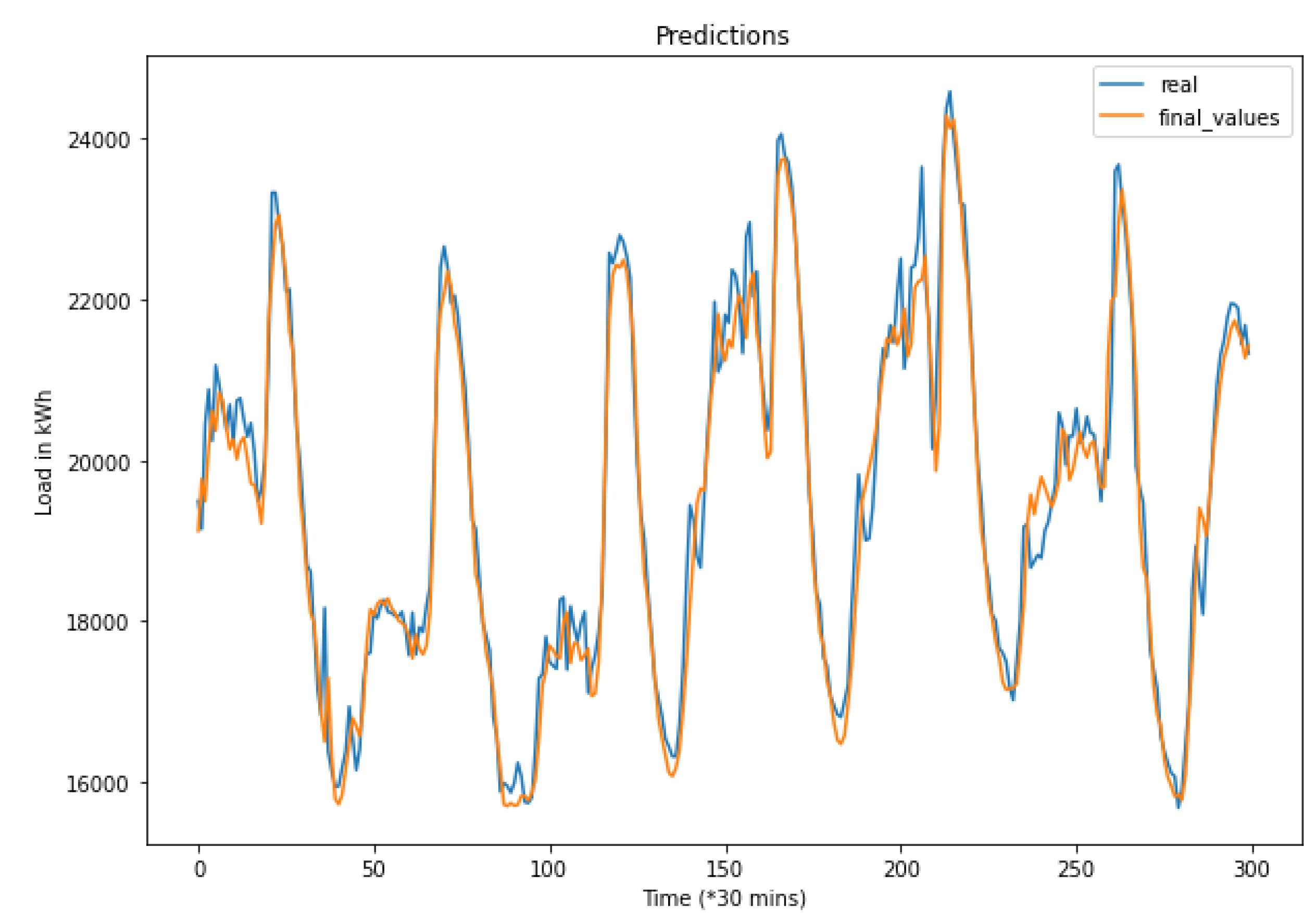
The final prediction is then obtained by summing each prediction algorithm result multiplied by its weight, as shown in the next equation:
f i n a l _ p r e d i c t i o n i = 1 4 w e i g h t i * p r e d i c t i o n _ v a l u e i ,
where i is the index of the corresponding algorithm.

5. Applications and Results

To test the efficiency and performance of the hybrid model, we tested our model on a dataset collected by the Electricity of Mayotte (EDM).

5.1. Mayotte Dataset

5.1.1. Preprocessing

For Mayotte island, we calculated the correlation between each day and the days in the week preceding it (Figure 4) and the correlation between each day and the same day in the previous weeks, up to 12 weeks (Figure 5).
The correlation with the previous days showed that the days are most correlated with their first, sixth, and seventh preceding day. However, the correlation with the sixth day is unimportant, as it is the first previous day for the seventh day, meaning it holds the same information.
Moreover, the correlation with the preceding weeks is a non-increasing line for the first 12 earlier weeks. Although it might be logical to think that the earlier weeks are simply correlated with each other, the training with multiple weeks has given better accuracy than by just taking only the first week earlier.
As a result, we took the loads the day before and the 4 weeks earlier as input for the prediction.

5.1.2. Hybrid Model

Since our method might be applied to multiple regions or countries other than Mayotte, and on different time ranges depending on the demand, the four deep learning models used must work on different time series and on multiple types of preprocessing. Their architecture (parameters, number of neurons, hidden layers, optimizer) is considered to be general enough and works over several time series without over-fitting. Their training parameters/layers that were used are described in Table 4. The loss used for the compilation is the mean absolute error (MAE).

5.1.3. Weight Function

After finishing the preprocessing phase, the data are then trained on 80 % of the time series data (which is equal to four years). The 20 % left (the year 2020) is used as a test set to experience a simulation of the weight function. The weight function combines the results of the four models for the hybrid prediction. Weights are attributed to each model representing their importance in the final prediction. Figure 6 shows the real test values versus the final predictions of the hybrid model on 300 measurements (9000 min), while Figure 7 shows how the weights are evolving over all the test data. It is worth mentioning that for algorithms having relatively large errors, their weights might decrease to reach negative values. While this does not have a mathematical meaning, it has proven to give better results in the hybrid predictions.
Table 5 regroups the mean absolute error (MAE) and the mean absolute percentage error (MAPE) computed on the whole test set for each model. For this case, the CNN and the LSTM showed the lowest errors, which correspond to the biggest weight assigned to this model in Figure 7. For the same test data, the MLP provides relatively bad results most of the time, which can be observed while checking the MAE, resulting in a small weight assigned to this model. However, given that the hybrid model is built to provide flexibility in all scales, it is important not to remove MLP, as it can prove to be more effective in different time ranges. Indeed, this idea has also been proven in Figure 7 at 14,000 (*30 min) when the MLP’s performance surpassed both CNN and LSTM.
The results show that our hybrid model follows the trend and seasonality of the time series, even for a 30-min forecast. The hybrid model is flexible and robust, and it is built to provide good forecasts for any time series.

5.2. Long-Term Predictions

Thanks to the standard machine learning algorithms that have been used, the proposed model can be applied to the load curves to predict different ranges. The only changes that were needed are in the preprocessing phase: by simply removing or adding the related preprocessing data, we can obtain a hybrid ML algorithm that can predict for 30 min, 24 h, or 7 days. Table 6 explains the different data used in the preprocessing phase for the different prediction ranges, while Table 7 shows the MAPE results for each prediction on the same test data.
Although the goal of this work is not to surpass all other algorithms but to provide a flexible model for prediction with acceptable accuracy, the proposed model has been compared with other known algorithms to show its efficiency for the case of day-ahead forecasting. Table 8 shows the results of these comparisons.

5.3. Panama Dataset

The proposed model has been tested on the Panama Dataset in order to validate the proposed model’s flexibility and reusability. The main requirement is that no changes should be applied to the models, their hyper-parameters, the preprocessing parameters, or the weights function. The hybrid model has been tested in different time ranges: 1 h (1 point per prediction), 24 h, and one week. The obtained results are shown in Table 9. It is worth mentioning that the prediction accuracy of the Panama Dataset is slightly lower, which is understandable as it has one measurement per hour, contrary to the Mayotte Dataset which has two measurements per hour. This proves the concept of Section 4.1.2 concerning the influence of the curve’s smoothness (or the variations in the curve) on the prediction accuracy.
It is worth mentioning that while this dataset has been tested by previous studies, such as [41], which tried to predict the monthly peak demand, and [42], which proposed a weekly prediction model, the goal of the proposed model in this article is not to outperform all previous models, but instead to propose a flexible model that can be reused to predict both load and generation with relatively good accuracy in the different temporal and spatial ranges.

6. Conclusions and Future Works

In this paper, we proposed a generalizable hybrid method using multiple standard deep learning models for electrical load short-term forecasting on the island of Mayotte. The results and applications show that the hybrid prediction is a generalizable method that can be used to predict different short-term ranges with only minor changes in the preprocessing phase and that can also be used to predict the load for different regions or countries without the need for any changes in the code.
Moreover, using all four models allows for obtaining more accurate results in a longer scale of time, as it minimizes the effects of changing seasons, holidays, and other events that might cause an increase in the prediction errors for some algorithms. Indeed, the weights assigned to each model and their continuous update maintain the best models for each time, and thus, this allows the proposed method to adapt according to the period of time that we are predicting. This weight system also brings stability and robustness to the prediction compared to stand-alone models.
In future work, this model can be applied to different regions, larger countries, or even continents such as Europe without being limited to special characteristics of some regions or cultures. This work is a first step for building a multi-agent smart grid that can predict and manage the electrical load using demand-side management (DSM), in accordance with the available renewable energies produced and where agents can choose the adequate prediction range while taking into consideration the accuracy of these predictions. The final goal is to decarbonize the production of electrical grids by relying on renewable energies only.

Author Contributions

Conceptualization, I.T. and G.G.; methodology, I.T., G.G., F.F. and N.N.; software, I.T. and G.G.; validation, G.G., F.F. and N.N.; resources, I.T., G.G., F.F. and N.N.; writing—original draft preparation, I.T. and G.G.; writing—review and editing, I.T., G.G., F.F. and N.N.; visualization, I.T.; supervision, G.G., F.F. and N.N. All authors have read and agreed to the published version of the manuscript.

Funding

This project has received funding from the European Union’s Horizon 2020 research and innovation programme under grant agreement No. 957843.

Institutional Review Board Statement

Not applicable.

Informed Consent Statement

Not applicable.

Data Availability Statement

Not applicable.

Conflicts of Interest

The authors declare no conflict of interest.

References

  1. The Paris Agreement|UNFCCC. 2021. Available online: https://unfccc.int/process-and-meetings/the-paris-agreement/the-paris-agreement (accessed on 7 February 2022).
  2. Spencer, T.; Berghmans, N.; Sartor, O. Coal transitions in China’s power sector: A plant-level assessment of stranded assets and retirement pathways. Coal Transit. 2017, 12/17, 21. [Google Scholar]
  3. Brockway, P.E.; Owen, A.; Brand-Correa, L.I.; Hardt, L. Estimation of global final-stage energy-return-on-investment for fossil fuels with comparison to renewable energy sources. Nat. Energy 2019, 4, 612–621. [Google Scholar] [CrossRef] [Green Version]
  4. The MAESHA Project. 2021. Available online: https://www.maesha.eu/the-project/ (accessed on 7 February 2022).
  5. Ramchurn, S.; Vytelingum, P.; Rogers, A.; Jennings, N. Putting the ’Smarts’ into the Smart Grid: A Grand Challenge for Artificial Intelligence. Commun. ACM—CACM 2012, 55, 86–97. [Google Scholar] [CrossRef] [Green Version]
  6. Haq, M.R.; Ni, Z. A New Hybrid Model for Short-Term Electricity Load Forecasting. IEEE Access 2019, 7, 125413–125423. [Google Scholar] [CrossRef]
  7. Lee, W.J.; Hong, J. A hybrid dynamic and fuzzy time series model for mid-term power load forecasting. Int. J. Electr. Power Energy Syst. 2015, 64, 1057–1062. [Google Scholar] [CrossRef]
  8. Amasyali, K.; El-Gohary, N.M. A review of data-driven building energy consumption prediction studies. Renew. Sustain. Energy Rev. 2018, 81, 1192–1205. [Google Scholar] [CrossRef]
  9. Pérez-Lombard, L.; Ortiz, J.; Pout, C. A review on buildings energy consumption information. Energy Build. 2008, 40, 394–398. [Google Scholar] [CrossRef]
  10. Liu, T.; Tan, Z.; Xu, C.; Chen, H.; Li, Z. Study on deep reinforcement learning techniques for building energy consumption forecasting. Energy Build. 2020, 208, 109675. [Google Scholar] [CrossRef]
  11. Rhif, M.; Ben Abbes, A.; Farah, I.R.; Martínez, B.; Sang, Y. Wavelet Transform Application for/in Non-Stationary Time-Series Analysis: A Review. Appl. Sci. 2019, 9, 1345. [Google Scholar] [CrossRef] [Green Version]
  12. Sun, W.; Ye, M. Short-Term Load Forecasting Based on Wavelet Transform and Least Squares Support Vector Machine Optimized by Fruit Fly Optimization Algorithm. J. Electr. Comput. Eng. 2015, 2015, 862185. [Google Scholar] [CrossRef] [Green Version]
  13. Bashir, Z.A.; El-Hawary, M.E. Applying Wavelets to Short-Term Load Forecasting Using PSO-Based Neural Networks. IEEE Trans. Power Syst. 2009, 24, 20–27. [Google Scholar] [CrossRef]
  14. Alexandridis, A.K.; Zapranis, A.D. Wavelet Neural Networks: A practical guide. Neural Netw. 2013, 42, 1–27. [Google Scholar] [CrossRef] [PubMed]
  15. Liu, J.; Li, P.; Tang, X.; Li, J.; Chen, J. Research on improved convolutional wavelet neural network. Sci. Rep. 2021, 11, 17941. [Google Scholar] [CrossRef]
  16. Zhang, G. Time series forecasting using a hybrid ARIMA and neural network model. Neurocomputing 2003, 50, 159–175. [Google Scholar] [CrossRef]
  17. Nie, H.; Liu, G.; Liu, X.; Wang, Y. Hybrid of ARIMA and SVMs for Short-Term Load Forecasting. Energy Procedia 2012, 16, 1455–1460. [Google Scholar] [CrossRef] [Green Version]
  18. Wang, X.; Meng, M. A Hybrid Neural Network and ARIMA Model for Energy Consumption Forcasting. J. Comput. 2012, 7, 1184–1190. [Google Scholar] [CrossRef]
  19. Dong, B.; Cao, C.; Lee, S.E. Applying support vector machines to predict building energy consumption in tropical region. Energy Build. 2005, 37, 545–553. [Google Scholar] [CrossRef]
  20. Ma, Z.; Ye, C.; Li, H.; Ma, W. Applying support vector machines to predict building energy consumption in China. Energy Procedia 2018, 152, 780–786. [Google Scholar] [CrossRef]
  21. Deb, C.; Zhang, F.; Yang, J.; Lee, S.E.; Shah, K.W. A review on time series forecasting techniques for building energy consumption. Renew. Sustain. Energy Rev. 2017, 74, 902–924. [Google Scholar] [CrossRef]
  22. Zhao, H.; Tang, Z. The review of demand side management and load forecasting in smart grid. In Proceedings of the 2016 12th World Congress on Intelligent Control and Automation (WCICA), Guilin, China, 12–15 June 2016; pp. 625–629. [Google Scholar] [CrossRef]
  23. Platon, R.; Dehkordi, V.R.; Martel, J. Hourly prediction of a building’s electricity consumption using case-based reasoning, artificial neural networks and principal component analysis. Energy Build. 2015, 92, 10–18. [Google Scholar] [CrossRef]
  24. Karevan, Z.; Suykens, J.A. Transductive LSTM for time-series prediction: An application to weather forecasting. Neural Netw. 2020, 125, 1–9. [Google Scholar] [CrossRef]
  25. Wang, J.Q.; Du, Y.; Wang, J. LSTM based long-term energy consumption prediction with periodicity. Energy 2020, 197, 117197. [Google Scholar] [CrossRef]
  26. Kim, T.Y.; Cho, S.B. Predicting residential energy consumption using CNN-LSTM neural networks. Energy 2019, 182, 72–81. [Google Scholar] [CrossRef]
  27. Ahmad, A.; Hassan, M.; Abdullah, M.; Rahman, H.; Hussin, F.; Abdullah, H.; Saidur, R. A review on applications of ANN and SVM for building electrical energy consumption forecasting. Renew. Sustain. Energy Rev. 2014, 33, 102–109. [Google Scholar] [CrossRef]
  28. Jallal, M.A.; González-Vidal, A.; Skarmeta, A.F.; Chabaa, S.; Zeroual, A. A hybrid neuro-fuzzy inference system-based algorithm for time series forecasting applied to energy consumption prediction. Appl. Energy 2020, 268, 114977. [Google Scholar] [CrossRef]
  29. Pao, H. Forecasting energy consumption in Taiwan using hybrid nonlinear models. Energy 2009, 34, 1438–1446. [Google Scholar] [CrossRef]
  30. Fan, S.; Chen, L. Short-term load forecasting based on an adaptive hybrid method. IEEE Trans. Power Syst. 2006, 21, 392–401. [Google Scholar] [CrossRef]
  31. Hooshmand, R.A.; Amooshahi, H.; Parastegari, M. A hybrid intelligent algorithm based short-term load forecasting approach. Int. J. Electr. Power Energy Syst. 2013, 45, 313–324. [Google Scholar] [CrossRef]
  32. Song, K.B.; Ha, S.K.; Park, J.W.; Kweon, D.J.; Kim, K.H. Hybrid load forecasting method with analysis of temperature sensitivities. IEEE Trans. Power Syst. 2006, 21, 869–876. [Google Scholar] [CrossRef]
  33. Liu, N.; Tang, Q.; Zhang, J.; Fan, W.; Liu, J. A hybrid forecasting model with parameter optimization for short-term load forecasting of micro-grids. Appl. Energy 2014, 129, 336–345. [Google Scholar] [CrossRef]
  34. Li, H.-z.; Guo, S.; Li, C.-j.; Sun, J.-q. A hybrid annual power load forecasting model based on generalized regression neural network with fruit fly optimization algorithm. Knowl.-Based Syst. 2013, 37, 378–387. [Google Scholar] [CrossRef]
  35. Ouyang, T.; He, Y.; Li, H.; Sun, Z.; Baek, S. Modeling and forecasting short-term power load with copula model and deep belief network. IEEE Trans. Emerg. Top. Comput. Intell. 2019, 3, 127–136. [Google Scholar] [CrossRef] [Green Version]
  36. Pallonetto, F.; Jin, C.; Mangina, E. Forecast electricity demand in commercial building with machine learning models to enable demand response programs. Energy AI 2022, 7, 100121. [Google Scholar] [CrossRef]
  37. Dudek, G.; Pełka, P.; Smyl, S. A hybrid residual dilated LSTM and exponential smoothing model for midterm electric load forecasting. IEEE Trans. Neural Netw. Learn. Syst. 2021, 1–13. [Google Scholar] [CrossRef] [PubMed]
  38. Hafeez, G.; Khan, I.; Jan, S.; Shah, I.A.; Khan, F.A.; Derhab, A. A novel hybrid load forecasting framework with intelligent feature engineering and optimization algorithm in smart grid. Appl. Energy 2021, 299, 117178. [Google Scholar] [CrossRef]
  39. Huang, Y.; Hasan, N.; Deng, C.; Bao, Y. Multivariate empirical mode decomposition based hybrid model for day-ahead peak load forecasting. Energy 2022, 239, 122245. [Google Scholar] [CrossRef]
  40. Xiao, L.; Shao, W.; Liang, T.; Wang, C. A combined model based on multiple seasonal patterns and modified firefly algorithm for electrical load forecasting. Appl. Energy 2016, 167, 135–153. [Google Scholar] [CrossRef]
  41. Ibrahim, B.; Rabelo, L. A Deep Learning Approach for Peak Load Forecasting: A Case Study on Panama. Energies 2021, 14, 3039. [Google Scholar] [CrossRef]
  42. Aguilar Madrid, E.; Antonio, N. Short-Term Electricity Load Forecasting with Machine Learning. Information 2021, 12, 50. [Google Scholar] [CrossRef]
Figure 1. Distribution of energy sources in Mayotte. Green represents the distribution of renewable energies (photovoltaic generation), and red represents the thermal stations. Source: EDM’s open data.
Energies 15 03926 g001
Figure 2. The different preprocessing steps used for each prediction range.
Energies 15 03926 g002
Figure 3. Hybrid prediction model.
Energies 15 03926 g003
Figure 4. Correlation between the day we want to predict and previous days in the week.
Energies 15 03926 g004
Figure 5. Correlation between the day to predict and the same days in previous weeks.
Energies 15 03926 g005
Figure 6. A sample of the real values vs predicted values for 30 min predictions. To avoid confusion, this is just a random slice of the test results (300 points) to better show the difference between the predicted and the real values.
Energies 15 03926 g006
Figure 7. The evolution of the weights on all the test data.
Energies 15 03926 g007
Table 1. The following table shows a sample of the various prediction methods used and how their proposed models do not have the flexibility to be reusable in both time and space variations.
ArticleTime Range FlexibilitySpatial FlexibilityComment
 [30]NoNoTested on historical energy load from New York Independent System Operator
[31]NoYesTested on Iran load dataset and New South Wales of Australian load dataset
[32]NoNoTwenty-four-hour load forecasting, tested on one dataset
[33]NoYesTested on four different microgrids
[7]NoNoTheir model is applied separately to the household, public, service, and industrial sectors
[34]NoNoTheir proposed model has only yearly prediction
[35]YesNoDay ahead and week ahead forecasting
[36]YesNoOne hour-ahead, peak day-ahead, and valley day-ahead forecasting
[37]NoYesTested on multiple European countries
[38]NoYesTested on 5 states in Australia
[39]NoYesTested on New South Wales (NSW) and Victoria (VIC) in Australia
Table 2. The different types of power generators, their counts, and their maximum generation.
Type of GenerationCountPower Capacity (KW)
Thermal272,900
Biogas11067
Photovoltaic (PV)9517,229
Table 3. Details about the data provided by EDM.
DataRangeGranularity
Load (demand)2016–202030 min
PV generation2016–202030 min
Public holidays2016–2025day
School holidays2016–2021day
Ramadan2016–2025day
Weather predictions2016–20201 h
Table 4. Models parameters & architecture..
ModelsArchitectureEpochsOptimizer
CNN_LSTM1 × Conv1D17Adam
2 × LSTM
2 × Dense
Output
CNN1 × Conv1D25Adam
1 × Flatten
2 × Dense
Output
LSTM2 × LSTM30Adam
1 × Dense l r = 0.003
Output
MLP1 × Flatten50Adam
2 × Dense
Output
Table 5. Validation of the hybrid model (MAE and MAPE).
ModelMAE (kWh)MAPE (%)
CNN_LSTM421.501.92
CNN343.671.61
LSTM343.491.61
MLP451.772.06
Hybrid Model372.081.71
Table 6. Data used in the preprocessing phase for the different prediction ranges.
Prediction Range30 min24 h7 Days
Waveletsyesnono
24 h earlieryesyesno
4 weeks earlieryesyesyes
Table 7. The resulting MAPE for each prediction range.
Prediction Range30 min24 h7 Days
MAPE (%)1.713.55.1
Table 8. A comparison with other known models for day-ahead forecasting (24 h prediction).
ML AlgorithmMAPE (%)
LightGBM3.6
XGBoost3.72
Random Forest3.9
CatBoost3.74
Hybrid Model3.5
Table 9. The resulting MAPE for each prediction range (Panama Dataset).
Prediction Range60 min24 h7 Days
MAPE (%)1.884.695.31
Publisher’s Note: MDPI stays neutral with regard to jurisdictional claims in published maps and institutional affiliations.

