A Two-Stage EV Charging Planning and Network Reconfiguration Methodology towards Power Loss Minimization in Low and Medium Voltage Distribution Networks

Abstract

The topic of power loss reduction in distribution systems has gained significant attention over recent years. Despite the efforts of the European Union towards the minimization of power losses, the decarbonization of the transport sector has raised several concerns, since charging overlaps of Electric Vehicles (EVs) can cause extensive power losses and power quality issues. Considering these, the present paper proposes a two-stage EV charging planning and Network Reconfiguration (NR) methodology, addressing the problem of power loss minimization in both Low-Voltage (LV) and Medium-Voltage (MV) Distribution Networks (DNs), respectively. In the first stage, considering the key role of the aggregator, the EV charging planning is applied to LV DN. In the second stage, the NR technique is applied to the MV DN, by taking into account the hourly power demand of LV DNs as obtained by the aggregators. The proposed methodology has been applied on a benchmarked MV network for which each node is represented by a real LV network. The results indicate that the proposed methodology could yield up to a 63.64% power loss reduction, in respect to the base scenario, i.e., no charging planning and no NR are applied.

1. Introduction

The issue of power losses has gained significant attention over recent years. The European Union (EU) has recently proposed the recast COM/2021/558 [1] of the Energy Efficiency Directive 2012/27/EU [2], in which Article 25 provides the guidelines for member states’ energy authorities to include the assessment of power losses as a separate section in their annual progress achieved in energy efficiency improvements. The recast highlights the necessity of power loss reduction, since they constitute a significant amount of the annual produced energy at distribution level, as presented by the Council of European Energy Regulators (CEER) [3]. Specifically, according to the report [3], the annual distribution power losses of the member states are presented separately, and the conclusions insist on the need for a power loss decrement in order to improve the efficiency of the systems. The issue of power losses from the perspective of the Distribution Network’s (DNs) efficiency is also addressed in a technical report [4], which indicates that the Distribution System Operators (DSOs) should be encouraged to reduce the distribution losses, since they are the key actors to ensure the efficient operation of the system.

Apart from the efficiency of the distribution systems, the power losses directly affect the energy price. The EU Agency for the Cooperation of Energy Regulators (ACER) published a report referring to the methodologies of distribution tariff methodologies [5]. According to the report, the cost of the power losses is either transferred directly onto the final consumers as distribution tariffs or is included in the bid price in the energy markets. Either way, the consumers are charged for the systems’ losses.

Despite the effort of the EU to minimize the losses of the systems, the power grids are facing new challenges. The environmental crisis has triggered several changes towards the reduction of greenhouse gas emissions (CO₂). At the end of 2019, the European Commission announced the European Green Deal, which is a set of policies aiming to transform the EU into the first climate neutral continent [6]. The main aim of the European Green Deal is the 55% reduction of greenhouse gas emissions by 2030 and the 100% reduction by 2050. In order to meet these objectives, in July 2021, the European Commission presented a set of proposals, including the decarbonization of the transport sector. Based on this, the member states should provide appealing incentives and recommendations to the consumers in order to replace their conventional cars with hydrogen Fuel Cell Vehicles (FCVs) [7] or Electric Vehicles (EVs), i.e., Plugged-in Hybrid EVs (PHEVs) [8] or Battery EVs (BEVs) [9]. Apart from FCVs, the uncertainties of EVs, i.e., time of arrival and State-of-Charge (SoC), in combination with their uncontrolled charging can increase the peak demand of energy consumption and consequently can lead to extensive power losses [10]. Thus, it is essential to employ methods in order to alleviate the negative impacts of EVs’ integration into DNs [11].

Considering the aforementioned issues, two well-established techniques towards the minimization of power losses are Network Reconfiguration (NR) [12] and the optimal charging of EVs [13]. These two techniques refer to different voltage levels and in many studies are mainly employed separately. On the one hand, NR is applied to Medium-Voltage (MV) systems in order to determine the optimal topology of DN in terms of power loss minimization [14]. Even though in studies [15,16,17,18] the integration of EVs was also considered, their charging plan was not studied. Instead, the EVs were utilized to examine the hosting capacity of the system [15] or only to formulate the daily load curve [16,17,18]. Despite previous studies, a different approach was presented in [19]. Specifically, in [19], the authors focused on the optimal size and location of EV charging stations under NR, considering the impact of charging stations into the DN [20]. On the other hand, the smart charging of EVs is used for Low-Voltage (LV) DNs and deals with power losses, voltage violation and transformer overloading issues, due to the high penetration and uncontrolled charging of EVs [21]. The problem of optimal EV charging has been addressed from different perspectives, such as power loss minimization and improvement of voltage profile [13], peak demand reduction [22] and decrement of greenhouse gas emission [23].

Some authors have also developed methodologies in order to combine both NR and optimal EV charging scheduling. Several studies have been conducted considering two optimization stages, meaning that NR and optimal EV charging are subjected to different objective functions. For instance, the authors in [24] deployed NR in order to minimize power loss, voltage deviation and load balancing indexes, while the smart charging scheduling was applied to improve peak-valley filling. A similar approach was also presented in [25], in which instead of load balancing, the voltage stability index was included. A two-stage optimization methodology was also presented in [26], where the objective to be minimized in MV DN was the cost of power, losses and switching, while in LV DN it was the charging cost. The combination of NR alongside with EV’s coordinated charging under the same objective function has also been examined. Despite the aforementioned studies, the combination of NR alongside with EV’s coordinated charging under the same objective function has also been examined. The researchers in [27] proposed a methodology considering the minimization of power losses and the power cost. A similar approach was presented in [28], in which the authors developed a methodology in order to minimize the total power cost of the system.

In the aforementioned studies, the smart charging of EVs is assumed to be implemented in charging stations. A different perspective was presented in [29], where the proposed methodology was implemented considering residential chargers. The main objective of the charging plan was cost minimization along with the peak-valley filling. The authors in [30] also considered that EVs will be charged in residential infrastructure. Still, the minimization of power losses referred only to MV DN. In both studies, the authors did not take into account the topology of LV DN.

A brief description of the implemented methodologies so far is presented in

Table 1. Literature review of the methodologies NR and optimal charging scheduling.

Reference	Objective Function at MV DN	Objective Function at LV DN	Multi-Hour Analysis	Optimization Stages	Residential Chargers	Consideration of VL DN Topology
Ref [24]	Power Loss index Load balancing index Voltage deviation index	Peak-Valley filling	✓	Two stages	✕	✕
Ref [25]	Power loss index Voltage deviation index Voltage stability margin index	Peak-valley price	✓	Two stages	✕	✕
Ref [26]	Cost of power Cost of network losses Cost of switching	Charging cost	✓	Two stages	✕	✕
Ref [27]	Cost of power losses Cost of power		✓	One stage	✕	✕
Ref [28]	Cost of buying active and reactive power Switching cost Cost of power losses Cost of selling active and reactive power		✓	One stage	✕	✕
Ref [29]	Power losses	Valley-Filling Charging cost	✓	Two stages	✓	✕
Ref [30]	Power losses	Power losses	✓	Two stages	✓	✕
Present study	Power losses	Power losses	✓	Two stages	✓	✓

. From the literature, it has been identified that the majority of the proposed methodologies examine the impact of EV charging scheduling at the MV level. Yet, the existing studies are based on the assumption that EVs will be plugged in charging stations or charging lots. The residential charging infrastructure is omitted, even if in some countries the installation of charging slots in blocks of flats is obligatory [31]. Although in studies [29,30] the authors included residential chargers, the charging scheduling is implemented by assuming that EVs are connected to charging stations or charging lots. Consequently, the topology of LV DNs is not of concern, since all EVs are plugged in at a single charging point. Considering the aforementioned, the novelty of the present paper lies in the fact that it considers the topology of LV DN and examines the impacts of smart charging scheduling at the LV level.

Based on this and taking into account the efforts of the EU towards power loss minimization, in this study a two-stage optimization scheme is proposed, including NR and EV smart scheduling. In the first stage, a day-ahead smart charging plan is proposed at LV DN, considering the technical constraints of DNs [2] as well as the key role of aggregators in DNs’ operation [32]. More specifically, the aggregator, which is responsible for the LV DN, applies the smart EV charging schedule to a real LV DN of 109 nodes in order to minimize the power losses of the network. The proposed methodology is a distributed one. Considering that at each node of the MV DN a LV DN is connected, the EV charging scheduling is applied at each LV DN individually. A similar approach, in terms of distributed control algorithms, is presented in papers [33,34,35], where the authors employed distributed algorithms in order to minimize the total energy cost of the EVs’ fleet. In the second stage, the DSO applies the NR to determine the next day’s optimal topology of the MV DN, considering the load curve formulated after the deployment of the charging plan at the LV DNs. This can lead to further reduction of power losses at the MV DN. In both stages, the Unified Particle Swarm Optimization (UPSO) metaheuristic algorithm is employed, considering the complexity of the problem.

Therefore, the main contributions of the present study can be summarized as follows:

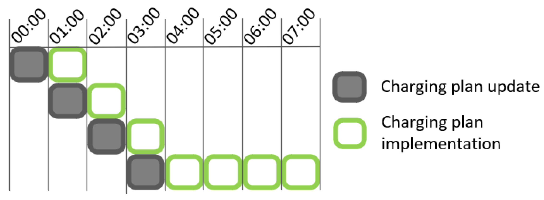
• Real-time hourly EV smart charging scheduling update in LV DNs that deals with uncertainties in EVs’ time of arrival due to forecasting errors.
• Consideration of residential EV charging by taking into account the layout of a real LV DN and using real data about the loading of the network and its electrical characteristics, i.e., lines’ length and impedance.
• Power loss minimization in LV DNs due to the proper time allocation of EVs’ charging that in turn results in smoother loading for the nodes of the MV DN and in lower power losses at the MV network.
• Further power loss reduction by planning the NR application on the MV DN for the next day. The optimal reconfigured topology for the MV DN is constant for the whole day in order to avoid frequent switching operations, e.g., hourly NR, that could result in frequent disturbances and could impose the need for the frequent replacement of the switches.
• Simple and straightforward cooperation between the DSO and potential aggregators in order to minimize the power losses and improve the power quality and the efficiency in both MV DN and LV DNs.

The rest of the paper is organized as follows. Section 2 presents the mathematical formulation of the objective function as well as the description of the proposed smart charging algorithm and the NR. In Section 3, the analysis of UPSO for both charging scheduling algorithm and NR is presented. Section 4 includes the description of the examined LV DN and MV DN. Additionally, in Section 4, the results of the study are presented and discussed. Finally, Section 5 concludes the paper.

2. Problem Formulation

2.1. Objective Function

The proposed methodology addresses the problem of power loss minimization in both MV and LV DNs. The optimization is executed at two stages. In the first stage, the aggregator which is responsible for each LV DN defines the day-ahead charging of EVs at a residential charging infrastructure, by applying the proposed charging scheduling technique. Considering the resistance of the LV distribution lines, the main aim is to minimize the power losses of LV DN by preventing the extensive power demand overlaps. In this way, lines’ overloading due to uncoordinated charging can be prevented, and the current of the lines can be alleviated. In the second stage, the DSO determines the day-ahead optimal topology of the system, by applying the NR. For the execution of NR, the hourly day-ahead load demand at each MV node is obtained from the total hourly load demand of the LV network that is coupled to each MV node. In both stages, the objective to be minimized is the power loss, referring to either LV or MV DN, and is expressed as follows:

$$\mathrm{OF}=\min {\displaystyle \sum _{t=1}^T{\displaystyle \sum _{\begin{array}{l}i,j=1\\ i\ne j\end{array}}^n{g}_{i,j}\left(V_i^2-V_j^2-2V_i{V}_j\cos \left({\theta }_i-{\theta }_j\right)\right)}}$$

(1)

where:

t indicates the hour when the objective function is applied; T denotes the total number of hours for which the analysis is conducted; i, j are indexes referring to the buses of the system; $g_{i,j}$ is the conductance between nodes i and j; $V_i$ and $V_j$ are the voltage magnitudes of nodes i and j; ${\theta }_i$ and ${\theta }_j$ express the voltage angles of nodes i and j.

The objective function is subject to several operational constraints (i.e., inequality constraints) as expressed in (2) and (3). Power flow equality constraints are presented in (4) and (5).

$$V_j^{\min }\le V_j\le V_j^{\max }$$

(2)

$$I_l\le I_l^{\max }$$

(3)

$$G_P=\left(V,\theta ,P_G\right)=P_{bus}+P_D-C{P}_G$$

(4)

$$G_Q=\left(V,\theta ,Q_G\right)=Q_{bus}+Q_D-C{Q}_G$$

(5)

where:

• $V_j^{\min }$ and $V_j^{\max }$ are the minimum and maximum voltage magnitudes of node j, respectively.
• $I_l^{\max }$ indicates the maximum thermal threshold of branch l.
• $P_{bus}$ and $Q_{bus}$ are vectors of load flow calculated active and reactive power.
• $P_D$ and $Q_D$ indicate the loads’ demand of active and reactive power, respectively.
• $C$ is a binary $n\times k$ vector. The element $\left(n,k\right)$ is equal to 1 in case generator $k$ is located at bus $n$; otherwise, it is equal to 0.
• $P_G$ and $Q_G$ are vectors referring to active and reactive power generation.
• $G_P$ and $G_Q$ are vectors referring to the difference between the demanded and generated active and reactive power.

2.2. EVs’ Smart Charging Planning

In this study, the proposed charging planning algorithm provides a day-ahead EV charging schedule. The charging plan is formulated considering the forecasted values of time of EVs’ arrival and SoC as well as the technical characteristics of EVs, i.e., charging rate and battery capacity. In the literature, several surveys have been conducted in order to predict the travel behavior of EVs, in terms of departure time, time of arrival and length of the trip [36]. However, since this work is dedicated to presenting the potential of the proposed methodology, the development of the forecasting model is omitted. Instead, it is assumed that the data utilized for the day-ahead planning are predicted values.

Although we are dealing with day-ahead planning, the EVs’ smart charging schedule is applied on an hourly basis. Specifically, the proposed algorithm is executed every hour (t_i) of the examined time horizon (T) for as long as we have new predicted arrivals. At each execution, the algorithm provides an updated charging plan for the remaining hours (t_i+1 − T) by including the EVs that have not yet been fully charged. This implementation improves the flexibility of the proposed algorithm since it can be employed in real-time, in order to deal with the forecasting errors.

The day-ahead charging scheduling is derived by the charging plan of the first hour of each execution, if new arrivals were forecasted, and by the charging plan of the last execution of the algorithm, if no new arrivals were predicted for the remaining hours, as presented in an illustrative example, not necessarily covering the whole time period under study, in Figure 1. For example, in Figure 1, the grey boxes illustrate the time of the algorithm’s execution. Specifically, the algorithm is executed for the first time at 00:00 and provides a charging plan that will be applied from 01:00 until 07:00. Since new arrivals are predicted at 01:00, the algorithm is executed again and provides an updated charging plan that will be applied from 02:00 to 07:00. However, the charging plan from 01:00 to 02:00, as derived by the previous execution, remains unmodified. This process is executed iteratively until 03:00. At 03:00, the charging scheduling algorithm is applied for the last time, since all EVs have been arrived. The last execution the algorithm provides a charging plan that remains unmodified from 04:00 to 07:00. The final day-ahead charging plan’s implementation is presented by the green boxes.

Each time the algorithm is executed it provides an updated charging plan. The main constraint of the charging scheduling refers to the SoC of the EVs’ at the end of the analysis time period. Thus, we must ensure that by the end of the examined period all EVs should be fully charged ($So{C}_i=100\%$). This is expressed as follows:

$$So{C}_i={\displaystyle \sum _{t=1}^{\mathrm{T}}\left(\frac{Ch{R}_i\cdot Ch{P}_t}{Ca{p}_i}\right)}\cdot 100\%$$

(6)

where $Ch{R}_i$ indicates the charging rate of EV i; $Ch{P}_{i,t}$ is a binary variable which is equal to 1 if the EV i is scheduled to charge at hour t, and otherwise it is 0.; $Ca{p}_i$ denotes the battery capacity of EV i.

Since in some cases the hours required for EVs to be fully charged exceed the hours of the examined time period, these EVs are not included in the smart changing scheduling. Instead, considering the satisfaction of EV owners, these EVs are plugged in and charged until their departure.

2.3. Network Reconfiguration

The NR is the process of alternating the topology of a system by changing the status of tie-switches and sectionalizers, i.e., open/closed. At an initially radial DΝ, the switching of an open tie-switch results to the formulation of a loop. Consequently, one sectionalizer along the loop should open in order to restore the radiality of the system. In this way, the method ensures the radial topology of the DN and prevents the occurrence of unsupplied busses [12]. The formulation of this constraint is expressed as follows:

$${\displaystyle \sum _{l=1}^L{s}_l=N_b-1}$$

(7)

where L is the total number of lines; $s_l$ indicates the status of the lines, i.e., is equal to 1 in case the line l is in service; $N_b$ is the number of the system’s buses.

In this paper, a day-ahead NR methodology is implemented. Specifically, the load composition of the system is determined based on the hourly day-ahead load demand of each node, as formulated by the day-ahead charging scheduling, and remains the same for the whole time period of the analysis. The flowchart of the proposed methodology, including both schemes of EV charging planning and NR, is presented in Figure 2.

3. Proposed Algorithm

The problem of power loss minimization that is faced in this work is a non-linear non-convex optimization problem. A summary of the variables and the constraints are presented in

Table 2. Summary of number and types of variables and constraints.

Variables
Type	Number of Variables
Integer	1
Binary	1
Continues	6
Constraints
Type	Number of Constraints
Equality linear constraints	4
Equality non-linear constraints	1
Bounded constraints	1
Inequality constraints	1

. More precisely, the problem’s objective to be minimized is non-linear and is subjected to equality and inequality constraints. Additionally, both NR and EV smart scheduling methodologies include continue and integer variables. Thus, in the present study, the UPSO, which is a metaheuristic algorithm, is utilized for both EVs’ charging planning and NR. The UPSO comprises two widely used PSO variants, i.e., Local PSO (LPSO) and Global PSO (GPSO). On the one hand, LPSO enables the better exploitation of the problem’s domain. However, its main disadvantage is the longer convergence. On the other hand, the GPSO can lead to fast convergence and therefore better exploration of the problem’s solution space. Yet, the algorithm’s exploration feature is prone to local minima. Thus, the UPSO combines the merits of the two variants, i.e., the exploration and exploitation capabilities of GPSO and LPSO. Although UPSO cannot ensure the optimal solution, it has the ability to efficiently deal with non-linear non-convex problems and provide a near optimal solution under a simple and straightforward formulation.

The selection of UPSO is based on the results presented in research [37]. Specifically, the authors compared the efficiency of several metaheuristic algorithms including LPSO, GPSO and UPSO. Even if they addressed the problem of optimal siting and sizing of distributed generation, the main points of the addressed problem are similar to the problem of the present study. More precisely, the objective function of both studies is the minimization of the system’s power losses. Additionally, both problems are subjected to the same equality and inequality constraints. Moreover, both studies deal with mixed integer problems. The results of study [37] indicate that the computational burden of UPSO is comparable to LPSO and UPSO.

The UPSO is a population-based algorithm that is executed iteratively. The population of the algorithm, i.e., swarm, is defined as:

$$Swarm=\left\{{\overline{P}}_1,{\overline{P}}_2,\dots {\overline{P}}_N\right\}$$

(8)

where N indicates the number of swarm particles ($\overline{P}$). Each particle is a vector of a candidate solution and denotes a position at the solution space. The particles’ dimensions depend on the number of problem’s variables. After each iteration (i), the velocity vector (${\overline{v}}_n^i$) of each particle n is calculated [38] and the positions are updated as:

$${\overline{P}}_n^i={\overline{P}}_n^{i-1}+{\overline{v}}_n^i$$

(9)

3.1. UPSO Formulation for EV Smart Charging

The UPSOs’ particle formulation for the EV charging scheduling is based on the examined time period and the number of EVs that are plugged in and are not fully charged. Specifically, the particles are a $k\times h$ matrix expressed as follows:

$${\overline{P}}_n^{EV}=\left[\begin{array}{cccc}{m}_{1,1}& m_{1,2}& \cdots & m_{1,h}\\ m_{2,1}& m_{2,2}& \cdots & m_{2,h}\\ ⋮& ⋮& \cdots & ⋮\\ m_{k,1}& m_{k,2}& \cdots & m_{k,h}\end{array}\right]$$

(10)

where ${\overline{P}}_n^{EV}$ is the n^th particle for the EV charging planning; $m_{k,h}$ is a binary variable equal to 1 in case EV k charges at time h. Otherwise, it is equal to zero. The dimensions of the particles alternate dynamically at each execution, since the algorithm is executed each time new arrivals are predicted. Therefore, at each execution the algorithm deals with different number of EVs and different number of remaining hours.

3.2. UPSO Formulation for NR

The formulation of UPSO’s particles for the NR application depends on the number of loops. In order to define the particles’ dimensions and the domain of the particles’ elements, we have to define first the number of loops and the branches included in each loop. This is achieved by iteratively closing one tie switch at a time and getting the lines that formulate the loop. The iterative process is presented in

Table 3. Pseudocode for extraction of the loops and the lines included in each loop.

Extraction of the Loops and the Lines Included in Each Loop
1:	N = number of tie switches
2:	loop = 1
3:	For j in range N
4:	Close tie switch j
5:	sj = sectionalizers and tie switch including in the loop j
6:	num_Sj = number of sectionalizers and tie switch including in the loop j
7:	loop = loop + 1
8:	Open tie switch n

.

The NR’s particles are one-dimensional arrays and are expressed as follows:

$${\overline{P}}_i^{NR}=\left[m_1,m_2,\dots m_j\right]$$

(11)

where ${\overline{P}}_i^{NR}$ is the i^th particle for the NR; $m_j$ is an integer variable denoting the index of the sectionalizer or tie switch that will open at loop j. Each loop of the system consists of different number of sectionalizers, thus the domain of each element is defined as:

$$0\le m_j\le S_j$$

(12)

where $S_j$ indicates the total number of sectionalizers and tie switch included in loop j. In case the element $m_j$ is equal to zero, no changes are applied to loop j.

The elements of the particles denote the index of sectionalizer or tie switch that will open at loop j. Therefore, in order to ensure the radial topology of the system, before we open the tie switch or sectionalizer, we close the tie switch of the loop. In this case, it is possible to open again the tie switch. Additionally, there might be sectionalizers belonging to several loops. If there is more than one element of a particle that indicates to open the same sectionalizer, the sectionalizer of the first loop opens and the rest of the loops remain unchanged.

4. Results

4.1. LV DN under Study

In this study, a real LV DN consisting of 109 nodes, i.e., 108 residences, is utilized. The system’s topology is presented in Figure 3 and the technical characteristics of the system, i.e., length and impedance of the lines, are known. Additionally, we have available data of the hourly load demand of each household, covering a time period of one year. Moreover, it is assumed that each residence may have only one EV, while the EVs penetration has been set to 50%, i.e., only half residences are supposed to own an EV. In order to assess the performance of the proposed charging planning algorithm, two scenarios have been considered:

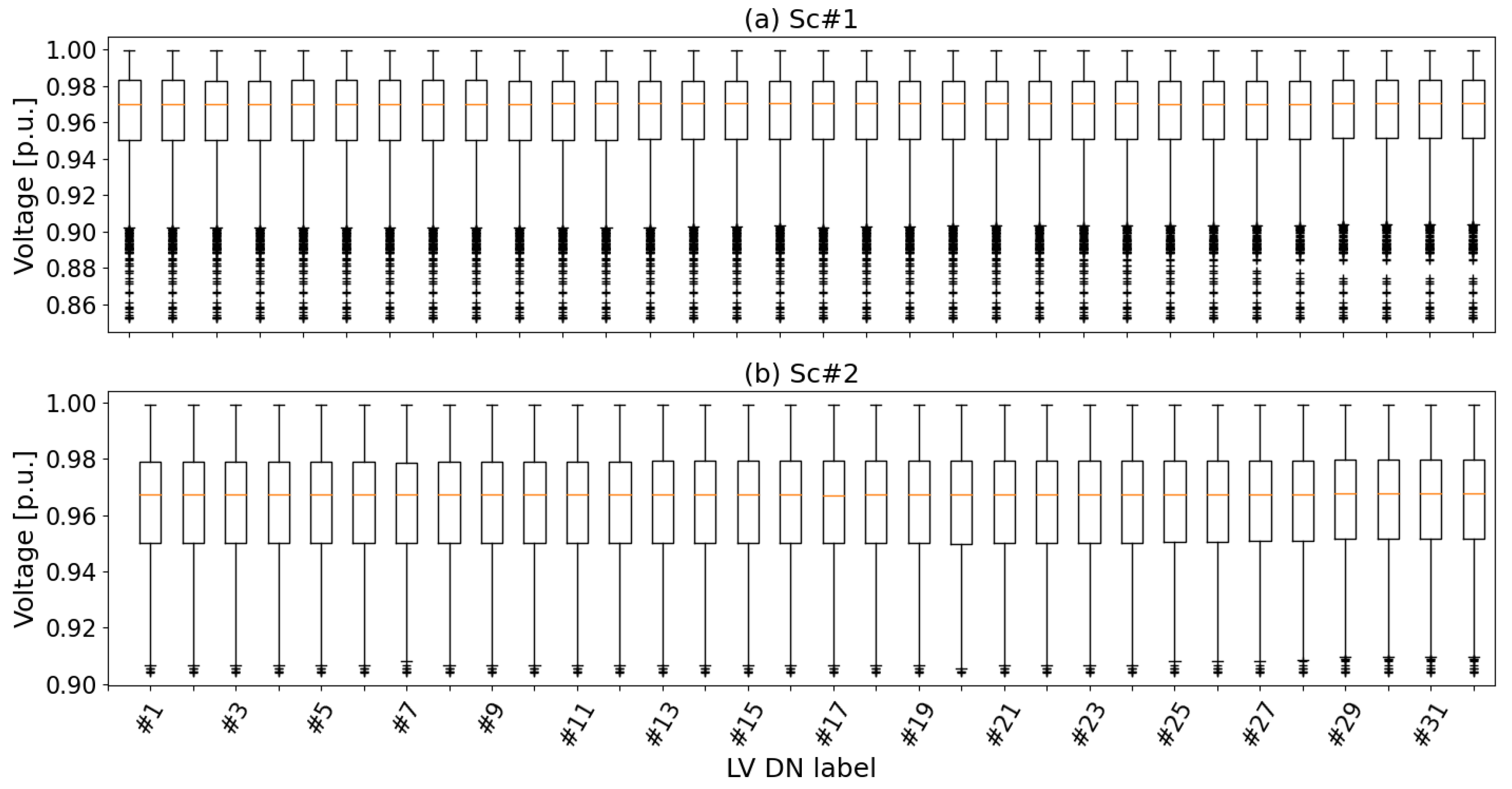
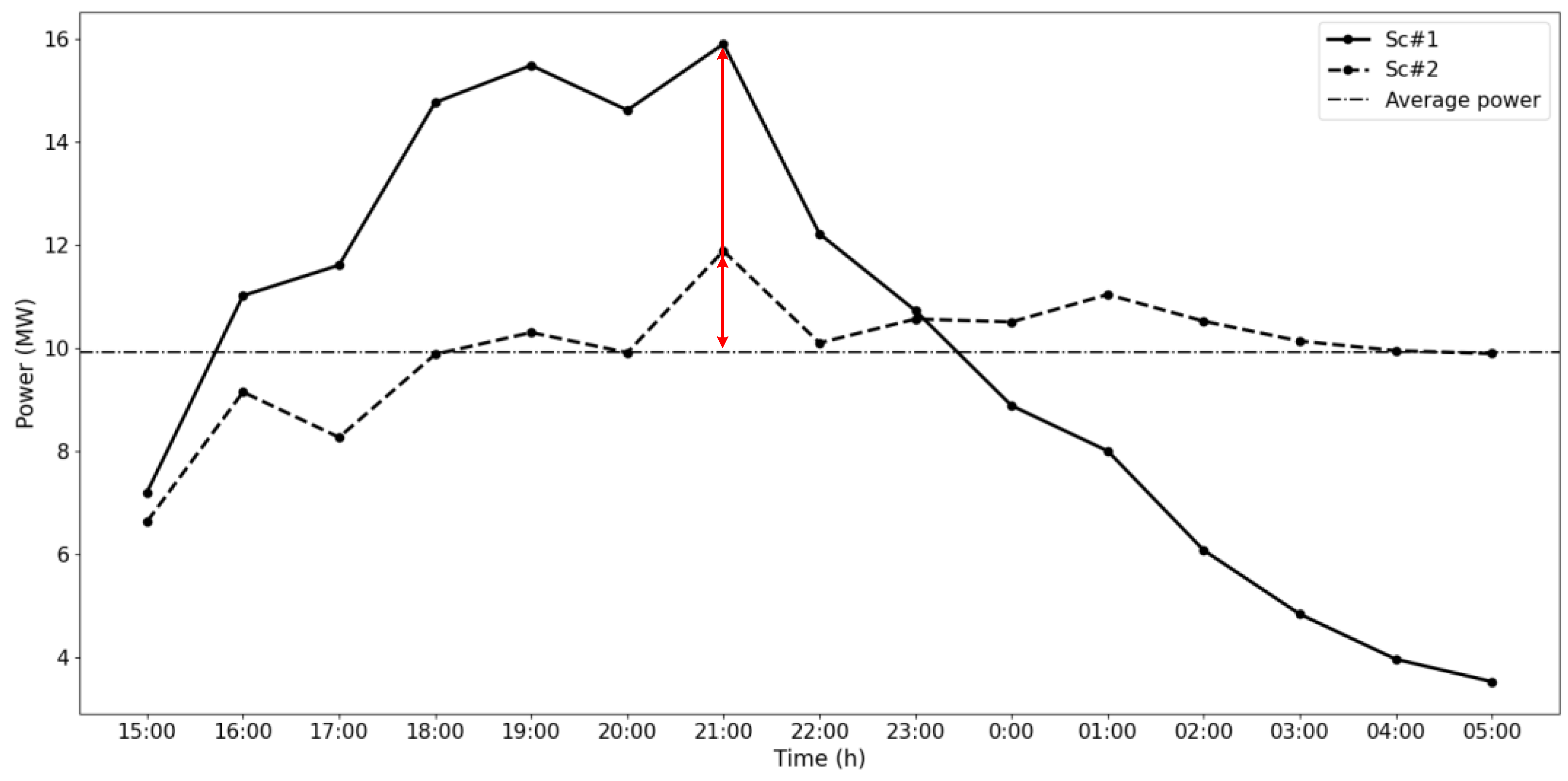
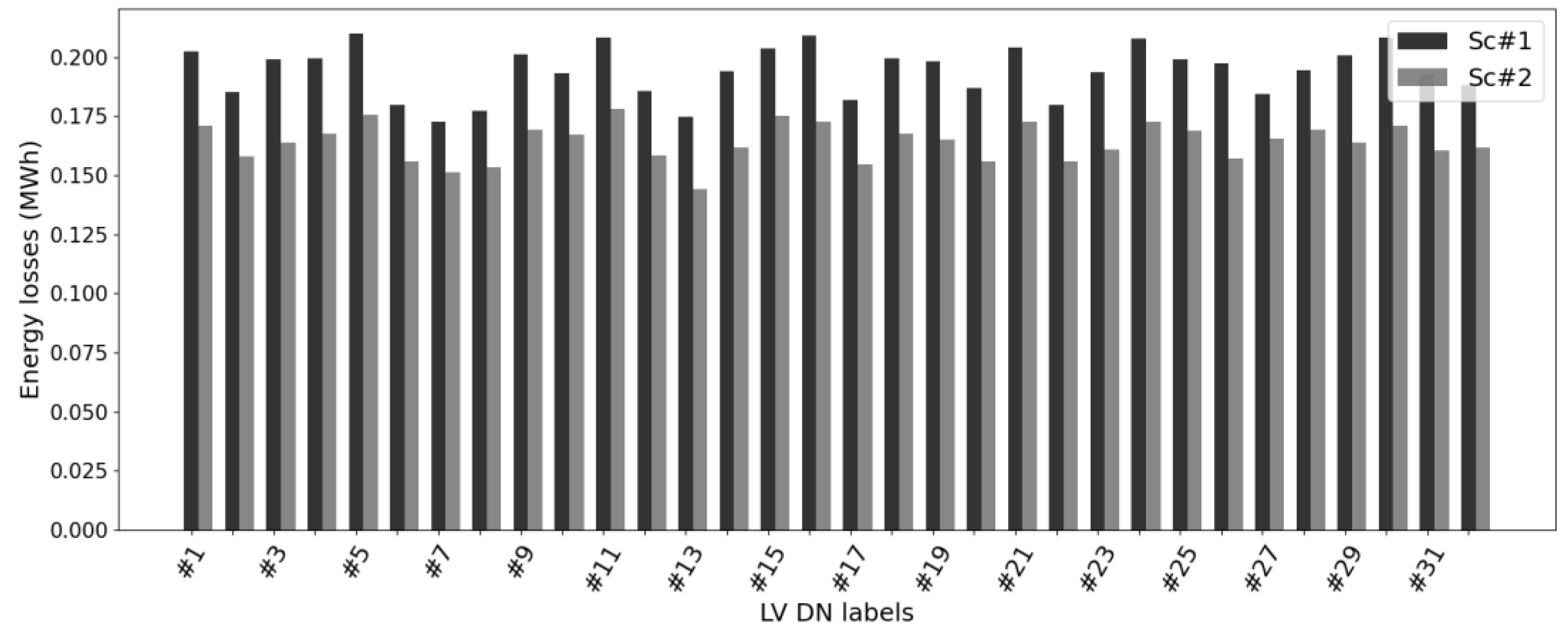
• Sc#1: This is the base scenario at which the EVs start charging by the time of their arrival and until they are fully charged. Thus, no charging planning is applied in this case.
• Sc#2: In this scenario, the proposed EVs’ charging planning methodology is applied.

Since we aim to examine how the EVs’ charging scheduling affects the power losses at the MV level, we assume that the same LV DN is connected to each node of the MV DN. The proposed methodology is applied to each one LV DN and requires as inputs the time of arrival, the SoC and the technical characteristics of EVs. Considering that the examined network is a residential one, the proposed charging scheduling covers a time period from 15:00 to 06:00. This is because the EVs are expected to arrive at home sometime between 15:00 and 00:00. Therefore, the examined time period (15:00–06:00) is sufficient to ensure the fully charging of EVs. The selected interval of EVs’ time of arrival is verified by study [39] in which the driving behavior of the EV owners is presented, and also verified by the data analysis conducted by Adaptive Charging Network Portal [40]. In this study, 32 LV DNs have been considered. Thus, for sake of illustration, the distributions of time of arrival for two LV DNs, i.e., LV#6 and LV#10, are presented in Figure 4. Additionally, the technical characteristics of the EVs are obtained from real EV models., i.e., battery capacity of 19 real EV models alongside with their chargers’ power, as presented in research [38]. The EVs’ have been randomly assigned to the residences. Finally, the SoC of EVs’ has been randomly set within the range of 20% to 40%. It should be clarified that the simulations and the results refer to BEV models. However, the type of EV, i.e., BEV or PHEV, does not affect the implementation of the proposed methodology.

The charging planning algorithm is executed-updated per hour, in case new arrivals are predicted. The impact of EV’s new arrivals to the charging planning of the already plugged-in EVs is presented in Figure 5. In Figure 5, each row illustrates the charging plan of one EV at each execution. Specifically, the green boxes indicate charging while the gray boxes denote idling. After each execution, the algorithm provides an updated charging plan based on the new information, i.e., new EVs arrival, SoC and car charger. Finally, the boxes with the blue frame indicate the final day ahead charging plan. As observed in Figure 5, this illustrated EV requires in total three hours to be charged. The initial charging planning (i.e., first row) allocates these hours sometime after midnight. The arrival of new EVs though at the next hour (i.e., second row) requires an update for the charging plan since the optimization problem needs to be solve again. This is performed at each hour with new arrivals, and this is why the charging plan at each hour is highly possible not be the one by the end of the examined time period.

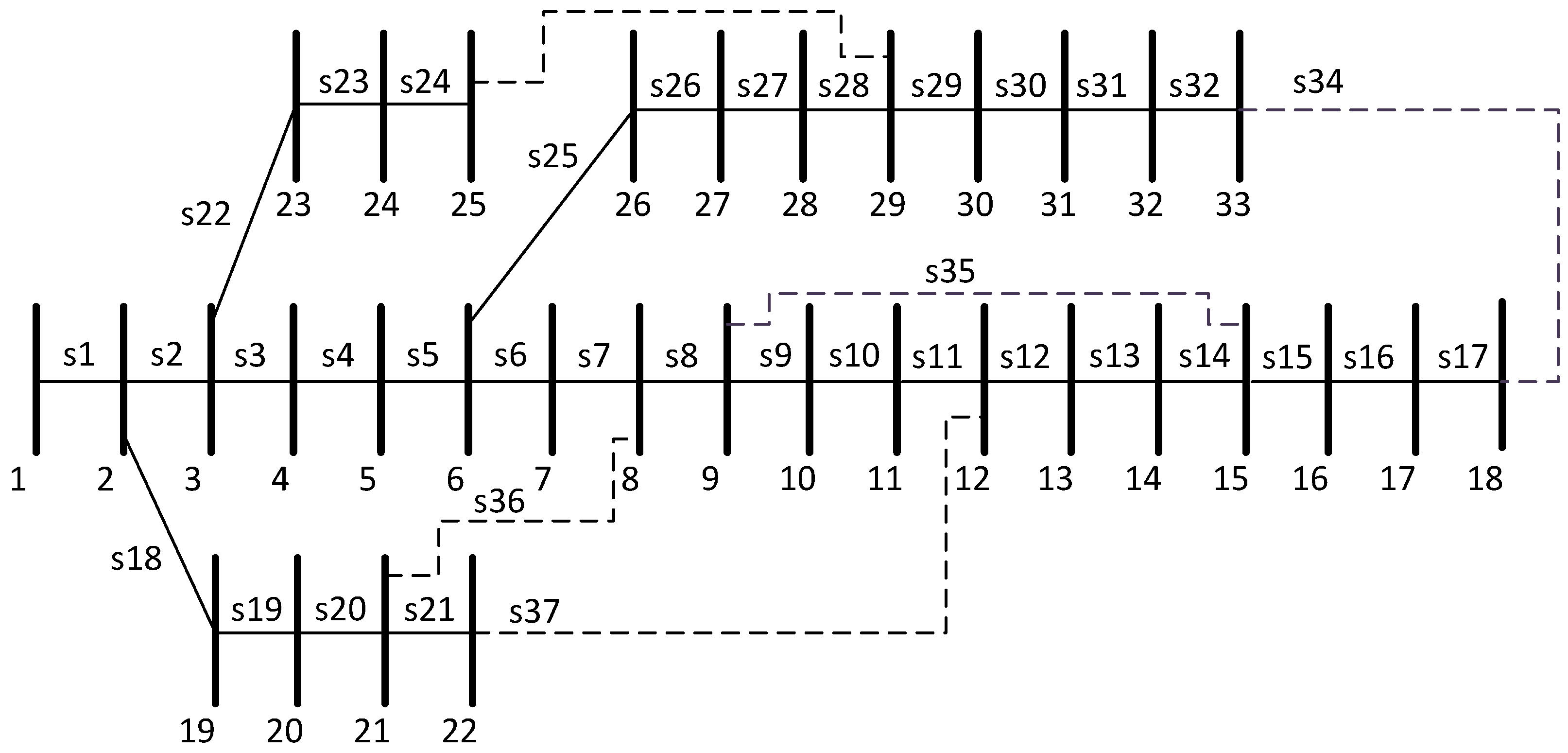
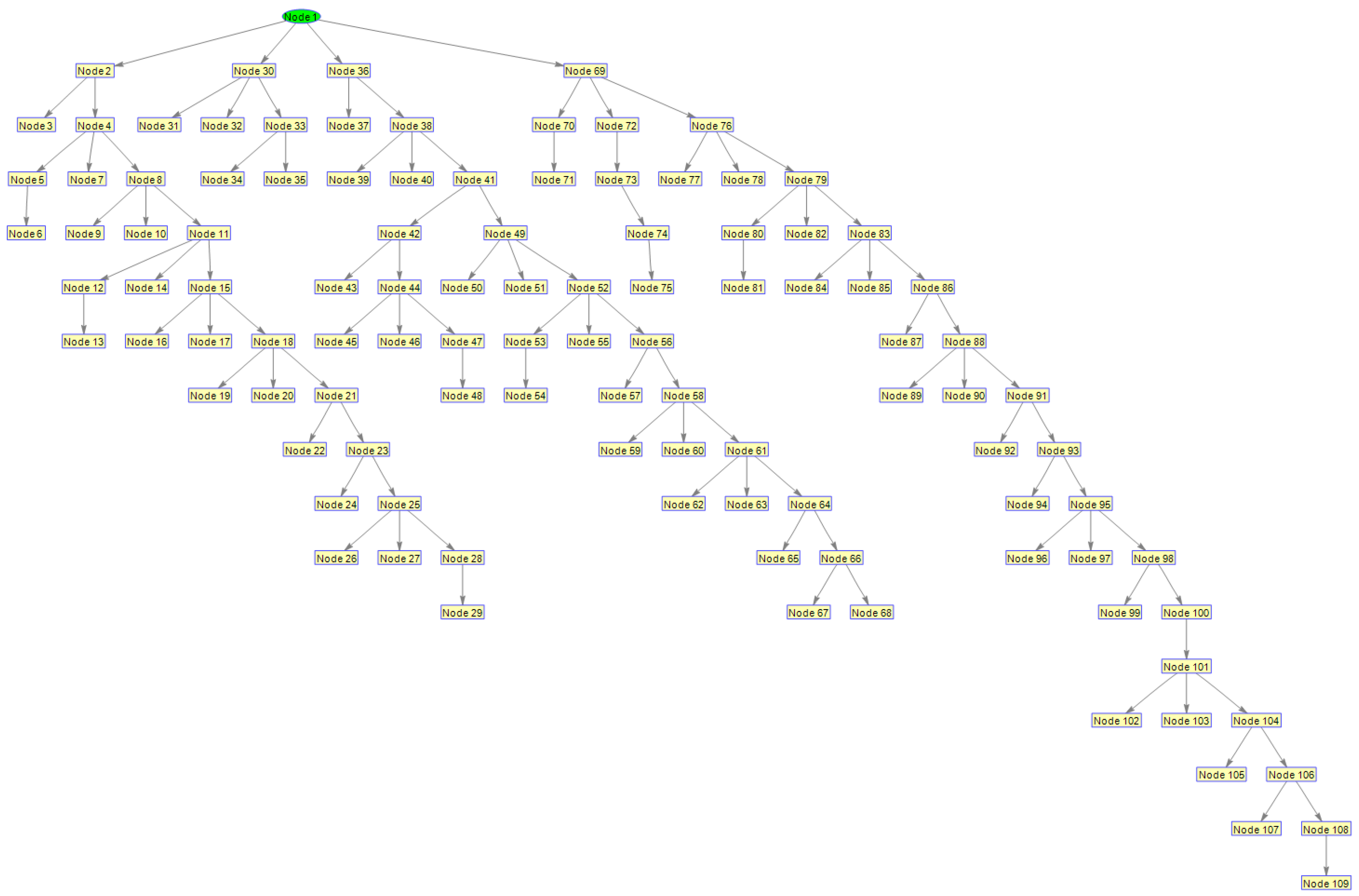
4.2. MV DN under Study

In order to assess the effectiveness of the proposed NR algorithm the IEEE 33-bus distribution system is utilized that operates at 12.99 kV. The system consists of 33 busses, 32 lines or sectionalizers (s1–s32) and 5, initially open, tie switches (s33–s37). The topology of the system is presented in Figure 6, where the dashed lines illustrate the tie switches. Although the IEEE 33-bus system has a total load size of 3.715 MW and 2.3 MVar, in our case this load is omitted. Instead, we assume that at busses 2–33 of the system a LV DN exists, the one of Figure 3 as presented in the previous subsection. The hourly load demand at each MV bus is the total hourly demand of the LV DN. This formulation is important since it captures for the first time (at least to the best of the authors knowledge) a detailed analysis of the load composition on the LV network and in turns it reflects these load variations at the MV network.

In order to estimate how the charging scheduling affects the power losses at the MV level and assess the contribution of NR towards power loss minimization in MV DN, four different scenarios have been implemented:

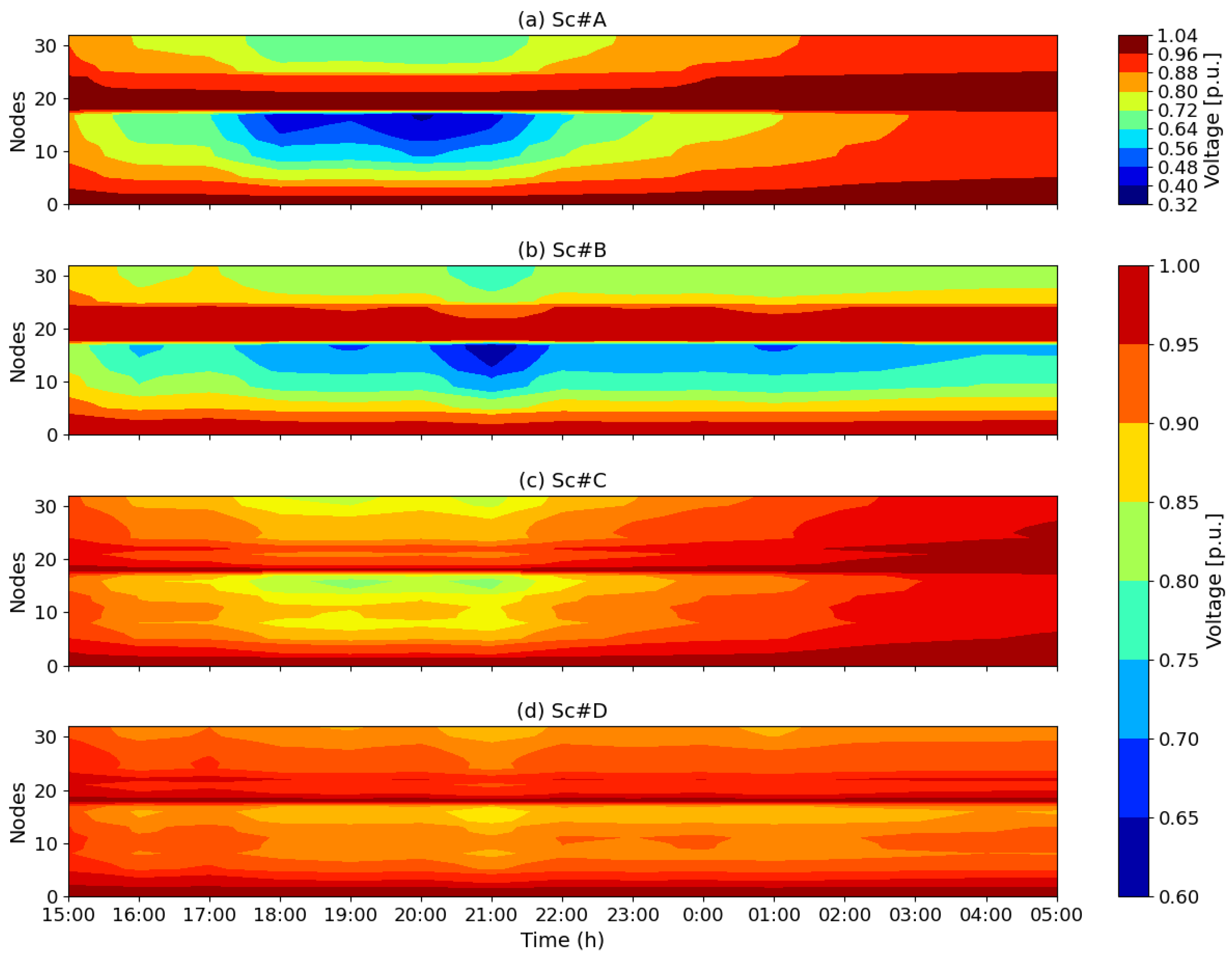
• Sc#A: This is the base scenario in which NR and charging scheduling are not applied to the MV and LV DNs, respectively.
• Sc#B: In this scenario, NR is not applied to MV DN. However, the EV charging scheduling is applied to LV DN. The aim here is to investigate how the load demand smoothing in the LV side network could contribute to reducing power losses also in the MV network.
• Sc#C: In this scenario, the NR is applied at MV DN, while the EVs charging is not considered.
• Sc#D: Both NR and charging scheduling are applied to MV and LV DNs, respectively.

4.3. Results at LV DN

In this subsection, the results of the proposed EV charging scheduling methodology are presented. The proposed methodology has been applied to 32 LV DNs since, as mentioned earlier, the LV network is considered to be connected to each MV node. Figure 7 presents the power losses of the LV DNs for Sc#1 and Sc#2, i.e., with and without the employment of EVs’ charging planning for a time period of one day. The employment of the proposed methodology can lead to a power loss reduction between 10.25% and 20.35%. Additionally,

Table 4. Results of average power loss reduction for the 32 LV DNs.

Scenario	Power Losses (MWh)	Loss Reduction% (in Respect to Sc#1)	SD
Sc#1	0.1941	-	-
Sc#2	0.1639	15.49	0.020

includes the average power losses for the 32 LV DNs, the average percentage of power loss reduction and the standard deviation (SD) of the percentage reduction. The results presented in Table 4 highlight the efficiency of the proposed methodology, since scenario Sc#2 can yield up to a 15.48% power loss reduction on average.

Furthermore, for both scenarios, the voltage profiles of the LV DNs have been assessed. Specifically, Figure 8 presents the boxplots of the voltage values of each LV DN for the total examined time period. In both scenarios, 75% of the observations are within the acceptable voltage limits, i.e., 0.95–1 p.u., while 25% of the observations lie within the range 0.9–0.95 p.u. However, from Figure 8a, it is clear that the uncoordinated charging of EVs can result in a prohibitive voltage drop, since many outliers with values less than 0.95% are detected. To this point, the proposed methodology deals with extensive voltage drop issues, since the outliers’ values are below 0.90 p.u. (Figure 8b).

Finally, Figure 9 presents the hourly total power demand of the LV DNs for each scenario, as well as the average demand. From Figure 9, we can conclude that the uncoordinated charging of EVs leads to charging overlaps and therefore to power demand increase at certain hours. In addition, the employment of the proposed charging planning of EVs can result to a smoother load curve, by minimizing the peaks and filling the valleys. In order to sufficiently compare the two load curves, the load factor (LF) indicator is utilized. LF, as expressed in (7), is the ratio of the average power demand ($P_{avg}$) of the examined period to the maximum power demand ($P_{max}$) occurred. The results point out that the optimal charging plan can achieve an LF increment of 33.71%.

$$\mathrm{L}\mathrm{F}=\frac{P_{avg}}{P_{max}}$$

(13)

4.4. Results at MV and LV DN

In

Table 5. Results of the proposed methodology.

	Power Losses at MV DN (MWh)	Power Losses at LV DN (MWh)	Total Power Losses (MWh)	Total Power Loss Reduction% (in Respect to Sc#A)	Minimum Voltage (p.u.)
Sc#A	34.61	6.211	40.821	-	0.387
Sc#B	22.97	5.246	28.216	30.88	0.610
Sc#C	11.701	6.211	17.912	56.12	0.815
Sc#D	9.598	5.246	14.843	63.64	0.864

, the results of the examined scenarios are presented, including the power losses for both the LV and MV levels. Considering Sc#A, which is the base scenario, the uncoordinated charging of EVs combined with the absence of NR can lead to extensive power losses and prohibited voltage values, i.e., the lowest voltage occurred is 0.387 p.u. Moreover, when only the EVs charging planning is applied to LV DNs (Sc#B) the power losses can be decreased by 30.88%. Yet, the lowest voltage is 0.61 p.u. Additionally, the employment of NR without the charging scheduling (Sc#C) can reduce the power losses by 56.12% and considerably improve the voltage of the system. Finally, the employment of the proposed methodology (Sc#D), that includes both NR and EV charging scheduling, can significantly decrease the power losses by 63.64% and result to further voltage improvement. It should be clarified that in scenarios Sc#C and Sc#D the optimal topology of the network is the same, as presented at

Table 6. Open sectionalizers/tie switches.

	Open Sectionalizers/Tie Switches
Sc#A	s30, s31, s32, s33, s34
Sc#B	s30, s31, s32, s33, s34
Sc#C	s9, s14, s17, s25, s31
Sc#D	s9, s14, s17, s25, s31

, although the hourly load of each node differs, as illustrated in Figure 10.

The performance of the proposed methodology is additionally assessed in terms of voltage profile improvement. In Figure 11, the voltage profile of each scenario for the examined time period is presented. From Figure 11a, it is clear that for Sc#A the system experiences intense voltage drops at afternoon hours. Even if the employment of EVs’ charging scheduling without considering NR (Sc#B) can improve the voltage profile, intense voltage drops are still occurred as presented in Figure 11b. Considering Figure 11c,d, the employment of NR method can significantly improve the voltage profile. Finally, Figure 11d points out the efficiency of the proposed methodology, i.e., employment of both EVs’ charging scheduling and NR.

5. Conclusions

In this paper, a two-stage EV charging scheduling and NR methodology is proposed, addressing the issue of power loss reduction in LV and MV DN, respectively. In the first stage, the charging planning is employed considering the key role of an aggregator. Specifically, the aggregator, which is responsible for a LV DN, applies the EV charging scheduling, in order to reduce the power losses of the network, and provides an optimal day-ahead charging plan. The proposed charging planning is applied every hour of the examined time horizon in case new arrivals are predicted and provides an updated charging schedule for the remaining time period. In the second stage, the DSO applies the NR to MV DN, in order to determine the optimal day-ahead topology of the system. The NR is executed considering the hourly day-ahead demand, as formulated by the aggregators.

The results of the proposed methodology are assessed at the LV level and MV level, respectively. The results highlight that:

• At the LV level, the coordinated charging of EVs can lead to a power loss reduction between 10.25% and 20.35%.
• At the MV level, the employment of charging scheduling can decrease the power losses of MV DN by 30.88%.
• The employment of both charging scheduling and NR results in a significant power loss reduction of 63.64%.

References

1. European Comission. Directive of the European Parliament and of the Council on Energy Efficiency (Recast). 2021/0203(COD); European Comission: Brussels, Belgium, 2021; Available online: https://eur-lex.europa.eu/legal-content/EN/TXT/?uri=Celex:52021PC0558 (accessed on 15 January 2002).
2. Directive 2012/27/EU of the European Parliament and of the Council of 25 October 2012 on Energy Efficiency, Amending Directives 2009/125/EC and 2010/30/EU and repealing Directives 2004/8/EC and 2006/32/EC. Off. J. Eur. Union 2012. Available online: https://eur-lex.europa.eu/legal-content/EN/TXT/PDF/?uri=CELEX:32012L0027&from=en (accessed on 15 January 2002).
3. Council of European Energy Regulators (CEER). 2nd CEER Report on Energy Losses; CEER: Brussels, Belgium, 2020; Available online: https://www.ceer.eu/documents/104400/-/-/fd4178b4-ed00-6d06-5f4b-8b87d630b060 (accessed on 15 January 2002).
4. Bompard, E.; Serrenho, T.; Bertoldi, P.; European Commission. Improving Energy Efficiency in Electricity Networks: Addressing Network Losses & EU regulations under Article 15 (2) (a) of the Energy Efficiency Directive. 2020. Available online: https://op.europa.eu/en/publication-detail/-/publication/f5d89f60-344e-11eb-b27b-01aa75ed71a1 (accessed on 15 January 2002).
5. European Union Agency for the Cooperation of Energy Regulators (ACER). Report on Distribution Tariff Methodologies in Europe. 2021. Available online: https://documents.acer.europa.eu/Official_documents/Acts_of_the_Agency/Publication/ACER%20Report%20on%20D-Tariff%20Methodologies.pdf (accessed on 16 January 2002).
6. European Commission. Communication from the Commission: The European Green Deal. COM(2019) 640 Final; European Commission: Brussels, Belgium, 2019; Available online: https://eur-lex.europa.eu/legal-content/EN/TXT/?qid=1576150542719&uri=COM%3A2019%3A640%3AFIN (accessed on 16 January 2002).
7. Wróblewski, P.; Drożdż, W.; Lewicki, W.; Dowejko, J. Total Cost of Ownership and Its Potential Consequences for the Development of the Hydrogen Fuel Cell Powered Vehicle Market in Poland. Energies 2021, 14, 2131. [Google Scholar] [CrossRef]
8. Wróblewski, P.; Kupiec, J.; Drożdż, W.; Lewicki, W.; Jaworski, J. The Economic Aspect of Using Different Plug-In Hybrid Driving Techniques in Urban Conditions. Energies 2021, 14, 3543. [Google Scholar] [CrossRef]
9. EV and EV Charger Incentives in Europe: A Complete Guide for Businesses and Individuals. Available online: https://blog.wallbox.com/ev-incentives-europe-guide/#index_5 (accessed on 17 January 2002).
10. Hussain, M.T.; Bin Sulaiman, N.; Jabir, M. Optimal Management strategies to solve issues of grid having Electric Vehicles (EV): A review. J. Energy Storage 2021, 33, 102114. [Google Scholar] [CrossRef]
11. Wu, Y.; Wang, Z.; Huangfu, Y.; Ravey, A.; Chrenko, D.; Gao, F. Hierarchical Operation of Electric Vehicle Charging Station in Smart Grid Integration Applications—An Overview. Int. J. Electr. Power Energy Syst. 2022, 139, 108005. [Google Scholar] [CrossRef]
12. Bouhouras, A.S.; Gaidatzis, P.P.; Labridis, D. Handbook of Optimization in Electric Power Distribution Systems; Springer: Berlin/Heidelberg, Germany, 2020. [Google Scholar]
13. Kothona, D.; Bouhouras, A.S.; Skalidi, I.; Gkaidatzis, P.; Poulakis, N.; Christoforidis, G.C. EV Flexibility Contribution to Distribution Network Operation. In Proceedings of the 12th Mediterranean Conference on Power Generation, Transmission, Distribution and Energy Conversion (MEDPOWER 2020), Paphos, Cyprus, 9–12 November 2020. [Google Scholar]
14. Helmi, A.M.; Carli, R.; Dotoli, M.; Ramadan, H.S. Efficient and Sustainable Reconfiguration of Distribution Networks via Metaheuristic Optimization. IEEE Trans. Autom. Sci. Eng. 2021, 19, 82–98. [Google Scholar] [CrossRef]
15. Abdul, W.I.A.B.W.; Saedi, A.B.; Peeie, M.H.B.; Hanifah, M.S.B.A. Modeling of the Network Reconfiguration Considering Electric Vehicle Charging Load. In Proceedings of the 2021 8th International Conference on Computer and Communication Engineering (ICCCE), Kuala Lumpur, Malaysia, 22–23 June 2021. [Google Scholar]
16. Salkuti, S.R. Network Reconfiguration of Distribution System with Distributed Generation, Shunt Capacitors and Electric Vehicle Charging Stations. In Next Generation Smart Grids: Modeling, Control and Optimization. Lecture Notes in Electrical Engineering; Springer: Singapore, 2022. [Google Scholar]
17. Sun, Q.; Yu, Y.; Li, D.; Hu, X. A distribution network reconstruction method with DG and EV based on improved gravitation algorithm. Syst. Sci. Control Eng. 2020, 9, 6–13. [Google Scholar] [CrossRef]
18. Jangdoost, A.; Keypour, R.; Golmohamadi, H. Optimization of distribution network reconfguration by a novel RCA integrated with genetic algorithm. Energy Syst. 2021, 12, 801–833. [Google Scholar] [CrossRef]
19. Pahlavanhoseini, A.; Sepasian, M.S. Scenario-based planning of fast charging stations considering network reconfiguration using cooperative coevolutionary approach. J. Energy Storage 2019, 23, 544–557. [Google Scholar] [CrossRef]
20. Ahmad, F.; Iqbal, A.; Ashraf, I.; Marzband, M.; Khan, I. Optimal location of electric vehicle charging station and its impact on distribution network: A review. Energy Rep. 2022, 8, 2314–2333. [Google Scholar] [CrossRef]
21. Nour, M.; Chaves-Ávila, J.P.; Magdy, G.; Sánchez-Miralles, Á. Review of Positive and Negative Impacts of Electric Vehicles Charging on Electric Power Systems. Energies 2020, 13, 4675. [Google Scholar] [CrossRef]
22. Van Kriekinge, G.; De Cauwer, C.; Sapountzoglou, N.; Coosemans, T.; Messagie, M. Peak shaving and cost minimization using model predictive control for uni- and bi-directional charging of electric vehicles. Energy Rep. 2021, 7, 8760–8771. [Google Scholar] [CrossRef]
23. Tu, R.; Gai, Y.J.; Farooq, B.; Posen, D.; Hatzopoulou, M. Electric vehicle charging optimization to minimize marginal greenhouse gas emissions from power generation. Appl. Energy 2020, 277, 115517. [Google Scholar] [CrossRef]
24. Wang, J.; Wang, W.; Wang, H.; Zuo, H. Dynamic Reconfiguration of Multiobjective Distribution Networks Considering DG and EVs Based on a Novel LDBAS Algorithm. IEEE Access 2020, 8, 216873–216893. [Google Scholar] [CrossRef]
25. Cheng, S.; Li, Z. Multi-objective Network Reconfiguration Considering V2G of Electric Vehicles in Distribution System with Renewable Energy. Energy Procedia 2019, 158, 278–283. [Google Scholar] [CrossRef]
26. Rostami, M.-A.; Kavousi-Fard, A.; Niknam, T. Expected Cost Minimization of Smart Grids with Plug-In Hybrid Electric Vehicles Using Optimal Distribution Feeder Reconfiguration. IEEE Trans. Ind. Inform. 2015, 11, 388–397. [Google Scholar] [CrossRef]
27. Singh, J.; Tiwari, R. Active and Reactive Power Management of EVs in Reconfigurable Distribution System. In Proceedings of the 2020 IEEE 9th Power India International Conference (PIICON), Sonepat, India, 28 February–1 March 2020. [Google Scholar]
28. Sedighizadeh, M.; Shaghaghi-Shahr, G.; Esmaili, M.; Aghamohammadi, M.R. Optimal distribution feeder reconfiguration and generation scheduling for microgrid day-ahead operation in the presence of electric vehicles considering uncertainties. J. Energy Storage 2018, 21, 58–71. [Google Scholar] [CrossRef]
29. Singh, J.; Tiwari, R. Real power loss minimisation of smart grid with electric vehicles using distribution feeder reconfiguration. IET Gener. Transm. Distrib. 2019, 13, 4249–4261. [Google Scholar] [CrossRef]
30. Amin, A.; Tareen, W.U.K.; Usman, M.; Memon, K.A.; Horan, B.; Mahmood, A.; Mekhilef, S. An Integrated Approach to Optimal Charging Scheduling of Electric Vehicles Integrated with Improved Medium-Voltage Network Reconfiguration for Power Loss Minimization. Sustainability 2020, 12, 9211. [Google Scholar] [CrossRef]
31. EN. Directive (EU) 2018/844 of the European Parliament and of the Council of 30 May 2018 amending Directive 2010/31/EU on the energy performance of buildings and Directive 2012/27/EU on energy efficiency. Off. J. Eur. Union 2018, 156, 75–91. [Google Scholar]
32. Kerscher, S.; Arboleya, P. The key role of aggregators in the energy transition under the latest European regulatory framework. Int. J. Electr. Power Energy Syst. 2021, 134, 107361. [Google Scholar] [CrossRef]
33. Carli, R.; Dotoli, M. A Distributed Control Algorithm for Waterfilling of Networked Control Systems via Consensus. IEEE Control Syst. Lett. 2017, 1, 334–339. [Google Scholar] [CrossRef]
34. Carli, R.; Dotoli, M. A Distributed Control Algorithm for Optimal Charging of Electric Vehicle Fleets with Congestion Management. IFAC PapersOnLine 2018, 51, 373–378. [Google Scholar] [CrossRef]
35. Parise, F.; Grammatico, S.; Gentile, B.; Lygeros, J. Distributed convergence to Nash equilibria in network and average aggregative games. Automatica 2020, 117, 108959. [Google Scholar] [CrossRef]
36. Jahangir, H.; Tayarani, H.; Ahmadian, A.; Golkar, M.A.; Miret, J.; Tayarani, M.; Gao, H.O. Charging demand of Plug-in Electric Vehicles: Forecasting travel behavior based on a novel Rough Artificial Neural Network approach. J. Clean. Prod. 2019, 229, 1029–1044. [Google Scholar] [CrossRef]
37. Gkaidatzis, P.A.; Doukas, D.I.; Labridis, D.P.; Bouhouras, A.S. Comparative analysis of heuristic techniques applied to ODGP. In Proceedings of the 2017 17th IEEE International Conference on Environment and Electrical Engineering and 2017 1st IEEE Industrial and Commercial Power Systems Europe, EEEIC/I and CPS Europe 2017, Milan, Italy, 6–9 June 2017. [Google Scholar]
38. Bouhouras, A.S.; Kothona, D.; Gkaidatzis, P.A.; Christoforidis, G.C. Distribution network energy loss reduction under EV charging schedule. Int. J. Energy Res. 2022, 46, 8256–8270. [Google Scholar] [CrossRef]
39. Zhang, J.; Yan, J.; Liu, Y.; Zhang, H.; Lv, G. Daily electric vehicle charging load profiles considering demographics of vehicle users. Appl. Energy 2020, 274, 115063. [Google Scholar] [CrossRef]
40. Adaptive Charging Network Research Portal. Available online: https://ev.caltech.edu/index (accessed on 24 February 2021).
Figure 1. Illustration of an example of the algorithm’s execution.
Energies 15 03808 g001
Figure 2. Flowchart of the proposed methodology.
Energies 15 03808 g002
Figure 3. Low-voltage distribution network.
Energies 15 03808 g003
Figure 4. Probability distribution of EVs’ time of arrival.
Energies 15 03808 g004
Figure 5. EVs’ updated charging plan due to new arrival forecasts.
Energies 15 03808 g005
Figure 6. IEEE 33-bus system.
Energies 15 03808 g006
Figure 7. Power losses at each distribution system.
Energies 15 03808 g007
Figure 8. Boxplots of voltage values of all nodes within the examined time period for (a) Sc#1 and (b) Sc#2.
Energies 15 03808 g008
Figure 9. Load curves of the total hourly power demand.
Energies 15 03808 g009
Figure 10. Load demand for: (a) Sc#C, (b) Sc#D.
Energies 15 03808 g010
Figure 11. MV DN voltage profile for: (a) Sc#A, (b) Sc#B, (c) Sc#C and (d) Sc#D.
Energies 15 03808 g011