
Modeling Differential Pressure of Diesel Particulate Filters in Marine Engines

 ,
,  , ,
, ,
Abstract
:1. Introduction
2. Experiment
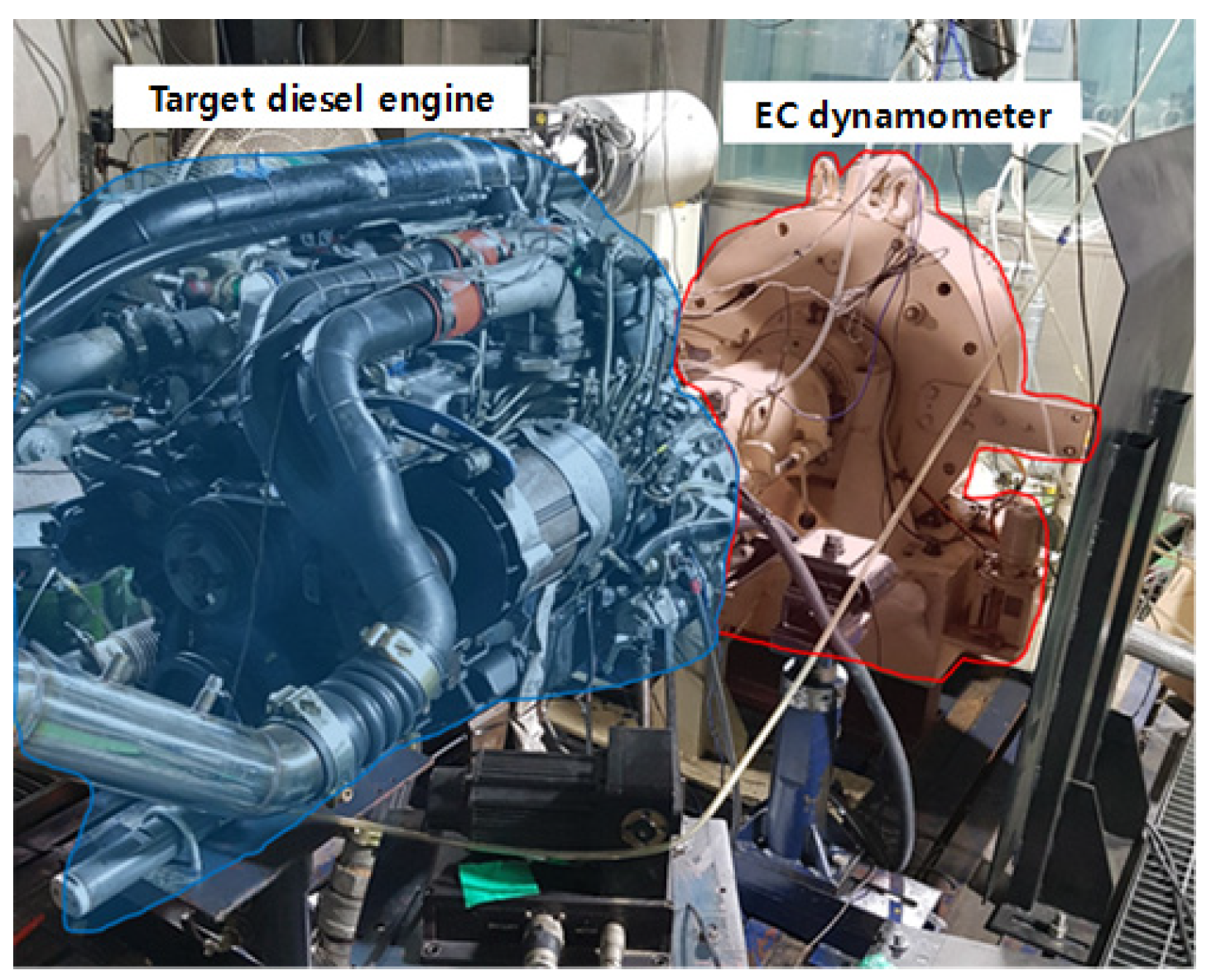
2.1. Experimental Apparatus
2.1.1. Specification of Marine Engine
2.1.2. Diesel Particulate Filter (DPF)
2.2. Differential Pressure Test
2.2.1. Experimental Conditions
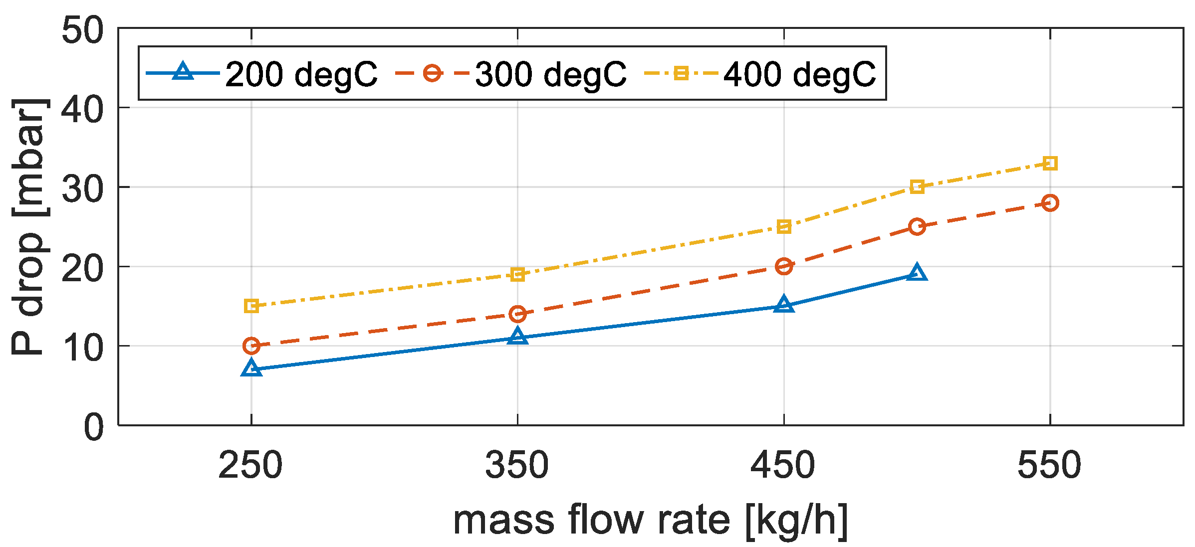
2.2.2. Zero PM Condition
2.3. Effect of Captured PM
2.3.1. PM Capture
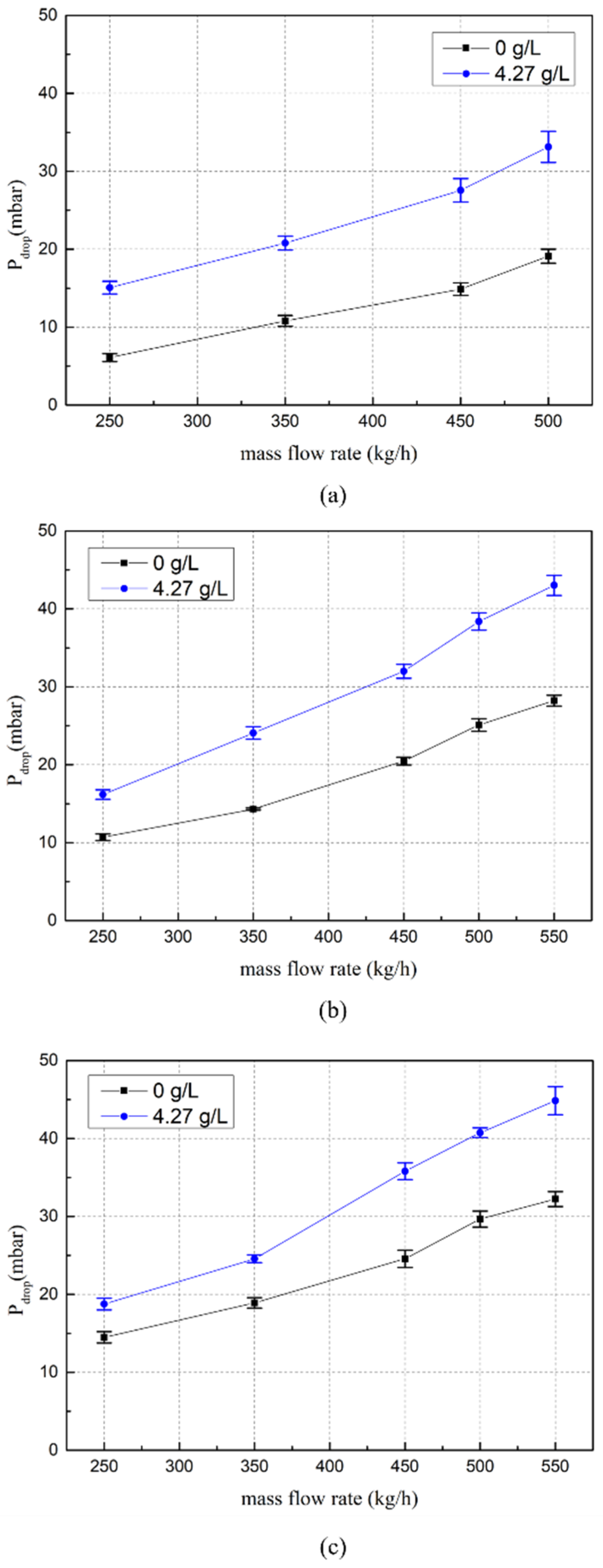
2.3.2. Differential Pressure Test with PM Capture
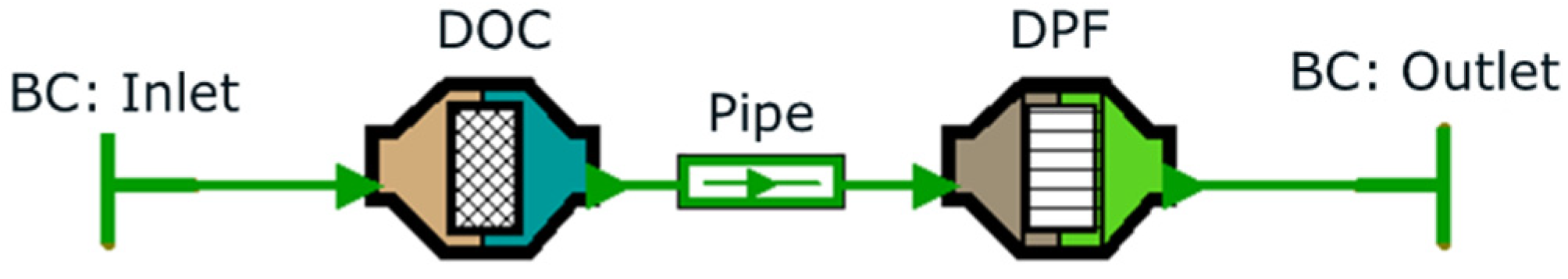
3. Modeling of Differential Pressure Model
3.1. Differential Pressure Model
3.2. Clean DPF Modeling
Soot Loading
3.3. Differential Pressure at High Soot Loading
4. Conclusions
Author Contributions
Funding
Institutional Review Board Statement
Informed Consent Statement
Data Availability Statement
Conflicts of Interest
References
- Jung, S.C.; Park, J.S.; Yoon, W.S. Rigorous Modeling of Single Channel DPF Filtration and Sensitivity Analysis of Important Model Parameters. Trans. KSAE 2006, 14, 127–136. [Google Scholar]
- Yu, J.; Chun, J.R.; Hong, H.J. Prediction of Particulate Matter Being Accumulated in a Diesel Particulate Filter. Trans. KSAE 2009, 17, 29–34. [Google Scholar]
- Bissett, E.J. Mathematical Model of the Thermal Regeneration of a Wall-flow Monolith Diesel Particulate Filter. Chem. Eng. Sci. 1984, 39, 1233–1244. [Google Scholar] [CrossRef]
- Jung, S.C.; Park, J.S.; Yoon, W.S. Rigorous Modeling of Pressure Drops for Single Channel DPF Filtration. SAE Technical Papers. Gyunggido, Korea. 24–26 November 2005, pp. 408–415. Available online: https://www.dbpia.co.kr/journal/articleDetail?nodeId=NODE00660013 (accessed on 10 May 2022).
- Mizutani, T.; Watanabe, Y.; Yuuki, K.; Hashimoto, S.; Hamanaka, T.; Kawashima, J. Soot Regeneration Model for SiC-DPF System Design. In Proceedings of the SAE 2004 World Congress & Exhibition, Detroit, MI, USA, 8–11 March 2004. [Google Scholar] [CrossRef]
- Lee, S.J.; Jeong, S.J.; Kim, W.S. Numerical Design of the Diesel Particulate Filter for Optimum Thermal Performances during Regeneration. Appl. Energy 2009, 86, 1124–1135. [Google Scholar] [CrossRef]
- Khan, M.R.; Shamim, T. Regeneration Characteristics of Diesel Particulate Filters Under Transient Exhaust Conditions. In Proceedings of the International Combustion Engine Division Spring Technical Conference, Chicago, IL, USA, 27–30 April 2008; pp. 107–115. [Google Scholar]
- Ogyu, K.; Ohno, K.; Hong, S.; Komori, T. Ash Storage Capacity Enhancement of Diesel Particulate Filter. SAE Trans. 2004, 113, 466–473. [Google Scholar]
- Huynh, C.T.; Johnson, J.H.; Yang, S.L.; Bagley, S.T.; Warner, J.R. A One-dimensional Computational Model for Studying the Filtration and Regeneration Characteristics of a Catalyzed Wall-flow Diesel Particulate Filter. SAE Trans. 2003, 112, 620–646. [Google Scholar]
- Tan, J.C.; Opris, C.N.; Baumgard, K.J.; Johnson, J.H. A Study of the Regeneration Process in Diesel Particulate Traps Using a Copper Fuel Additive; Society of Automotive Engineers, Inc.: Warrendale, PA, USA, 1996. [Google Scholar]
- Koltsakis, G.; Haralampous, O.; Depcik, C.; Ragone, J.C. Catalyzed Diesel Particulate Filter Modeling. Chem. Eng. 2013, 29, 1–61. [Google Scholar] [CrossRef] [Green Version]
- Punke, A.; Grubert, G.; Li, Y.; Dettling, J.; Neubauer, T. Catalyzed Soot Filters in Close Coupled Position for Passenger Vehicles. In Proceedings of the SAE 2006 World Congress & Exhibition, Detroit, MI, USA, 3–6 April 2006. [Google Scholar] [CrossRef]
- Kuwahara, T.; Yoshida, K.; Kuroki, T.; Hanamoto, K.; Sato, K.; Okubo, M. High Reduction Efficiencies of Adsorbed NOx in Pilot-Scale Aftertreatment Using Nonthermal Plasma in Marine Diesel-Engine Exhaust Gas. Energies 2019, 12, 3800. [Google Scholar] [CrossRef] [Green Version]
- Zokoe, J.; Su, C.; McGinn, P.J. Soot Combustion Activity and Potassium Mobility in Diesel Particulate Filters Coated with a K-Ca-Si-O Glass Catalyst. Ind. Eng. 2019, 58, 11891–11901. [Google Scholar] [CrossRef]
- Engelmann, D.; Zimmerli, Y.; Czerwinski, J.; Bonsack, P. Real Driving Emissions in Extended Driving Conditions. Energies 2021, 14, 7310. [Google Scholar] [CrossRef]
- Du, Y.; Hu, G.; Xiang, S.; Zhang, K.; Liu, H.; Guo, F. Estimation of the Diesel Particulate Filter Soot Load Based on an Equivalent Circuit Model. Energies 2018, 11, 472. [Google Scholar] [CrossRef] [Green Version]
- Ge, J.C.; Choi, N.J. Soot Particle Size Distribution Regulated and Unregulated Emissions of a Diesel Engine Fueled with Palm Oil Biodiesel Blends. Energies 2020, 13, 5736. [Google Scholar] [CrossRef]
- Jarosiński, W.; Wiśniowski, P. Verifying the Efficiency of a Diesel Particulate Filter Using Particle Counters with Two Different Measurements in Periodic Technical Inspection of Vehicles. Energies 2021, 14, 5128. [Google Scholar] [CrossRef]
- Verma, P.; Stevanovic, S.; Zare, A.; Dwivedi, G.; Chu Van, T.; Davidson, M.; Rainey, T.; Brown, R.J.; Ristovski, Z.D. An Overview of the Influence of Biodiesel, Alcohols and Various Oxygenated Additives on the Particulate Matter Emissions from Diesel Engines. Energies 2019, 12, 1987. [Google Scholar] [CrossRef] [Green Version]
- Beller, G.; Arpad, I.; Kiss, J.T.; Kocsis, D. AVL BOOST: A Powerful Tool for Research and Education. J. Phys. Conf. Ser. 1935, 012015. [Google Scholar] [CrossRef]
- Wirojsakunchai, E.; Schroeder, E.; Kolodziej, C.; Foster, D.E.; Schmidt, N.; Root, T.; Kawai, T.; Suga, T.; Nevius, T.; Kusaka, T. Detailed Diesel Exhaust Particulate Characterization and Real-Time DPF Filtration Efficiency Measurements During PM Filling Process. In Proceedings of the SAE World Congress & Exhibition, Detroit, MI, USA, 16–19 April 2007. [Google Scholar] [CrossRef]


| Variable | Value | Unit | |
|---|---|---|---|
| DPF | Filter type | Cordierite | |
| Cell density | 100 | CPSI | |
| Substrate wall thickness | 17.7 | mil | |
| Monolith diameter | 300 | mm | |
| Monolith length | 300 | mm | |
| Plug length | 20 | mm | |
| DOC | Filter type | Cordierite | |
| Cell density | 100 | CPSI | |
| Monolith diameter | 300 | mm | |
| Monolith length | 150 | mm | |
| DPF Inlet Temperature | Exhaust Mass Flow Rate | PM Mass | Differential Pressure |
|---|---|---|---|
| °C | kg/h | g/L | mbar |
| 200 | 250 | 0 | 7 |
| 350 | 11 | ||
| 450 | 15 | ||
| 500 | 19 | ||
| 550 | - | ||
| 300 | 250 | 10 | |
| 350 | 14 | ||
| 450 | 20 | ||
| 500 | 25 | ||
| 550 | 28 | ||
| 400 | 250 | 15 | |
| 350 | 19 | ||
| 450 | 25 | ||
| 500 | 30 | ||
| 550 | 33 |
| No. | Zero PM [kg] | 4.27 g/L PM Loaded [kg] |
|---|---|---|
| 1 | 85.893 | 85.979 |
| 2 | 85.876 | 85.961 |
| 3 | 85.872 | 85.967 |
| 4 | 85.878 | 85.985 |
| 5 | 85.883 | 85.985 |
| Average | 85.880 | 85.975 |
| DPF Inlet Temperature | Exhaust Mass Flow Rate | PM Load | Differential Pressure |
|---|---|---|---|
| ℃ | kg/h | g/L | mbar |
| 200 | 250 | 4.27 | 15 |
| 350 | 21 | ||
| 450 | 28 | ||
| 500 | 33 | ||
| 550 | - | ||
| 300 | 250 | 16 | |
| 350 | 24 | ||
| 450 | 32 | ||
| 500 | 38 | ||
| 550 | 43 |
| ζinl | 4.78 | |
| ζout | 2.64 | |
| kw | 200 | 6.23 × 10⁻¹¹ |
| 300 | 6.27 × 10⁻¹³ | |
| 400 | 4.48 × 10⁻¹³ | |
| Soot Packing Density | 100 kg/m3 | |
|---|---|---|
| ksc | 200 | 2.3 × 10⁻¹⁴ |
| 300 | 3.6 × 10⁻¹⁴ | |
| 400 | 5.9 × 10⁻¹⁴ | |
Publisher’s Note: MDPI stays neutral with regard to jurisdictional claims in published maps and institutional affiliations. |
© 2022 by the authors. Licensee MDPI, Basel, Switzerland. This article is an open access article distributed under the terms and conditions of the Creative Commons Attribution (CC BY) license (https://creativecommons.org/licenses/by/4.0/).
Share and Cite
Jang, J.; Min, B.; Ahn, S.; Kim, H.; Na, S.; Kang, J.; Roh, H.; Choi, G. Modeling Differential Pressure of Diesel Particulate Filters in Marine Engines. Energies 2022, 15, 3803. https://doi.org/10.3390/en15103803
Jang J, Min B, Ahn S, Kim H, Na S, Kang J, Roh H, Choi G. Modeling Differential Pressure of Diesel Particulate Filters in Marine Engines. Energies. 2022; 15(10):3803. https://doi.org/10.3390/en15103803
Chicago/Turabian StyleJang, Jaehwan, Byungchae Min, Seongyool Ahn, Hyunjun Kim, Sangkyung Na, Jeongho Kang, Heehwan Roh, and Gyungmin Choi. 2022. "Modeling Differential Pressure of Diesel Particulate Filters in Marine Engines" Energies 15, no. 10: 3803. https://doi.org/10.3390/en15103803
APA StyleJang, J., Min, B., Ahn, S., Kim, H., Na, S., Kang, J., Roh, H., & Choi, G. (2022). Modeling Differential Pressure of Diesel Particulate Filters in Marine Engines. Energies, 15(10), 3803. https://doi.org/10.3390/en15103803