What Is the Temporal Path of the GDP Elasticity of Energy Consumption in OECD Countries? An Assessment of Previous Findings and New Evidence

Abstract

This paper answers the question: what is the path of the GDP elasticity of economy-wide energy consumption for OECD countries over the period 1960–2019? To do so, this study first considers the arguments as to why this elasticity might change over time, and then reviews the previous evidence on whether this elasticity has changed over time. Lastly, the paper compiles and uses a new dataset to analyze whether the GDP elasticity of energy demand in OECD countries (i) has changed between the periods before and after the major energy crises (e.g., 1974–1985); and (ii) has been stable since 1986. Elasticity stability is analyzed via rolling window regressions using dynamic mean group cross-correlated errors. We argue that (i) the GDP elasticity for economy-wide energy consumption was around unity for OECD countries prior to the first energy crisis; and (ii) the reactions to the extreme oil price experiences that occurred over 1974–1985 led to a substantially lower GDP elasticity for economy-wide energy consumption of around 0.6 that has been stable at that level since the end of the second energy crisis (circa 1986). This demonstration of the path of the GDP elasticity is in contrast to some recent work that has suggested the GDP elasticity of energy has not changed (or changed very little) since the 1970s or even since the 1960s. Furthermore, this evidence that reactions to those extreme oil price experiences led to a step-function-like lowering of the GDP elasticity runs counter to other arguments that dematerialization, inverted-U-based development paths, or Kyoto Protocol ratification are responsible for continued declines in the GDP elasticity.

1. Introduction

Estimating the relationship between economic development and energy demand, i.e., the macro-GDP elasticity of energy demand/consumption, has been a popular question in energy economics. The GDP elasticity of energy consumption is utilized in energy forecasting and as an input to larger energy systems or integrated assessment models that are used to examine climate change options.

This paper seeks to determine the path of the GDP elasticity of economy-wide energy consumption—the percentage change in energy consumption associated with a 1% change in GDP—for OECD countries over the period 1960–2019. To do so, we (1) consider the arguments as to why this elasticity might change over time; (2) review the previous evidence on whether this elasticity has changed over time; and (3) compile and use a new dataset to analyze whether the GDP elasticity of energy demand in OECD countries (i) changed between the periods before and after the major energy crises (e.g., 1974–1985), and (ii) has been stable since 1986. Ultimately, we argue that (i) the GDP elasticity for economy-wide energy consumption was around unity for OECD countries prior to the first energy crisis, and (ii) the reactions to the extreme oil price experiences that occurred over 1974–1985 led to a substantially lower GDP elasticity for economy-wide energy consumption of around 0.6 that has been stable at that level since the end of the second energy crisis (circa 1986).

1.1. Why the GDP Elasticity of Energy Consumption Might Change

Energy consumption is a derived demand for meeting a range of energy-using services such as space heating, mobility, and production of products such as steel or vehicles. Energy-using equipment that provides those services is often long-lived and has embedded technology that determine the relationship between energy consumed and service provided (i.e., efficiency). In part because of data availability, empirical applications typically consider a simplified standard energy demand model:

$$ln E_{it}={\alpha }_i+{\beta }_i^{1}ln Y_{it}+{\beta }_i^{2}ln pric{e}_{it}+{\epsilon }_{it}$$

(1)

where subscripts it denote the ith cross section and tth time period, E is energy consumption per capita, Y is income or GDP per capita, and price is energy price. If the variables are in logged form (as in Equation (1)), the estimated betas can be thought of as elasticities. One expects a positive relationship between income and energy consumption and a negative relationship between energy price and energy consumption.

1.1.1. Why the GDP Elasticity Might Have a One-Time Drop

During 1973–1974 and 1979–1980, international oil prices skyrocketed, shocked the world economy, and induced major structural changes. The real international oil price increased by roughly three times from 1973 to 1974, remained high, and doubled again over 1979 and 1980. (Oil prices had already begun to increase earlier in 1973 when OAPEC announced its embargo on 15 October, but the largest increase in annualized real oil prices occurred between 1973 and 1974). While the annualized peak price from the second crisis occurred in 1980, prices remained high until the largest single-year decline occurred between 1985 and 1986 (the price decline from the 1980 peak to 1986 was over 70%); from 1986 to the early-2000s, the annual international real oil price was fairly stable. So, we consider 1974–1985 to be the period most impacted by the international oil crises.

It is a well-noted observation that the dramatic reduction in oil prices during the 1980s did not trigger an increase in fuel demand comparable/similar to the fall in fuel demand that resulted from those price increases in the mid-1970s and 1979/1980. Hence, a large body of literature (e.g., [1,2,3,4,5,6,7]) has emerged to consider price asymmetry effects in the demand model of Equation (1) by testing for differences among historically high prices, cumulative price increases, and cumulative price decreases. This literature found that demand responded more strongly to price increases than to falling prices, i.e., the price elasticity of demand became smaller in absolute terms. In other words, the responses to those price spikes—e.g., the creation of the International Energy Agency, IEA (and the associated agreement that the importing/IEA-member countries would maintain strategic reserves), the elimination of residual fuel oil within the electric generation sector, and the adopting of stringent energy policies on vehicle and equipment efficiency—had a permanent effect on energy demand in IEA/OECD countries. While typically not a focus of the asymmetry literature, it is reasonable that those induced technical/structural changes impacted the GDP elasticity as well.

Energy leapfrogging refers to the phenomenon in which a less developed, industrializing economy skips over the adoption of practices used previously in more mature economies in favor of less energy-intensive and less polluting technologies or sectors [8]. Whether one finds evidence of energy leapfrogging appears to depend on the time span analyzed. Van Benthem [9] tested for economy-wide energy leapfrogging by estimating whether non-OECD/less developed countries had a lower energy intensity of income growth (i.e., a lower GDP elasticity of economy-wide energy consumption) today than OECD/industrialized countries had at similar income levels earlier in their development. Using data that spanned 1978–2006, he found that economic growth has not become less energy intensive in developing/industrializing countries, despite obvious technology transfer in specific sectors and applications. By contrast, Liddle and Huntington [10] considered the same test of energy leapfrogging as van Benthem but gathered additional observations of: (1) early industrialized-OECD countries from the 1960s and 1970s; and (2) recent (2007–2016) non-OECD countries. Using this broader dataset, they estimated an income elasticity of energy demand that was statistically significantly higher for the earlier, OECD group than for the more recent, non-OECD group.

1.1.2. Why the GDP Elasticity Might Decline Continuously

Some energy demand analyses allowed their models of the GDP elasticity of energy consumption to decline with GDP per capita [11,12], because of the well-observed phenomenon that energy intensity (energy consumption divided by GDP) has fallen over time, across countries. Yet, this declining energy intensity pattern would occur in the presence of economic growth, as long as the income elasticity of energy consumption was less than unity (even if that elasticity did not change over either time or development level). Indeed, more recent work has found that this elasticity is below unity—at around 0.7 (e.g., [13,14,15,16])—and does not necessarily vary among different income groups (e.g., [14]).

Still others expected an Environmental Kuznets Curve (EKC)/inverted-U-type relationship (e.g., [17,18]). However, the EKC focuses on the relationship between economic growth and pollution, not economic growth and the demand of services. The idea that one might increase utility by forgoing some consumption to reduce a bad (pollution) is quite different from the idea that one could/would increase utility by forgoing some consumption to reduce consumption of normal goods. Similarly, there has been increasing concern regarding fossil fuel-derived energy consumption’s impact on climate; yet, reducing carbon emissions from electricity generation—e.g., by shifting away from coal use toward natural gas and/or renewables—does not necessarily reduce the amount of energy needed to deliver services (such as lighting, space conditioning). Lastly, it is important to note that the income-polynomial model (i.e., EKC) assumes that it is common income levels that lead to changes in elasticities, rather than common events (e.g., energy crises, Great Recession) or common institutions (e.g., Paris Agreement).

The vague notion of the dematerialization process is often mentioned as a reason for the elasticity GDP to decline continuously. Ironically, Brookes [19] is often invoked as emphasizing the impact of dematerialization on the continued decline of the GDP elasticity (e.g., [20]); but Brookes’ paper appears to support neither dematerialization/structural change nor an elasticity that declines continuously. For example, “anecdotal examples such as the suggestion that Britain might become the banking centre of the world and import its material needs from the recipients of its banking services are outlandish…”; or “there is no evidence that countries with a high proportion of their output devoted to services are able to reduce their energy inputs per unit of output” [19] (p. 85). Further, Brookes’ hypothesis regarding the GDP elasticity is that it “… steadily falls from a high value … tending asymptotically to one” [19] (p. 83). There is no indication in the paper that Brookes expects that the GDP elasticity would fall below one.

A last common reason for a smooth, continuous decline in the GDP elasticity of energy consumption is the impact of (continued) technological progress. Innovation can/does produce efficiency improvements. The question is whether efficiency improvements cause a step-like drop or a smooth, continuous decline in the elasticity. The argument for a step-like drop was made in the previous subsection (in reference to the response to the energy crises). An argument against a downward sloping, continuous change is that innovation also has introduced a proliferation of energy/electricity consuming devices (e.g., [9,20]). Thus, in general, we find the arguments that the GDP elasticity of energy consumption would decline in a step-wise fashion to be most persuasive, and so the expectation of such a decline to be most likely.

2. Previous Work on the Temporal Path of the GDP Elasticity of Energy Consumption

Perhaps the earliest analysis [20] plotted the regression coefficient of log energy per capita on log GNP per capita for a cross section of 22 countries (which included several non-OECD/developing countries) over 1950–1965. The best fitting curve that passed through the points tended asymptotically toward one (as he hypothesized). He reported that the 16 year average GNP elasticity for the ten most advanced countries in his sample was 1.04. Brookes also plotted the useful energy consumed per capita vs. real GNP per capita for UK (over 1946–1970) and USA (over 1946–1968). Both log-log relationships were highly linear (and stable).

Csereklyei et al. [13]—effectively adopting the approach of [20]—compared five bivariate cross-sectional regressions (of 99 countries) taken at ten-year intervals over 1971–2010. They uncovered a stable relationship between energy use and income over 1971–2010 and an income elasticity of energy less than unity (i.e., around 0.7).

More recently, ref. [15] estimated time-varying income and price elasticities of energy demand for a 26-country, middle-income panel that spanned 1996–2014 using the local linear dummy variable estimation method. They found that the income elasticity was always less than unity, and, while it did change overtime, it was generally within 0.6–0.8.

Gao et al. [16] developed a semi-parametric, time-varying panel data model that has an interactive fixed effects structure similar to [21]. (In terms of addressing cross-sectional dependence and cross-sectional heterogeneity, the method is analogous to the common correlated effects pooled estimator (as opposed to the mean-group/heterogenous version) of [22].) They applied this method to the unbalanced dataset of [14] by first filling in the missing values (most typically prices) with the next entry in the time series to arrive at a balanced panel of 65 countries (that spanned 1960–2016). Their estimated GDP elasticity was fairly flat at under 0.8 (closer to 0.8 than to 0.6) until around 2000, from which it declined more-or-less linearly to below 0.6. (Gao et al. [16] also considered OECD and non-OECD panels separately. However, since their method seemed to perform best with a large number of cross sections and since their individual OECD and non-OECD panel results were not internally consistent, we consider their all-country results to be preferred. Furthermore, we note that [14] determined that time-invariant, panel average GDP elasticities were the same for OECD/high-income and non-OECD/middle income country panels).

Chang et al. [23] likewise developed their own non-parametric functional coefficient panel method that allows the income coefficient to vary over both GDP level and time (prices were not included). For a 46-developed country group, spanning 1971–2015, they estimated an income coefficient that ranged from only 0.18 to 0.11 and increased over time until the 1990s, when it levelled and began to decline.

In summary, there is consensus that the GDP elasticity of energy consumption has been fairly constant since the end of the energy crises (e.g., from around 1990 onward)—albeit, the [23] estimate is particularly small. However, the findings (from [13,16,23]) that the GDP elasticity of energy consumption was (i) well below unity in the 1960s and 1970s, and (ii) no different before the energy crises than sometime after are controversial.

For example, besides the Brookes [20] estimation of a GDP elasticity around one, Adams and Miovic [24] used data from European countries that spanned 1950–1962 and adjusted energy consumption for differences in fuel efficiency (e.g., electricity and petroleum being more efficient than coal and natural gas). After making this adjustment, they calculated a GDP elasticity (in a bivariate regression) that was statistically significantly larger than unity.

Furthermore, the asymmetry literature demonstrated that (at least) the price elasticity was smaller after the fall in energy prices (which marked the end of the crises) than it was during the price increases. In other words, it seems hard to believe that the actions taken in response to the energy crises had absolutely no impact on the GDP elasticity. Lastly, the leapfrogging analysis of Liddle and Huntington [10] determined that the GDP elasticity of energy consumption for early industrialized OECD countries from the 1960s and 1970s was (i) around unity, and (ii) statistically significantly higher than the elasticity for middle-income countries over 2000–2016. (The elasticity for middle-income countries over 2000–2016 would be no smaller than the elasticity for high-income/OECD countries over the same time, see, e.g., evidence [13,14,16].) In the next section, we introduce a new dataset that is used (i) to compare the level of the pre- and post-crises GDP elasticity, and (ii) to measure the temporal consistency of the OECD GDP elasticity over 1986–2019, and we discuss those results in Section 4.

3. Materials and Methods for New Evidence on the Temporal Path of the GDP Elasticity of Energy Consumption

3.1. Data and Models

Without meaningful constraints, we can collect OECD country data on real GDP per capita (2010 USD using PPPs) and total final energy consumption (TFC) per capita (toe) from IEA’s World Indicators. The real index (base 2010) of economy-wide energy prices of [10] contains price observations back from 1978 to 1960 for 19 OECD countries. (Those countries are Austria, Belgium, Canada, Denmark, Finland, France, Greece, Ireland, Italy, Japan, The Netherlands, New Zealand, Norway, Portugal, Spain, Sweden, Switzerland, UK, and USA). For Australia, Germany, and Luxembourg their price index goes back to 1972, 1962, and 1967, respectively. So, for those three countries we can use a CPI-all items index (from OECDStat) to extend their price data to 1960 (the CPI index is highly correlated with an energy price index, e.g., correlation coefficient of at least 0.9). Hence, we create a balanced panel of 22 OECD countries that spans 1960–2019. We use this dataset to compare the pre- and post-energy crises elasticities.

In addition, the real index of economy-wide energy prices of [10] contains price observations from 2019 to at least 1978 for 27 OECD countries (those additional countries are Czech Republic, Hungary, Korea, Poland, and Slovakia). Further, they have price data to 1990 for Israel; so, a CPI for energy (from OECDStat) was used to extend Israel’s price series back to 1986. Hence, we develop a second balanced panel of 28 OECD countries that spans 1986–2019. We use this larger N dataset to test for the post-energy crises temporal stability of the elasticities. (The price data are available via this paper’s Supplementary Materials).

Table 1. Summary statistics for two balanced datasets.

Variable	Mean	Standard Deviation	Minimum	Maximum
1960–2019, 22 countries
GDP pc	30,068	13,434	5543	91,333
TFC pc	3.0	1.5	0.2	8.8
Energy price index	80.7	19.0	32.0	133.1
1986–2019, 28 countries
GDP pc	34,240	13,081	8188	91,333
TFC pc	3.0	1.4	0.9	8.8
Energy price index	86.2	16.0	38.2	125.0

displays summary statistics for these two datasets.

A static demand model was introduced in Equation (1). To account for adjustments imposed by new capital stocks/technologies gradually replacing older vintages, it is common to consider a dynamic model (e.g., [14]). The simplest dynamic model, the partial adjustment model, adds a lag of the dependent variable:

$$ln E_{it}={\alpha }_i+{\beta }_i^{1}ln Y_{it}+{\beta }_i^{2}ln pric{e}_{it}+{\beta }_i^{3}ln E_{it-1}+{\epsilon }_{it}$$

(2)

In this dynamic model, ${\beta }^1$ and ${\beta }^2$ from Equation (2) are considered short-run elasticities (as opposed to the betas from Equation (1)), and the long-run elasticities for income and price, respectively, are calculated from the following transformations:

$$\frac{{\beta }^1}{\left(1-{\beta }^3\right)} \mathrm{and} \frac{{\beta }^2}{\left(1-{\beta }^3\right)}$$

(3)

3.2. Methods

Because it is likely that elasticities will be different across countries, our preferred estimator is a mean group one (MG) that first estimates cross-sectional specific regressions and then averages those estimated individual-country coefficients to arrive at panel coefficients. (In calculating these averages, we follow the standard practice of robust regressions (see [25]), in which outliers are weighted down.) Indeed, a test based on [26], which compares the difference between coefficients obtained from a pooled, fixed effects regression to the coefficients obtained from an MG-based regression (that test is implemented via Stata command xthst, which was written by Tore Bersvendsen and Jan Ditzen) confirmed that the country-specific slopes are not homogenous (p-value of 0.000).

Furthermore, the data we are considering have been shown to be nonstationary and cross-sectionally dependent (e.g., [14,16]). So, our preferred estimator includes in the regression cross-sectional averages of the dependent and independent variables (following the Pesaran [22] Common Correlated Effects, CCE, approach) to account for cross-sectional dependence. In addition to addressing cross-sectional dependence, these cross-sectional average terms represent unobserved common factors, e.g., technology.

3.2.1. Methods for Determining Pre- and Post-Crises Elasticities

To determine the long-run elasticities post-energy crises (i.e., 1986–2019), we consider the dynamic model of Equations (2) and (3). The CCE estimator, however, is not consistent in dynamic panels since the lagged dependent variable is not strictly exogenous; thus, the Dynamic Common Correlated Effects (DCCE) estimator of [27] includes additional lags of the cross-sectional means to become consistent again (the Dynamic Common Correlated Effects estimator of [27] is implemented by Stata command xtmg, which was developed by Markus Eberhardt). We include two sets of lags of the cross-sectional averages based on managing the tradeoff between maintaining enough observations to accurately estimate the country-specific parameters of interest and having a sufficient number of lags to ensure that the common factors are well approximated. In addition, dynamic models estimated with panel data are subject to a downward bias, that is on the order of 1/T [28]; hence, the bias is mitigated by having sufficient time observations. (Beck and Katz [29] claimed that with at least 20 time observations, bias correction is counter-productive, whereas [30] were more conservative, recommending bias correction unless there are at least 30 time observations.)

It is challenging to estimate elasticities prior to the disruption of the first oil crisis since there are limited time observations from that period (i.e., 1960–1973). We should avoid the data from the energy crises (1974–1985) since the asymmetry literature has demonstrated that symmetric, perfectly reversible elasticity models perform poorly over this transition period (e.g., [4]). So, we must use homogenous estimators (i.e., ones that assume the elasticities are the same for all countries). We consider the pooled version of CCE, or CCEP, which adds to fixed effects regressions cross-sectional average terms in such a way that each cross section produces heterogeneous factor loadings. In addition, to deal with various short-T issues, the CCEP regressions include the jackknife bias correction method and employ fixed T adjusted standard errors from [31] (CCEP is performed in Stata via the xtdcce2 routine, which was developed by Jan Ditzen). We also consider fixed effects with time dummies to have some accommodation of cross-sectional dependence.

Because of the short time dimension, we use both a static model and the dynamic, partial adjustment model (for the CCEP and fixed effects regressions). However, because of the short time dimension, the dynamic panel downward bias is likely/possible. Yet, as suggested by [32], that downward bias may be offset by the upward heterogeneity bias since we are using homogenous estimators. To make the pre- and post-crises comparisons most robust, we consider a static model (via CCE), as well as the static and dynamic models and the two fixed effects-based estimators on the post-crises data.

3.2.2. Methods for Determining the Temporal Stability of Elasticities

To consider whether the panel elasticities have changed over time, we estimate rolling-window MG regressions over the post-crises period of 1986–2019. The window size for the rolling window regressions must be chosen to balance having enough regressions to be able to gain appreciation of changes over time, while also containing enough time observations (in each regression) to reliably estimate the parameters.

Because we have only 35 years of data to work with, a dynamic model with a window size large enough to mitigate dynamic bias (say 20 years) would always contain overlapping observations. Hence, we consider a static model (and note that the previous time-varying elasticity analyses discussed above also considered models that effectively were static). Given the number of parameters to be estimated (the two Equation (1) betas of main interest, and the three cross-sectional average terms for CCE), we consider a window size of 15 years (the results are not materially overly sensitive to this window choice); thus, there are several regressions of non-overlapping observations.

While rolling window regressions are only approximations of variance over time since the parameters themselves are constant (for each window), we prefer the OLS-based, parametric approach to more explicitly time-varying methods for several reasons. First, time-varying panel methods, to our knowledge, are all pooled estimators, and, thus, do not allow elasticities to differ among panel members; nor do most such methods address cross-sectional dependence. Second, the most recent, previous papers (i.e., [15,16,23]) all used semiparametric methods; so, our parametric-based results will provide additional robustness. Finally, the ultimate results from semiparametric time-varying methods can be heavily dependent on the bandwidth choice, and such choice adds another dimension/source of uncertainty/variability/sensitivity.

4. Results and Discussion

4.1. Results and Discussion of the Pre- and Post-Crises Elasticities

The long-run elasticities for the pre-crises and post-crises regression results are displayed in

Table 2. Long-run elasticities 1960–1973 (pre-energy crises) and 1986–2019 (post-energy crises), 22 OECD countries (balanced data).

Estimator	Homogeneous				MG/Heterogeneous
	CCEP		FE-2W		CCE	DCCE
Model	Static	Partial Adjustment	Static	Partial Adjustment	Static	Partial Adjustment
Pre−energy crises, 1960–1973
GDP	0.74 ***	0.98 **	1.06 ***	1.16 ***
	[0.28 1.19]	[0.15 1.80]	[0.62 1.49]	[0.52 1.80]
Price	−0.076	−0.27	−0.25 *	−0.21
	[−0.24 0.083]	[−0.71 0.16]	[−0.51 0.015]	[−0.57 0.14]
Post−energy crises, 1986–2019
GDP	0.32 ***	0.35 ****	0.26 ***	0.29 ***	0.41 ****	0.52 ***
	[0.14 0.49]	[0.17 0.53]	[0.12 0.41]	[0.11 0.48]	[0.22 0.61]	[0.22 0.82]
Price	−0.17 ***	−0.21 ***	−0.42 ***	−0.29 ***	−0.10 ***	−0.14 ***
	[−0.30 −0.043]	[−0.36 −0.055]	[−0.67 −0.16]	[−0.45 −0.12]	[−0.17 −0.032]	[−0.24 −0.036]

Notes: ****, ***, **, * indicate statistical significance at the 0.001, 0.01, 0.05, and 0.1 levels, respectively. 95% confidence intervals in brackets for the long-run coefficients. Standard errors for the partial adjustment models computed via the Delta method. CCEP = fixed effects with cross-sectional average terms. FE-2W = fixed effects with time dummies. MG = mean group. CCE = MG with cross-sectional average terms. DCCE = CCE with additional two lags of all cross-sectional average terms.

. The results lend strong support to the idea that the GDP elasticity of energy demand was around one for OECD countries prior to the first oil crisis. Three of the four regressions produce a GDP elasticity of (effectively) one or higher, and unity is within the confidence interval of all four regressions.

For the post-crises regressions, the GDP elasticity is well below one for all six regressions, and unity is always outside the confidence interval; for the homogenous estimators, the GDP elasticity is always below 0.4, and for the fixed effects regressions, the pre- and post-crises GDP elasticity confidence intervals do not overlap, suggesting that those sets of elasticities are statistically significantly different. While both CCEP confidence intervals do overlap, the post-crises GDP elasticities are less than half the magnitude of the pre-crises estimations, and the efficiency of these regressions is constrained by the relatively small N and T dimensions.

Overall, it seems clear that the GDP elasticity of economy-wide energy demand in OECD countries is lower now than it was before the energy crises of the 1970s and early 1980s. The next question is whether this elasticity fell continuously over time, or whether reactions to those energy crises caused a more or less one-time step-like drop in the GDP elasticity.

4.2. Results and Discussion of the Temporal Stability of Elasticities

Table 3. Long-run elasticity estimates from 15-year rolling window CCE regressions (static model), 28 OECD countries, 1986–2019 (balanced data).

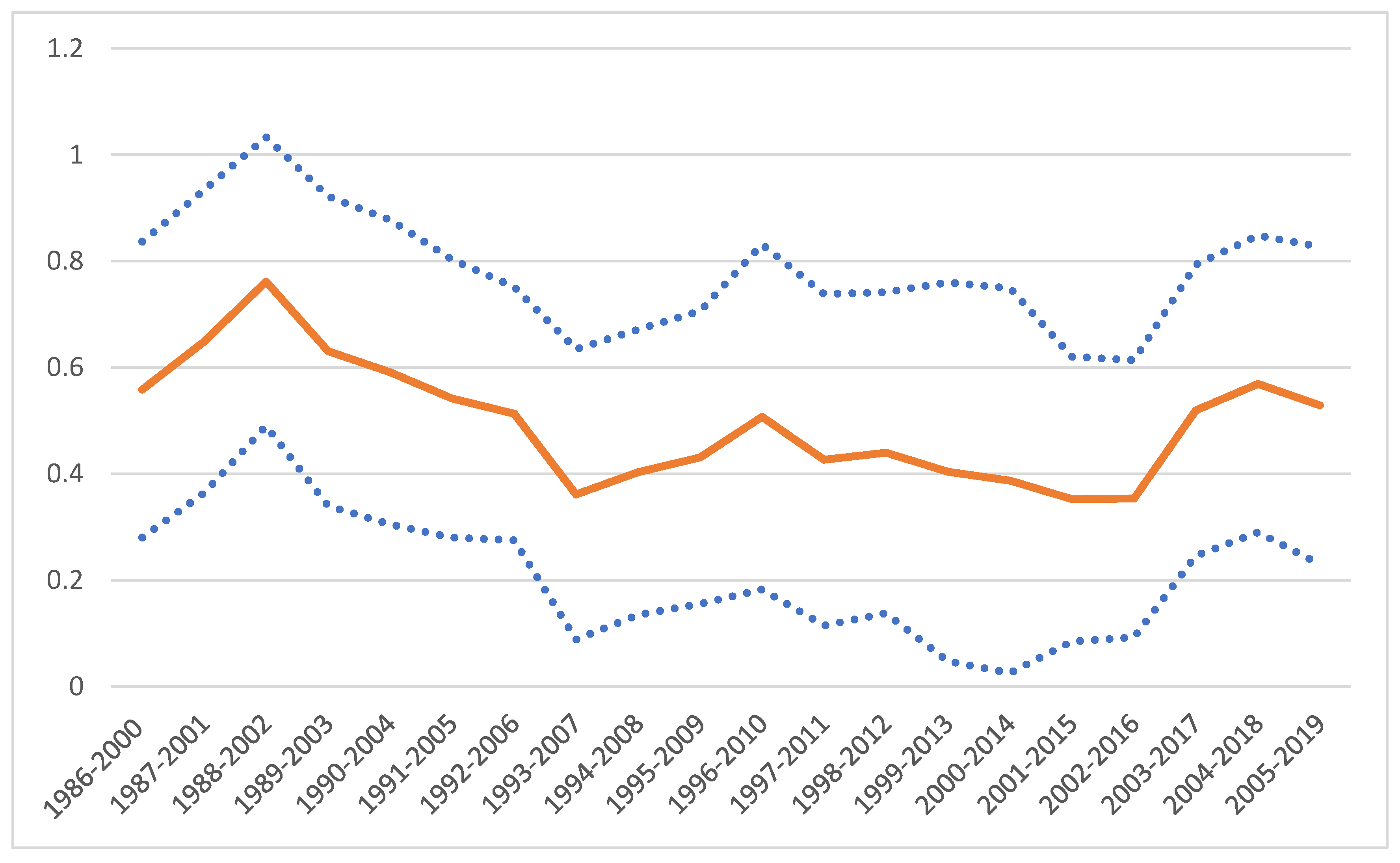
Span	GDP	Price
1986–2000	0.56 ****	−0.06
	[0.28 0.84]	[−0.23 0.12]
1987–2001	0.65 ****	−0.1
	[0.36 0.93]	[−0.26 0.06]
1988–2002	0.76 ****	−0.1
	[0.49 1.03]	[−0.23 0.04]
1989–2003	0.63 ****	−0.02
	[0.34 0.92]	[−0.14 0.10]
1990–2004	0.59 ****	−0.03
	[0.30 0.88]	[−0.13 0.08]
1991–2005	0.54 ****	−0.09 *
	[0.28 0.80]	[−0.20 0.02]
1992–2006	0.51 ****	−0.15 ***
	[0.28 0.75]	[−0.24 −0.05]
1993–2007	0.36 **	−0.19 ****
	[0.09 0.63]	[−0.28 −0.11]
1994–2008	0.40 ***	−0.16 ***
	[0.13 0.67]	[−0.27 −0.04]
1995–2009	0.43 ***	−0.19 ***
	[0.16 0.71]	[−0.30 −0.07]
1996–2010	0.51 ***	−0.16***
	[0.18 0.83]	[−0.26 −0.05]
1997–2011	0.43 ***	−0.15 **
	[0.11 0.74]	[−0.28 −0.02]
1998–2012	0.44 ***	−0.13 *
	[0.14 0.74]	[−0.27 0.00]
1999–2013	0.40 **	−0.14 **
	[0.05 0.76]	[−0.27 −0.01]
2000–2014	0.39 **	−0.13 **
	[0.03 0.75]	[−0.24 −0.02]
2001–2015	0.35 **	−0.12 **
	[0.08 0.62]	[−0.22 −0.02]
2002–2016	0.35 ***	−0.07 *
	[0.09 0.61]	[−0.16 0.01]
2003–2017	0.52 ****	−0.06
	[0.25 0.79]	[−0.14 0.02]
2004–2018	0.57 ****	−0.06
	[0.29 0.85]	[−0.15 0.04]
2005–2019	0.53 ***	−0.06
	[0.23 0.83]	[−0.16 0.04]

Notes: ****, ***, **, * indicate statistical significance at the 0.001, 0.01, 0.05, and 0.1 levels, respectively. 95% confidence intervals in brackets.

displays the 15-year rolling regressions for a static demand model (Appendix A Figure A1 shows the GDP elasticity results in graphic form). These regressions do not suggest a systematic change in the GDP elasticity. The GDP elasticity is always statistically significant, and for only one regression is unity within the confidence interval. For the time span non-overlapping regressions, e.g., the first four and last three time spans, the elasticities are similar in magnitude, and all have confidence intervals that contain all seven GDP coefficients. The average GDP elasticity for the 20 regressions is 0.5, which is contained within the confidence interval of each of those 20 regressions. While there is some variation among the 20 regressions, very few estimation pairs have confidence intervals that do not overlap. In other words, there are very few GDP elasticity estimations that would be statistically significantly different from one another, and those few do not occur in any systematic pattern or over nearby/consecutive time spans.

Not only is the average GDP elasticity 0.5, nearly all the individual time span estimations are below 0.7, the number found in the previously discussed recent work; however, 0.7 is within the confidence intervals of all but four regressions. Furthermore, the results in Table 3 come from a static model, not a dynamic one as used in [14]. In addition, a more recent (i.e., from the 1990s onward) post-energy crises GDP elasticity of 0.6–0.5 would be consistent with a time-invariant estimation that considered data from 1960–1975—when the elasticity may have been closer to one—and produced an elasticity of 0.7 on average. (For example, for the 37-country OECD panel considered by [14], only 17 countries had data for 1960–1977; 11 countries’ data began in the 1970s (most often in 1978), and another 9 had data that began in the 1990s.)

Further still, these regressions could support the Gao et al. [16] finding that the GDP elasticity has dropped below 0.7. Indeed, total final energy consumption per capita peaked in many OECD countries around the time of the Great Recession (e.g., 2008). While in the following decade, energy consumption did not fully rebound to its previous level, neither did consumption typically continue to decline. Hence, a slight drop in the GDP elasticity of economy-wide energy consumption from that point in time is possible/plausible. Altogether, the results presented in Table 3 point to a more-or-less stable GDP elasticity from the 1990s onward.

Most of the results presented in Table 2 and Table 3 are in concert with previous work. The most notable exceptions to this consistency are (i) the below unity GDP elasticity for 1970 and 1980 estimated by [13]; and (ii) the stable and below unity GDP elasticity over 1960–1985 estimated by [16] for their all-countries panel. (It is important to note that the very low GDP elasticity estimated by [23] runs counter to all previous work of which we are aware (e.g., [9,10,13,14,16,19,24]).) While the reasons for these two such exceptions are not obvious, [13] considers only two years of data (i.e., simple cross-sections) and combines developed and developing countries, for which the GDP elasticities may be different at those times (e.g., see [10]). In addition, the analysis of [13] does not consider energy prices. As mentioned before, the methods of [16] appear to perform best when the number of cross sections is large. When [16] analyzed an OECD panel, their results post-late-1970s are consistent with the argument made here: the GDP elasticity fell from over one (pre-energy crises) to under one (post-energy crises), and then from around 1990–2016, the elasticity fell only slightly. However, over the period 1960–1977—when their analysis included only 17 countries, even fewer than the panel analyzed here—their results do not lend themselves to a clear explanation. From 1960 to around 1968 the GDP elasticity fell from 1.6 to around 0.5, from which it increased to around 1.2 in around 1977. (Results from semi-parametric methods can display beginning- and end-of-sample effects).

5. Conclusions

In sum, given the findings of [19,24] and the regressions displayed in Table 2 here: (i) the GDP elasticity for economy-wide energy demand was around unity for OECD countries prior to the first energy crisis; and (ii) the reactions to the extreme oil price experiences that occurred over 1975–1985 led to a substantially lower GDP elasticity for economy-wide energy in OECD countries. Again, examples of these reactions were appliance efficiency standards and consumer preference toward energy savings. Such a determination extends to the GDP elasticity the asymmetry literature’s judgements regarding the price elasticity—viz., price elasticities of demand became smaller in absolute terms as the multiple responses to the price spike had a permanent effect on energy demand. Further, we conclude that, given the results of [16] and the regressions shown in Table 3 here, the GDP elasticity for economy-wide energy demand in OECD countries is around 0.6–0.5 and has been fairly stable at that level since the end of the second energy crisis, i.e., since about 1986. While the new evidence of post-crises GDP elasticity constancy may not be overwhelmingly convincing, we believe that when combined with the earlier results (i.e., [10,13,15,16,19,24]), the new evidence of a lower elasticity post-crises compared to pre-crises, and the arguments as to why elasticities change, this paper has made a definitive case.

The implications of the first conclusion—that the GDP elasticity declined in a step-like manner rather than in a smooth, continuous manner—are that lessening the relationship between energy consumption and GDP occurs through a concerted effort rather than as part of the development or dematerialization process. The implication of the second conclusion—that since the impact of the responses to the energy crises, the GDP elasticity has been essentially constant despite further improvements in technology/energy efficiency—is that the economy-wide rebound effect is close to 100% (in the absence of concerted policy efforts) as some recent reviews [33,34] have argued.

Hence, a key question/issue to address in future work given the current concern over global climatic change is whether the substantial decrease in the GDP elasticity of energy consumption that resulted from reactions to the energy crises can be further replicated, or whether the fairly constant GDP elasticity of energy consumption over the past 35 years suggests that the decoupling of GDP and energy after the energy crises represented picking off all the low hanging fruit. If so, climate mitigation may have to lean on the decarbonization of energy supply.

References

- Dargay, J.M. The irreversible effects of high oil prices: Empirical evidence for the demand for motor fuels in France, Germany and the UK. In Energy Demand: Evidence and Expectations; Hawdon, D., Ed.; Surrey University Press: Guildford, UK, 1992; pp. 165–182. [Google Scholar]
- Walker, I.O.; Wirl, F. Irreversible price-induced efficiency improvements: Theory and empirical application to road transportation. Energy J. 1993, 14, 183–205. [Google Scholar] [CrossRef]
- Dargay, J.M.; Gately, D. The imperfect price-reversibility of non-transport oil demand in the OECD. Energy Econ. 1995, 17, 59–71. [Google Scholar] [CrossRef]
- Dargay, J.M.; Gately, D. The demand for transportation fuels: Imperfect price reversibility? Transp. Res. B 1997, 31, 71–82. [Google Scholar] [CrossRef]
- Gately, D.; Huntington, H.G. The asymmetric effects of changes in price and income on energy and oil demand. Energy J. 2002, 23, 19–55. [Google Scholar] [CrossRef]
- Ryan, D.; Plourde, A. Smaller and smaller? The price responsiveness of non-transport oil demand. Q. Rev. Econ. Financ. 2002, 42, 285–317. [Google Scholar] [CrossRef]
- Huntington, H.G. Oil demand and technical progress . Appl. Econ. Lett. 2010, 17, 1747–1751. [Google Scholar] [CrossRef]
- Goldemberg, J. Leapfrog energy technologies. Energy Policy 1998, 2, 729–741. [Google Scholar]
- Van Benthem, A. Energy leapfrogging. J. Assoc. Environ. Resour. Econ. 2015, 2, 93–132. [Google Scholar] [CrossRef]
- Liddle, B.; Huntington, H. There’s Technology Improvement, but is there Economy-wide Energy Leap-Frogging? A Country Panel Analysis. World Dev. 2021, 140, 105259. [Google Scholar] [CrossRef]
- Galli, R. The relationship between energy and income levels: Forecasting long term energy demand in Asian emerging countries. Energy J. 1998, 19, 85–105. [Google Scholar] [CrossRef]
- Medlock, K.; Soligo, R. Economic development and end-use energy demand. Energy J. 2001, 22, 77–105. [Google Scholar] [CrossRef]
- Csereklyei, Z.; Rubio Varas, M.; Stern, D. Energy and economic growth: The stylized facts. Energy J. 2016, 37, 223–255. [Google Scholar] [CrossRef]
- Liddle, B.; Huntington, H. Revisiting the income elasticity of energy consumption: A heterogeneous, common factor, dynamic OECD & non-OECD country panel analysis. Energy J. 2020, 41, 207–229. [Google Scholar] [CrossRef]
- Liddle, B.; Smyth, R.; Zhang, X. Time-varying income and price elasticities for energy demand: Evidence from a middle-income panel. Energy Econ. 2020, 86, 104681. [Google Scholar] [CrossRef]
- Gao, J.; Peng, B.; Smyth, R. On income and price elasticities for energy demand: A panel data study. Energy Econ. 2021, 96, 105168. [Google Scholar] [CrossRef]
- Fouquau, J.; Destais, G.; Hurlin, C. Energy demand models: A threshold panel specification of the ‘Kuznets curve’. Appl. Econ. Lett. 2009, 16, 1241–1244. [Google Scholar] [CrossRef]
- Pablo-Romero, M.; Sanchez-Braza, A. Residential Energy Environmental Kuznets Curve in the EU-28. Energy 2017, 125, 44–54. [Google Scholar] [CrossRef]
- Brookes, L.G. More on the output elasticity of energy consumption. J. Ind. Econ. 1972, 21, 83–92. [Google Scholar] [CrossRef]
- Chang, Y.; Choi, Y.; Kim, C.; Miller, J.; Park, J. Disentangling temporal patterns in elasticities: A functional coefficient panel analysis of electricity demand. Energy Econ. 2016, 60, 232–243. [Google Scholar] [CrossRef]
- Bai, J. Panel data models with interactive fixed effects. Econometrica 2009, 77, 1229–1279. [Google Scholar] [CrossRef]
- Pesaran, M.H. Estimation and inference in large heterogeneous panels with a multifactor error structure. Econometrica 2006, 74, 967–1012. [Google Scholar] [CrossRef]
- Chang, Y.; Choi, Y.; Kim, C.; Miller, I.; Park, J. Forecasting regional long-run energy demand: A functional coefficient panel approach. Energy Econ. 2021, 96, 105117. [Google Scholar] [CrossRef]
- Adams, F.G.; Miovic, P. On relative fuel efficiency and the output elasticity of energy consumption in Western Europe. J. Ind. Econ. 1968, 17, 41–56. [Google Scholar] [CrossRef]
- Hamilton, L. How robust is robust regression? Stata Tech. Bull. 1991, 2, 21–26. [Google Scholar]
- Pesaran, M.H.T. Yamagata. Testing slope homogeneity in large panels. J. Econom. 2008, 142, 50–93. [Google Scholar] [CrossRef]
- Chudik, A.; Pesaran, M. Common correlated effects estimation of heterogeneous dynamic panel data models with weakly exogenous regressions. J. Econom. 2015, 188, 393–420. [Google Scholar] [CrossRef]
- Nickell, S. Biases in dynamic models with fixed effects. Econometrica 1981, 49, 1417–1426. [Google Scholar] [CrossRef]
- Beck, N.; Katz, J. Modeling dynamics in time-series—cross-section political economy data. Annu. Rev. Polit. Sci. 2011, 14, 331–352. [Google Scholar] [CrossRef]
- Judson, R.; Owen, A. Estimating dynamic panel data models: A guide for macroeconomists. Econ. Lett. 1999, 65, 9–15. [Google Scholar] [CrossRef]
- Westerlund, J.; Perova, Y.; Norkute, M. CCE in fixed-T panels. J. Appl. Econom. 2019, 34, 746–761. [Google Scholar] [CrossRef]
- Pesaran, H.; Shin, Y.; Smith, R. Pooled mean group estimation of dynamic heterogeneous panels. J. Am. Stat. Assoc. 1999, 94, 621–634. [Google Scholar] [CrossRef]
- Stern, D. How large is the economy-wide rebound effect? Energy Policy 2020, 147, 111870. [Google Scholar] [CrossRef]
- Brockway, P.; Sorrell, S.; Semieniuk, G.; Kuperus Heun, M.; Court, V. Energy efficiency and economy-wide rebound effects: A review of the evidence and its implications. Renew. Sustain. Energy Rev. 2021, 141, 110781. [Google Scholar] [CrossRef]