Data Reduction and Reconstruction of Wind Turbine Wake Employing Data Driven Approaches

Abstract

Data driven approaches are utilized for optimal sensor placement as well as for velocity prediction of wind turbine wakes. In this work, several methods are investigated for suitability in the clustering analysis and for predicting the time history of the flow field. The studies start by applying a proper orthogonal decomposition (POD) technique to extract the dynamics of the flow. This is followed by evaluations of different hyperparameters of the clustering and machine learning algorithms as well as their impacts on the prediction accuracy. Two test cases are considered: (1) the wake of a cylinder and (2) the wake of a rotating wind turbine rotor exposed to complex flow conditions. The training and test data for both cases are obtained from high fidelity CFD approaches. The studies reveal that the combination of a classification-based machine learning algorithm for optimal sensor placement and Bi-LSTM is sufficient for predicting periodic signals, but a more advanced technique is required for the highly complex data of the turbine near wake. This is done by exploiting the dynamics of the wake from the set of POD modes for flow field reconstruction. A satisfactory accuracy is achieved for an appropriately chosen prediction horizon of the Bi-LSTM networks. The obtained results show that data-driven approaches for wind turbine wake prediction can offer an alternative to conventional prediction approaches.

1. Introduction

Predicting wind turbine wakes is an important topic in wind farm design and operation. It is well known that the inflow conditions of wind turbines in the wind farm are highly influenced by the wake of neighboring turbines. This can result in a significant power loss and increased transient loads. Numerous analytical, numerical and experimental investigations were conducted in the past to understand the wakes of wind turbines [1,2,3,4,5,6,7,8,9,10,11]. These models can vary in complexity and fidelity levels.

Capturing the whole physics of wind turbine near wake by means of experimental approach is a challenging task due to the highly unsteady nature of the flow. Numerous studies were focused on laboratory scale investigations with controlled flow conditions [4,5,6]. In contrast, the situation is much more complex in reality, including the effects of wake interaction, controller activities and atmospheric flow conditions. These aspects make it difficult and expensive to capture the whole dynamics of the near wake. Although complex wake structures can be captured by high fidelity computational approaches, as done in [7,8,9,10,12], they are not suitable for real-time control applications [13]. In contrast, low order methods are well established in industry because they are cheap and computationally efficient, but the accuracy depends strongly upon the underlying assumptions and in certain cases they require a number of empirical corrections [10,14,15].

In recent years, the popularity of machine learning based techniques for reduced order modeling of physical systems has increased greatly. The same is also true for the data reduction techniques for representing the whole system, well known as the optimal sensor placement. For a high-dimensional system, the cluster-based reduced-order modeling (CROM) technique proposed by Kaiser et al. [16] enables the derivation of a low-order kinematic description in the state space and a corresponding probabilistic dynamic model. A powerful technique for estimating a limited number of optimally placed sensors was derived by Brunton et al. [17]. The sparse sensor placement optimization for classification (SSPOC) enables an accurate prediction in classification task. Furthermore, sparse sensor placement optimization for reconstruction (SSPOR) proposed by Manohar et al. [18] delivers a useful approach for estimating a small set of sensors which reconstruct a signal with most possible accuracy.

The great success of machine learning in the recent years is indivisible with huge improvements of artificial neural networks (ANNs), including recurrent neural networks (RNNs). The bidirectional long short-term memory (Bi-LSTM) networks are the prime example of a powerful RNN type since they include all available sequential information during computation [19]. Data-driven approaches enable alternative methodologies for predicting the wind turbine wakes in real-time applications. Ali et al. [13] demonstrated a procedure applied to large eddy simulation (LES) results of a wind turbine by applying the CROM and SSPOC for sensors placement estimation and Bi-LSTM networks for wake prediction. Despite that, these studies were focused on the far wake prediction. Iungo et al. [20] also attempted to employ data driven technique for wake prediction based on CFD data as reference, but no spare sensor placement technique was adopted, requiring it to use the entire flow snapshots. Other studies were found to focus on the SCADA data [21,22,23] without providing an estimate on the flow field predictions. Recently, D’Agostino et al. [24,25] also attempted to use cluster analysis and time series prediction for different applications, showing the potential of data driven approaches.

The Bi-LSTM method is deemed suitable for complex timeseries prediction, as already observed in several works. It has been demonstrated in the field of speech recognition that Bi-LSTM is advantageous for processing the sequential data. For example, Graves and Schmidhuber [26] have shown that Bi-LSTM outperformed unidirectional LSTM, bidirectional RNN, unidirectional RNN and MLPs. Further studies included different applications in timeseries predictions [27,28,29,30]. Huang et al. [27] proposed a TSF-CGANs algorithm for photovoltaic power forecasting, in which Bi-LSTM was adopted. They chose Bi-LSTM since it showed the best suitability compared to LSTM, RNN, BP, SVM and Persistence models. Vo et al. [28] predicted the brent oil price, comparing the performance of LSTM, a combination of CNN and LSTM, a combination of CNN and Bi-LSTM and a newly proposed model, the so called BOP-BL model, which is similar to the stacked Bi-LSTM architecture adopted in this work. Based on the studies, they recommend Bi-LSTM based models for predicting the timeseries data. Le et al. [29] compared the performance of linear regression, LSTM, CNN-LSTM and CNN-Bi-LSTM for predicting the electric energy consumption. The CNN-Bi-LSTM model outperformed the other state-of-the-art models, and this model is highly similar to the approach will be used in the present work, i.e., the feature extraction in [29] was provided by the CNN module, whereas in this work the equivalent feature extraction step will be realized through optimal sensor placement for estimation of the most informative spatial locations in the snapshot data. Based on all these past studies, it becomes reasonable to adopt the Bi-LSTM method as the major workforce of the present investigations.

It can be seen that there are still clear gaps in exploiting the potential of data driven techniques for the near wake predictions of wind turbines. This paper is aimed at filling these gaps and providing an alternative method for predicting the wind turbine near wake using data driven approaches. The capability of several methods to predict the wake will be investigated in this paper. The studies will be carried out for two different cases with varying complexity levels: (1) the wake of a cylinder and (2) the wake of a rotating turbine exposed to complex flow conditions. Results from high fidelity computational fluid dynamics (CFD) computations are used for defining the training and test data for both cases. Initially, a method proposed by Ali et al. [13] will be followed. Since this method was only tested on the far wake of wind turbine which contained only large scale fluctuations, this will be proven challenging. To test this attempt, the cylinder case will be contaminated with the initial transient phase having only a limited amount of learning datasets. This is intended because the data of the wind turbine case as the core of the studies is also very limited. Based on the initial cylinder case study, various different approaches will be adopted for the wind turbine case, ranging from the clustering method using k-means, Gaussian mixture model, hierarchical agglomerative clustering to reconstruction (based on regression) approaches.

A proper orthogonal decomposition (POD) technique will be applied for the sake of data reduction, followed by a k-means clustering in the POD subspace. A linked approach between CROM and SSPOC will be applied for estimating the small set of optimally placed sensors. In addition to that, the usage of SSPOR for optimum sensor placement is further tested to determine the performance of various modeling strategies. By employing aforementioned machine learning algorithms, most informative sensor locations in the near wake are to be identified and will be utilized for a further prediction task by means of the Bi-LSTM networks. This will allow timeseries predictions of the flow field at sensor locations to be made. Different settings of the employed training, validation and test data as well as different lengths of input and output timeseries will be investigated. These include the studies on the optimal number of layers and number of units per layer of the Bi-LSTM networks by conducting a grid search. The studies will present strategies for appropriately perform a data reduction technique and for predicting the velocity measurement timeseries of the near wake of wind turbine exposed to realistic flow conditions.

This paper is organized as following. Section 2 presents detailed description of the chosen approaches and the employed datasets. The results will be discussed in Section 3, containing two major parts for the wake of cylinder in Section 3.1 and for the wake of wind turbine in Section 3.2. All the results will be summarized and concluded in Section 4.

2. Methodology

2.1. High Fidelity CFD Data

2.1.1. CFD Data for Cylinder Computations

The results of a two-dimensional direct numerical simulation (DNS) of a flow around a cylinder are used here, downloaded from the web page of the computer graphics laboratory of the ETH Zürich, from [31]. This dataset was originally used in Günther et al. [32]. The flow domain consists of a channel with two solid walls, which are considered with a slip boundary condition. From the left, the fluid was injected. Downstream, nearby the inflow area, a cylinder was placed. For the solution of this 2D viscous flow, the Gerris flow solver [33], was utilized. For the simulation, an unstructured grid was used with adaptive discretization regarding the vorticity. To obtain the solution for a regular grid, a subsequent resampling was performed. Further details are listed in 

Table 1. Numerical setting (all variables are dimensionless), from [31].

Physical Quantity	Value
regular grid resolution (X × Y × T)	640 × 80 × 1501
simulation domain	[−0.5, 7.5] × [−0.5, 0.5] × [0, 15]
Reynolds number	160
kinematic viscosity	0.00078125
obstacle at (0, 0) with radius	0.0625

.

The dataset comprises 1501 snapshots of the flow field, which are referred by a temporal index $i_t$. They are arranged in chronological order with $i_t=0\dots 1500$. Each snapshot consists of the velocity components in x- and y-direction given for each grid point. The x-axis direction corresponds to the downstream flow direction, the y-axis is perpendicular to it. Figure 1 illustrates the wake characteristics downstream of the cylinder. The dataset can be divided into the transient flow initialization phase and a following periodic quasi steady state.

2.1.2. CFD Data for Wind Turbine Computations

For the main investigations in this work, a dataset is considered describing the three-dimensional fully turbulent flow around a horizontal axis wind turbine and the near-wake [10]. The dataset consists of 2250 snapshots of the velocity field. They are equally spaced in time, with a time step between two snapshots of $\mathsf{\Delta }t=4.115\times {10}^{-2}$ s. Consistent to the cylinder flow dataset, in the context of this work the snapshots are referred by their corresponding temporal index $i_t=0\dots 2249$. Each snapshot provides the velocity vector at each grid point on the x-z-plane for $y=0\mathrm{m}$. The velocity vector contains the velocity components in x-, y- and z-direction u, v and w, respectively. The uniform grid in which the velocity field is stored consists of $n_x=581$ and $n_z=251$ grid points in x- and z-direction, respectively.

In the studies, the NM-80 (DanAero) wind turbine was adopted. This turbine has a rated power of 2.3 MW with a rotor diameter of 80 m. This turbine is also thoroughly investigated within the IEA Wind Task 29 Phase IV, commonly referred as MEXNEXT project [34], and now within the IEA Wind Task 47, commonly referred as TURBINIA project. The turbine was measured during the DanAero measurement campaign between 2007–2010 in cooperation between the Technical University of Denmark (DTU) and the industrial partners Vestas, Siemens LM and DONG Energy. The NM-80 turbine measurement was located in the Tjaereborg wind farm.

The CFD computations were done by employing the FLOWer code [35] with the advanced DDES (delayed–detached eddy simulation) technique implemented at IAG [36]. The adopted numerical scheme was based on a finite-volume formulation implemented on block-structured grids. The spatial discretization used a second order central discretization with artificial damping according to Jameson-Schmidt-Turkel (JST) method [37] in the near wall area and the 5th order weighted essentially non-oscillatory scheme WENO for resolving the turbulent eddies in the wake [38]. The time integration was accomplished by adopting an explicit multistage scheme. The calculations were done by utilizing the total number of cells as high as 132 million to properly resolve relevant physical flow characteristics. The turbulent inflow was generated by Mann turbulence box, injected in all directions as a momentum source term [39] at $x=-320\mathrm{m}$ upstream of the rotor. The simulation results were validated with experimental data [10], and good agreements were obtained. Figure 2 illustrates the wake characteristics downstream of the turbine. It can bee seen that the flow is far more complex than the cylinder case in Figure 1.

2.2. Sensor Placement

For the datasets described in Section 2.1.1 and Section 2.1.2, a set of optimally placed sensors was estimated. Therefore, in the following, two different approaches are reported: (1) classification based approach in Section 2.2.1 and (2) reconstruction based approach in Section 2.2.2. Firstly, a similar approach as performed by Ali et al. [13] which utilizes the CROM (cluster-based reduced-order modelling) [16] in combination with SSPOC (sparse sensor placement optimization for classification) [17] was adopted. Furthermore, for the wind turbine case, sparse sensor placement optimization for reconstruction (SSPOR) proposed by Manohar et al. [18] was applied as a second distinct technique for optimal sensor placement based on data reconstruction.

2.2.1. Classification Based Approach

A linked approach of CROM in combination with SSPOC was adopted for both cylinder and wind turbine cases. In detail, a proper orthogonal decomposition (POD) was conducted with a subsequent clustering analysis by means of the k-means algorithm. The step of data reduction by means of the POD decreases the computational effort required for k-means clustering, since the snapshots are represented in the low-dimensional POD subspace, which reduces the memory requirements significantly. Note that the distance-based metric of the k-means algorithm is more effective for low-dimensional data [40]. Optimally, the cluster analysis delivers an appropriate partition of the snapshot data in the state space. Furthermore, each snapshot is labeled with one certain cluster label, which is necessary for application of SSPOC.

Application of POD in this paper is primarily for dimension reduction, for a more efficient application of the k-means clustering. In case of an orthonormal basis, the Euclidean distance of the snapshots in the state space is also valid in the mode coefficient subspace [16]. Hence, application of the k-means clustering in the mode coefficient subspace is significantly more efficient, since the dimensionality of the POD subspace is significantly smaller compared to the state space of the snapshots. Physical interpretation and investigation of the achieved POD modes will be conducted as an additional secondary task. Since the modes obtained from the other method, e.g., dynamic mode decomposition (DMD), are not orthogonal in general, DMD was considered less suitable for exploiting this approximation. Furthermore, in the context of SSPOR, Manohar et al. [18] suggested that utilization of non-normal modes for sensor selection is still accompanied by some problems and is subject of ongoing research.

In the preprocessing step, the raw snapshot data was prepared for suitable treatment by POD and clustering algorithms. A single snapshot contains the velocity components in x-, y- and z-direction u, v and w, respectively, for each grid point. For each velocity component separately, the grid point data was rearranged row by row, i.e., after transposing each row they were all stacked vertically in a column vector. The final snapshot column vector was obtained by vertically stacking the vectors of each velocity component. Hence, each snapshot of the raw dataset was rearranged in a column vector. In 1 to 2, the procedure for rearrangement is illustrated. Variables $n_x$ and $n_z$ denote the number of grid points in x- and z-directions, respectively.

$${\left[\begin{array}{ccc}{\varphi }_{11}^i& \cdots & {\varphi }_{n_{x}1}^i\\ ⋮& \ddots & ⋮\\ {\varphi }_{1n_z}^i& \cdots & {\varphi }_{n_x{n}_z}^i\end{array}\right]}_{i_t}\to {\left[\begin{array}{c}\left(\begin{array}{c}{\varphi }_{11}^i\\ ⋮\\ {\varphi }_{n_{x}1}^i\end{array}\right)\\ ⋮\\ \left(\begin{array}{c}{\varphi }_{1n_z}^i\\ ⋮\\ {\varphi }_{n_x{n}_z}^i\end{array}\right)\end{array}\right]}_{i_t}\mathrm{with}i\in 1,2,3;{\varphi }^1=u,{\varphi }^2=v,{\varphi }^3=w$$

(1)

$${\left[\begin{array}{c}{u}_{11}\\ ⋮\\ u_{n_x{n}_z}\end{array}\right]}_{i_t},{\left[\begin{array}{c}{v}_{11}\\ ⋮\\ v_{n_x{n}_z}\end{array}\right]}_{i_t},{\left[\begin{array}{c}{w}_{11}\\ ⋮\\ w_{n_x{n}_z}\end{array}\right]}_{i_t}\to {\left[\begin{array}{c}\left(\begin{array}{c}{u}_{11}\\ ⋮\\ u_{n_x{n}_z}\end{array}\right)\left(\begin{array}{c}{v}_{11}\\ ⋮\\ v_{n_x{n}_z}\end{array}\right)\left(\begin{array}{c}{w}_{11}\\ ⋮\\ w_{n_x{n}_z}\end{array}\right)\end{array}\right]}_{i_t}^T=\mathit{q}\left(i_t\right)$$

(2)

After estimating the temporal mean vector of the m snapshots

$$\overline{\mathit{q}}=\frac{1}{m}\sum _{i=0}^{m-1}\mathit{q}(i_t=i),$$

(3)

the fluctuating component of each snapshot was obtained by

$$\mathit{x}\left(i_t\right)=\mathit{q}\left(i_t\right)-\overline{\mathit{q}}\mathrm{with}{i}_t\in [0,m-1]\subseteq \mathbb{N}.$$

(4)

All fluctuation vectors were collected in

$$\mathit{X}=\left[\mathit{x}\right(0\left)\mathit{x}\right(1)\cdots \mathit{x}(m-1\left)\right].$$

(5)

After estimating $\mathit{X}$, by means of the modred library [41], the POD was computed. The number of POD modes to estimate was set to the maximum possible value, since it is always $n_{POD}\le m-1$[16]. By applying the method of snapshots [42], the desired POD modes ${\mathbf{\Phi }}_i$, the corresponding eigenvalues ${\lambda }_i$ and the vectors containing the temporal POD coefficients $\mathit{a}\left(i_t\right)$ were obtained.

The subsequent clustering analysis of the snapshots was performed in the POD subspace, in which each snapshot $\mathit{q}\left(i_t\right)\in {\mathbb{R}}^{2n_x{n}_z}$ is represented by $\mathit{a}\left(i_t\right)\in {\mathbb{R}}^{m-1}$. For better clustering performance the input data was normalized, i.e., transformation of the data to the range $[0,1]\subseteq \mathbb{R}$, by means of the MinMaxScaler provided by the Python package scikit-learn [43]. The k-means clustering was performed for different values of k, since the appropriate number of clusters k was unknown beforehand. By means of the elbow method and silhouettes, an appropriate k should be chosen.

Instead of random seeding in case of the standard k-means algorithm, k-means++ is applied here for better performance. Finally, one obtains the centroids ${\mathit{c}}_1,\dots ,{\mathit{c}}_k$, the snapshot labels $\mathit{y}=[y_1,\dots ,y_m]$ and the inertia I (sum of squared distance of snapshots to its corresponding centroids).

An eigenvalue ${\lambda }_j$ can be considered as a measure of the contributed portion of a POD mode ${\mathbf{\Phi }}_j$ to the total fluctuation kinetic energy. To capture the portion ${ϵ}_{POD}$ of kinetic fluctuating energy, the number r of minimum required first POD modes can be estimated with:

$$r=\underset{r^{\prime }}{arg\; min}\left\{r^{\prime }\right\},\mathrm{subject}\mathrm{to}{ϵ}_{POD}\le \frac{{\sum }_{j=1}^{r^{\prime }}{\lambda }_j}{{\sum }_{j=1}^{n_{POD}}{\lambda }_j},$$

(6)

with $n_{POD}$ denoting the total number of POD modes. To investigate truncation of POD modes, the four setups listed in 

Table 2. Different settings for k-means clustering for the wind turbine case.

Setup	r	${\mathit{k}}_{\mathbf{max}}$	${\mathit{ϵ}}_{\mathbf{POD}}$ in %
1	2249	300	100
2	11	20	45
3	19	50	59
4	27	75	69

were considered for k-means clustering for the wind turbine case. For the cylinder wake, all available POD modes were considered. In each case, only the first r POD modes were considered to capture the fraction ${ϵ}_{POD}$ of the total fluctuating kinetic energy. The respective $k_{max}$ for each setup is also listed. In case of the cylinder wake dataset, subsequent to the CROM, SSPOC was applied for optimal sensor placement. The dataset was split up into training and test data for model training and error evaluation, respectively. The optimum parameters of the SSPOC model were estimated employing the Bayesian optimization, Gaussian mixture model and hierarchical agglomerative clustering.

2.2.2. Reconstruction Based Approach

For the wind turbine dataset, additionally, a further approach for optimal sensor placement was employed. Sparse sensor placement optimization for reconstruction (SSPOR) proposed by Manohar et al. [18], is a powerful technique to estimate optimally placed sensors tailored on a specific type of signal for a maximum possible signal reconstruction. In this context the python package PySensors [44] was used.

Within the framework of SSPOR, an SVD is conducted and the snapshot data is represented in the POD subspace. It is possible to truncate higher POD modes; hence, they are not used as basis modes. It is assumed that the number of used POD modes compared to the total number of available POD modes has a substantial influence on the accuracy of the flow field reconstruction based on the estimated sensors. This assumption is based on the argumentation that each POD mode captures some portion of the flow dynamics and by truncation of dominant POD modes it is not possible to reconstruct the dominant flow structures. In the following, the conducted investigations regarding the influence of the number of used basis modes on the reconstruction accuracy are described. Firstly, the reconstruction error based on the number of basis modes was considered. Furthermore, the statistical properties of predicted and true signals at some few spatial locations were compared for variation of the number of used basis modes. In all cases the number of sensors was always set equal to the number of basis modes.

The preprocessing step of the snapshot data is always the same. The raw snapshot data was rearranged in column vectors, as already described in Section 2.2.1. According to Equations (1) and (2) for each velocity component the data of a single snapshot was rearranged in a column vector and the distinct vectors were stacked vertically so that finally each snapshot was rearranged in a separate column vector. The snapshot data was split up into a training set ${\mathit{X}}_{train}$ and test set ${\mathit{X}}_{test}$ in the ratio of 3:1, i.e., the first $m_{train}=1688$ snapshots were used for training and the last $m_{test}=562$ snapshots were used for evaluation of the reconstruction error.

a.

Variation of basis modes

For a desired number of basis modes r, by means of SSPOR it is possible to estimate a set of sensors which are optimally placed in the near-wake. With measurements obtained from these sensors, the corresponding flow field can be reconstructed with some error. In the following, the dependency between the reconstruction error and the number of used basis modes r should be investigated. Hence, different values of r within SSPOR are to be applied and the reconstruction error will be evaluated. The number of sensors is always set to $n_s=r$. Hence, the dependency between the reconstruction error and the number of sensors is implicitly considered as well.

For a given r, a SSPOR model is fit to the training data ${\mathit{X}}_{train}$. Thus, a set of optimally placed sensors is obtained. Each snapshot of the test data ${\mathit{X}}_{test}$ is sampled at the estimated sensor locations and a reconstruction of each snapshot is made. The reconstruction error is estimated by comparing the reconstructed and true snapshots of the test data. Here, the root-mean-square error ($RMSE$) over the entire test data is considered:

$$RMSE=\sqrt{\frac{1}{m_{test}}\sum _{i=1}^{m_{test}}\left(\frac{1}{3n_x{n}_z}\sum _{j=1}^{3n_x{n}_z}{(q_{ij,pred}-q_{ij,true})}^2\right)},$$

(7)

with $q_{ij,pred}$ denoting the predicted velocity component at grid point j for the i-th test snapshot and $q_{ij,true}$ representing the corresponding true value. Values of r were chosen from different intervals $[r_{min},r_{max}]\subseteq \mathbb{N}$ with a corresponding step size $s_r$. In 

Table 3. Different setups for variation of basis modes.

Setup	${\mathit{r}}_{\mathit{min}}$	${\mathit{r}}_{\mathit{max}}$	${\mathit{s}}_{\mathit{r}}$
1	1	20	1
2	1	201	10
3	301	1001	100

, the settings are summarized.

b.

Estimation of the smallest possible set of sensors

Since the evaluation of the reconstruction error over the whole flow field is computationally expensive, in the following another approach for evaluating the reconstruction error was applied.The reconstructed and true test data snapshots are evaluated at $n_p=10$ measurement points, according to the following equation:

$$RMSE=\sqrt{\frac{1}{3n_p}\sum _{i=1}^{n_p}\left({(u_{i,pred}-u_{i,true})}^2+{(v_{i,pred}-v_{i,true})}^2+{(w_{i,pred}-w_{i,true})}^2\right)},$$

(8)

where $u_{i,pred}$, $v_{i,pred}$ and $w_{i,pred}$ denote the reconstructed velocity components in x-, y- and z-direction, respectively, for the i-th point. Variables $u_{i,true}$, $v_{i,true}$ and $w_{i,true}$ denote the corresponding true values. The measurement points are arranged vertically at $x=240\mathrm{m}$ with equal spacing in $z=11.5\mathrm{m}\dots 113.5\mathrm{m}$, as depicted in Figure 3.

A final set of sensors as small as possible should be estimated. This is needed to enable real application because each sensor placed in a wind farm increases the installation and maintenance costs in practice. For further evaluation, some additional metrics are considered, which are derived in the following. The mean of the true signal at point $i_p$ is given by

$${\overline{u}}_{i_p,true}=\frac{1}{m_{test}}\sum _{j=1}^{m_{test}}{u}_{j{i}_p,true},$$

(9)

with $u_{j{i}_p,pred}\left(r\right)$ denoting the reconstructed velocity component in x-direction at measurement point $i_p$ for the j-th snapshot of the test data and $u_{j{i}_p,true}\left(r\right)$ being the corresponding true value. The averaged signal mean over all measurement points can be estimated with

$${\overline{u}}_{true}=\frac{1}{n_p}\sum _{i_p=1}^{n_p}{\overline{u}}_{i_p,true}.$$

(10)

Equations (9) and (10) refer to the velocity component in x-direction, but also apply accordingly for the velocity components in y- and z-directions. For the total mean of the true signals, one obtains

$${\overline{x}}_{true}=\frac{1}{3}\sum _{c\in \{u,v,w\}}{\overline{c}}_{true}.$$

(11)

Accordingly, for the variance of the true signals similar formulations can be given:

$$\begin{array}{cc}\hfill s_{i_p,u,true}^2& \hfill =\frac{1}{m_{test}-1}\sum _{j=1}^{m_{test}}{(u_{j{i}_p,true}-{\overline{u}}_{i_p,true})}^2\hfill \end{array}$$

(12)

$$\begin{array}{cc}\hfill s_{u,true}^2& \hfill =\frac{1}{n_p}\sum _{i_p=1}^{n_p}{s}_{i_p,u,true}^2\hfill \end{array}$$

(13)

$$\begin{array}{cc}\hfill s_{true}^2& \hfill =\frac{1}{3}\sum _{c\in \{u,v,w\}}{s}_{c,true}^2.\hfill \end{array}$$

(14)

A similar formulation for the mean and variance of the reconstructed signals can be given. However, the dependency of r must be considered. Hence, for the mean of the reconstructed signals, one obtains

$$\begin{array}{cc}\hfill {\overline{u}}_{i_p,pred}\left(r\right)& \hfill =\frac{1}{m_{test}}\sum _{j=1}^{m_{test}}{u}_{j{i}_p,pred}\left(r\right)\hfill \end{array}$$

(15)

$$\begin{array}{cc}\hfill {\overline{u}}_{pred}\left(r\right)& \hfill =\frac{1}{n_p}\sum _{i_p=1}^{n_p}{\overline{u}}_{i_p,pred}\left(r\right)\hfill \end{array}$$

(16)

$$\begin{array}{cc}\hfill {\overline{x}}_{pred}& \hfill =\frac{1}{3}\sum _{c\in \{u,v,w\}}{\overline{c}}_{pred}\left(r\right).\hfill \end{array}$$

(17)

Finally, for the variance of the reconstructed signals, it is

$$\begin{array}{cc}\hfill s_{i_p,u,pred}^2\left(r\right)& \hfill =\frac{1}{m_{test}-1}\sum _{j=1}^{m_{test}}{(u_{j{i}_p,pred}\left(r\right)-{\overline{u}}_{i_p,pred}\left(r\right))}^2\hfill \end{array}$$

(18)

$$\begin{array}{cc}\hfill s_{u,pred}^2\left(r\right)& \hfill =\frac{1}{n_p}\sum _{i_p=1}^{n_p}{s}_{i_p,u,pred}^2\left(r\right)\hfill \end{array}$$

(19)

$$\begin{array}{cc}\hfill s_{pred}^2\left(r\right)& \hfill =\frac{1}{3}\sum _{c\in \{u,v,w\}}{s}_{c,pred}^2\left(r\right).\hfill \end{array}$$

(20)

For each number of basis modes

$$r\in \{1,6,12,17,23,28,34,39,45,51\},$$

(21)

SSPOR was applied and the reconstructed snapshots were evaluated. In this sense, $n_s=r$ was chosen accordingly.

2.3. Wake Prediction

2.3.1. Wake Prediction for Cylinder Case

For the velocity measurements at the sensor locations, predictions should be made. In this work, a data-driven approach was applied. By means of a bidirectional LSTM (Bi-LSTM) network predictions of ouptut timeseries based on input timeseries should be made. For estimating the appropriate hyperparameters, several grid searches were conducted for different settings. Different sets of training and test data were derived for investigating the learning performance of Bi-LSTM networks regarding periodic flow data, unsteady flow data and a dataset containing both cases.

For the investigations conducted in this work, a stacked Bi-LSTM architecture was chosen as depicted in Figure 4. The input data is processed through $n_l$ Bi-LSTM layers with $n_u$ units per each layer. A single-layer perceptron (SLP) was used as output layer, with each unit connected to each unit of the previous layer. For the units of the output layer, the linear activation function was applied. Meanwhile, the tanh-function was used as activation function for the Bi-LSTM layers and the sigmoid-function was used for the gates of the Bi-LSTM units. The loss was estimated by means of the root-mean-square error (RMSE) between the validation data and its predicted values. For training of the Bi-LSTM network, the Adam algorithm was applied. In this context, the keras [45] submodule of TensorFlow [46] was used.

From the snapshot data at the locations of the estimated optimally placed sensors, the velocity component u (i.e., in x-direction) was extracted for each time step. Hence, for each sensor a timeseries can be derived:

$$(u_{i_s,1},u_{i_s,2},\cdots ,u_{i_s,m})\mathrm{with}{i}_s=1,\cdots ,n_s.$$

(22)

For a suitable treatment with Bi-LSTM, the data was normalized, i.e., the data was transformed into the range $[0,1]\in \mathbb{R}$. The raw timeseries are too long for an appropriate treatment with Bi-LSTM. In practice, timeseries are often used containing not more than 250 to 500 observations [47]. Hence, the timeseries were preprocessed using a sliding window approach. All sensors were considered as input data. In the context of this dataset, predictions should only be made for sensor 4. This was arbitrarily chosen, but each of the remaining sensors is also a possible choice. Hence, the output timeseries contain only data of sensor 4. With the desired number of observations contained in a single input and output series $n_{in}$ and $n_{out}$, respectively, the preprocessing of the raw timeseries applies as followed. The set of derived timeseries

$$S=(S_{in},S_{out})$$

(23)

contains the column vector $S_{in}$ comprising the input timeseries, with its elements defined by

$$S_{in,(i_{ts}+1)}=\left(\left(\begin{array}{c}{u}_{1,i_{ts}}\\ u_{2,i_{ts}}\\ ⋮\\ u_{n_s,i_{ts}}\end{array}\right),\left(\begin{array}{c}{u}_{1,i_{ts}+1}\\ u_{2,i_{ts}+1}\\ ⋮\\ u_{n_s,i_{ts}+1}\end{array}\right),\left(\begin{array}{c}{u}_{1,i_{ts}+2}\\ u_{2,i_{ts}+2}\\ ⋮\\ u_{n_s,i_{ts}+2}\end{array}\right),\cdots ,\left(\begin{array}{c}{u}_{1,i_{ts}+n_{in}-1}\\ u_{2,i_{ts}+n_{in}-1}\\ ⋮\\ u_{n_s,i_{ts}+n_{in}-1}\end{array}\right)\right)\mathrm{with}{i}_{ts}\in [0,n_{ts}-1]\subseteq \mathbb{N}$$

(24)

   and the column vector $S_{out}$ comprising the output timeseries, with its elements defined by

$$S_{out,(i_{ts}+1)}=(u_{4,n_{in}+i_{ts}},u_{4,n_{in}+i_{ts}+1},u_{4,n_{in}+i_{ts}+2},\cdots ,u_{4,n_{in}+i_{ts}+n_{out}-1})\mathrm{with}{i}_{ts}\in [0,n_{ts}-1]\subseteq \mathbb{N},$$

(25)

with $i_{ts}$ denoting the index of a single derived timeseries. One obtains $n_{ts}=m-n_{in}-n_{out}+1$ derived timeseries. $u_{i_s,j}$ denotes the measurement of the velocity in x-direction at sensor $i_s$ for $i_t=j$. The timeseries rearrangement procedure applied the Python function series_to_supervised from Brownlee [48].

It is not necessary to use all of the derived timeseries. It is also possible to specify subintervals of the total considered time range $i_t\in [0,m-1]\subseteq \mathbb{N}$, with m being the number of snapshots,

$$i_{t,train}\in [i_{train,start},i_{train,stop}]\subseteq [0,m-1]\subseteq \mathbb{N}$$

(26)

$$i_{t,test}\in [i_{test,start},i_{test,stop}]\subseteq [0,m-1]\subseteq \mathbb{N},$$

(27)

and use only the corresponding derived timeseries as training and test data. In general, the training data is used for training of a Bi-LSTM network, whereas the learning progress is validated with the test data.

For estimating of optimal hyperparameters for each of the different settings, a grid search was conducted. For a given setting, the search space is spanned by the number of Bi-LSTM layers $n_l$ and the number of units per layer $n_u$

$$n_l\in \{2,5,10,20\}$$

(28)

$$n_u\in \{5,25,50,100,200\}.$$

(29)

The maximum values were limited by the available computing resources. For each point $(n_l,n_u)$ of the parameter grid, a Bi-LSTM network was trained for twenty epochs and with a batch size of thirty-two. RMSE according to 30 was used as the objective for the grid search. The RMSE was estimated in each case after the inverse normalization of the data, i.e., the error validation was performed with data in the original range of values.

$$RMSE=\sqrt{\frac{1}{m_{test}}\sum _{i=1}^{m_{test}}{(u_{4,i,test}-u_{4,i,pred})}^2},$$

(30)

with $m_{test}$ denoting the number of snapshots comprised in the test data, $u_{4,i,test}$ being the true value of sensor 4 at instant $i_t=i$ and $u_{4,i,pred}$ representing the corresponding value predicted by the Bi-LSTM network. Different sets of training and test data and different lengths for input and output series were investigated. In 

Table 4. Different setups for the performance of a grid search.

Setup	Type of Flow	${\mathit{n}}_{\mathit{in}}$	${\mathit{n}}_{\mathit{out}}$	${\mathit{i}}_{\mathit{t},\mathit{train}}$	${\mathit{i}}_{\mathit{t},\mathit{test}}$
1	periodic	50	200	$[751,1125]$	$[1126,1500]$
2	unsteady	50	200	$[0,524]$	$[525,799]$
3	periodic & unsteady	50	200	$\left\{\right[175,474],[901,1200\left]\right\}$	$\left\{\right[475,774],[1201,1500\left]\right\}$
4	periodic & unsteady	25	100	$\left\{\right[175,474],[901,1200\left]\right\}$	$\left\{\right[475,774],[1201,1500\left]\right\}$
5	periodic & unsteady	50	50	$\left\{\right[175,474],[901,1200\left]\right\}$	$\left\{\right[475,774],[1201,1500\left]\right\}$

, the setups are summarized. For each setup, a grid search was conducted as described above.

In the 1st setup, only data with periodic flow conditions was used. The number of observations contained in each input and output timeseries was set to $n_{in}=50$ and $n_{out}=200$, respectively. For the 2nd setup, only data from unsteady flow conditions was used. In the 3rd setup, data for both flow conditions, periodic and unsteady, were considered to investigate the capability of Bi-LSTM network of learning different flow conditions simultaneously. In setup 4, $n_{in}$ and $n_{out}$ are reduced to half the values in the previous setup. To investigate the Bi-LSTM performance for equal lengths of input and output series, it was set $n_{in}=n_{out}=50$ in setup 5. For setups 3, 4 and 5, the same training and test datasets were used.

2.3.2. Wake Prediction for Wind Turbine Case

In this paper, velocity measurements in the near wake of the turbine will be predicted by means of a Bi-LSTM network. Formally, the prediction task can be categorized as univariate multistep timeseries forecasting. In the context of this work, the estimation of optimal sensor locations could be regarded as an equivalent to feature selection in the context of CNN. SSPOR delivers the most informative locations in the flow field. This was done to provide the most appropriate locations to install “physical sensors” in the wake to extract the most useful data. This is primarily useful for wind turbine control purpose. Hence, no further feature selection was conducted. The stacked Bi-LSTM architecture was chosen for a most suitable capturing of the highly nonlinear temporal dependencies within each single sensor signal. The procedures are similar to those of the cylinder flow investigations (see Section 2.3.1).

a.

Spatial sensor data split

The set of sensors was randomly divided into a training set and a test set with a ratio of 3:1. In Figure 5 the sensor division is illustrated. For the training sensors, the entire time range was temporally divided in a training interval and a validation interval, again with a ratio of 3:1. In contrast to the approach described in Section 2.3.1, here the data is split up to training, validation and test data. The training data was used for the training of Bi-LSTM networks, with a simultaneous monitoring of the learning progress by means of the validation data. An obtained Bi-LSTM network was finally tested on the independent test data to evaluate the performance of the model and its ability of generalization. A Bi-LSTM network should be designed which is capable to predict sensor timeseries without explicitly specifying which particular sensor is considered. Hence, the networks were trained with timeseries from all training sensors, but during training it was not specified which sensor belongs to which timeseries. The intent behind this approach was to obtain a Bi-LSTM network which can be applied to an arbitrary test sensor without specifying its location in the flow field.

b.

Standard setup

In the context of this work, a stacked Bi-LSTM architecture was chosen, as depicted in Figure 4. The input timeseries are processed through $n_l$ Bi-LSTM layers with $n_u$ units per each layer. A single-layer perceptron (SLP) was used as output layer, with each unit connected to each unit of the previous layer. For the units of the output layer the linear activation function was applied, as activation function for the Bi-LSTM layers the tanh-function was used and for the gates of the Bi-LSTM units the sigmoid-function was used. The network loss was estimated by means of the mean squared error ($MSE$) between the validation data and its predicted values:

$$MSE=\frac{1}{n_{ts}}\sum _{i=1}^{n_{ts}}\left(\frac{1}{m_{val}}\sum _{j=0}^{m_{val}-1}{(u_{ij,pred}-u_{ij,true})}^2\right).$$

(31)

Here, $n_{ts}$ denotes the number of timeseries used for validation of the Bi-LSTM network, $m_{val}$ denotes the number of observations contained in a single validation timeseries, $u_{ij,true}$ is the j-th timeseries observation of the i-th validation series and $u_{ij,pred}$ is the corresponding prediction. For training of the Bi-LSTM network, the Adam algorithm was applied.

By extracting the measurements of the velocity at each sensor location, one obtains $n_s=20$ raw timeseries. In this work, only the velocity component in x-direction is considered:

$$(u_{i_s,1},u_{i_s,2},\dots ,u_{i_s,m})\mathrm{with}{i}_s=1,\dots ,n_s.$$

(32)

The timeseries were normalized to the range $[0,1]\in \mathbb{R}$ for suitable treatment by Bi-LSTM networks. In practice, for treatment with Bi-LSTM networks, timeseries are often used containing not more than 250 to 500 observations [47]. Since the raw timeseries are too long for an appropriate treatment with Bi-LSTM networks, they were preprocessed using a sliding window approach. With the desired number of observations contained in a single input and output series $n_{in}$ and $n_{out}$, respectively, the preprocessing of the raw timeseries applies as follows. From a raw timeseries of a certain sensor $i_s$, a set of shorter timeseries is derived, which divides into input series and output series for subsequent Bi-LSTM training:

$$S_{i_s}=(S_{i_s,in},S_{i_s,out}).$$

(33)

The column vector $S_{i_s,in}$ comprising the input timeseries is defined by its elements

$$S_{i_s,in,(i_{ts}+1)}=\left(u_{i_s,i_{ts}},u_{i_s,i_{ts}+1},u_{i_s,i_{ts}+2},\cdots ,u_{i_s,i_{ts}+n_{in}-1}\right)\mathrm{with}{i}_{ts}\in [0,n_{ts}-1]\subseteq \mathbb{N}$$

(34)

and the elements of the column vector $S_{i_s,out}$ comprising the output timeseries are defined by

$$S_{i_s,out,(i_{ts}+1)}=(u_{i_s,n_{in}+i_{ts}},u_{i_s,n_{in}+i_{ts}+1},u_{i_s,n_{in}+i_{ts}+2},\cdots ,u_{i_s,n_{in}+i_{ts}+n_{out}-1})\mathrm{with}{i}_{ts}\in [0,n_{ts}-1]\subseteq \mathbb{N}.$$

(35)

   Consequently, one obtains $n_{ts}=m-n_{in}-n_{out}+1$ derived timeseries from the raw timeseries of sensor $i_s$. $u_{i,j}$ denotes the measurement of the velocity in x-direction at sensor i for $i_t=j$. For implementation of the timeseries rearrangement procedure the Python function series_to_supervised from Brownlee [48] was used.

The previous scheme was applied to the raw timeseries of each sensor. In case of the test sensors, the complete time interval $i_t=0\dots 2249$ was considered for derivation of the test data. In case of the training sensors, the above given scheme was applied to the training time interval $i_t=0\dots .1686$ and the validation time interval $i_t=1687\dots 2249$ separately for derivation of the training and validation data, respectively. Finally, each of the derived sets of timeseries for training, validation and test data is split up into input and output data:

$${\mathit{X}}_{train},{\mathit{y}}_{train}$$

(36)

$${\mathit{X}}_{val},{\mathit{y}}_{val}$$

(37)

$${\mathit{X}}_{test},{\mathit{y}}_{test}.$$

(38)

To find an appropriate network configuration, a grid search was conducted. The parameters of the grid search were the number of Bi-LSTM layers and the number of units per each layer. The number of layers was varied between two and eleven, with a step size of three. The number of units per layer was varied between five and fifty, with a step size of fifteen. The choice of this parameter grid was, among other things, influenced by the limitation of computational resources. In 

Table 5. Grid search settings for the spatial sensor data split.

Quantity	Symbol	Value
layers	$n_l$	{2, 5, 8, 11}
units per layer	$n_u$	{5, 20, 35, 50}
epochs	$n_e$	20
batch size	$s_b$	32
input window width	$n_{in}$	150
output window width	$n_{out}$	150

, further settings for the grid search are listed.

With the best setup determined from the grid search, a subsequent training was conducted. However, this time the number of epochs was not fixed to twenty. Instead, an EarlyStopping callback and a ModelCheckpoint callback, provided by keras, were applied to estimate the optimal number of training epochs. By means of the  ModelCheckpoint callback, the validation loss over the number of epochs was monitored and the model with the overall minimum validation loss was saved finally, i.e., the optimally trained Bi-LSTM network was estimated. This prevents overfitting, which is indicated by a decrease of the validation loss over epochs curve until a minimum and a subsequent increase [49].

By means of the EarlyStopping callback, an adaptive training abortion is employed. The validation loss is monitored and the learning process is stopped, if the validation loss does not improve for a specified number of epochs. Here, the epochs limit is set to 25. Finally, for the best hyperparameters estimated from the grid search, a Bi-LSTM network trained with the optimum number of epochs is obtained. Subsequent to the training process, the model is evaluated by making predictions on the test sensor timeseries.

c.

Adjusted window size

By means of the autocorrelation function (ACF) it can be estimated whether a timeseries is autocorrelated or not [50]. To adjust the length of the input and output timeseries in a more reasonable way, here ACF was applied for estimation of appropriate values of $n_{in}$ and $n_{out}$. For calculation of ACF the Python module statsmodels [51] was used. It was assumed that for an appropriate window length, all observations of a certain timeseries are autocorrelated.

By means of ACF for all training sensor timeseries, the maximum number of time steps were estimated for which all observations of one timeseries are correlated. The overall minimum number was chosen in such a way that a correlation between all observations of a certain timeseries derived by the sliding window approach is ensured. As criterion for statistical significance, the 95% confidence interval was used. With the estimated maximum reasonable time lag $l_{max}$, the necessary number of observations $n_{obs}$ in a timeseries is obtained by

$$n_{obs}=l_{max}+1.$$

(39)

Hence, the number of observations contained in a single input and output series $n_{in}$ and $n_{out}$, respectively, was each set to $n_{obs}$. With adjusted settings for $n_{in}$ and $n_{out}$, the grid search described in the previous section was conducted again. The changed parameters are listed in 

Table 6. Grid search settings with adjusted window lengths.

Quantity	Symbol	Value
input window width	$n_{in}$	46
output window width	$n_{out}$	46

.

3. Results and Discussion

3.1. Cylinder Case

3.1.1. Sensor Placement

Considering the first three POD modes in Figure 6, a regular periodic pattern can be observed for the first and second modes, capturing the large scale vortex structures of the Kármán vortex street. The temporal POD coefficients of the first two modes, shown in Figure 7, also reveal a periodic behavior. The envelope begins to increase from $i_t\approx 200$ on and reaches a constant value for the periodic steady state. It can be seen that both coefficients are phase-delayed. A phase shift of around a quarter period time can be estimated. The interaction of POD mode 1 and 2 describes the fluctuation dynamics of the large vortex structures in the wake. This is consistent with observations described by Weiss [52] of a two-dimensional flow around a cylinder at $Re=100$. In contrast to the POD modes described by Weiss, [52], here 18 POD modes are necessary to capture 90% of the fluctuation kinetic energy, not only two. A reason for this discrepancy could be the different Reynolds number (here it is $Re=160$). Another aspect could be the fact, that here a significantly larger flow domain is considered. This could be a reason for more complex POD modes and a wider distribution of the fluctuation kinetic energy among the POD modes. Another reason could be the fact that the dataset is comprised by the transient flow initialization and the followed periodic quasi steady state flow.

POD mode 3 exhibits a significantly different structure, as can be seen in Figure 6. It has some similarity with the time-averaged mean velocity field. It seems like it represents rather a translational portion of the flow than a periodic convection of the vortices. A closer look at the temporal coefficient of the 3rd POD mode in Figure 8 indicates the representation of the transient evolution for the flow initialization.

Following the POD, k-means clustering was applied to the snapshots in the POD subspace. The obtained values of the inertia I for different k are evaluated. The points above the ’elbow’ point indicate that an increase of k leads to no more significant improvement of the inertia. According to the elbow method, for the following investigations it was chosen $k=6$.

In Figure 9, a visualization of the CTM (cluster transition matrix) is given. The yellow squares on the main diagonal show that between most of the snapshots, the assigned cluster remains the same. However, there are some transitions between different clusters, which are indicated by the green and dark purple squares. In Figure 10 an equivalent visualization is shown, however, with the number of transitions from cluster ${\mathcal{C}}_k$ to cluster ${\mathcal{C}}_j$ of the CROM. The column indices correspond to cluster ${\mathcal{C}}_k$ and the row indices correspond to cluster ${\mathcal{C}}_j$. It can be seen that the dark purple squares in Figure 9 correspond to cluster transitions, which occur only once in the used dataset. Furthermore, the main diagonal entry of cluster 2 contains a larger number than the other main diagonal entries, because the snapshots of the flow initialization until $i_t\approx 440$ were assigned to cluster 2. During the flow initialization, the snapshots in the POD subspace were clustered in a single cluster. This means, in the POD subspace and thus also in the state space, the snapshots of the flow initialization are more similar to each other than to the remaining snapshots. At around $i_t\approx 440$, some cluster transitions occur between clusters 2 and 3. After the transition from clusters 2 to 5, from $i_t\approx 450$ onward the temporal development shows a clearly periodic progression.

By applying the approach described in Section 2.2.1, the results presented in 

Table 7. Optimum values for sensor placement by means of SSPOC.

Symbol	Value	Explanation
$n_s$	11	number of sensors
$\lambda$	$2.755\times {10}^{-3}$	${\ell }_1$-penalty
r	66	number of basis modes

are obtained. The corresponding SSPOC model achieved a classification accuracy of $a=96\%$ for the test dataset. The estimated sensor locations are depicted in Figure 11. The sensors are placed at different locations. Three sensors are located downstream the cylinder, approximately one and a half times the diameter of the cylinder. These sensors are placed in the area of vortex shedding. Further sensors are placed more downstream. It can be seen that the sensors 4 to 7 as well as the sensors 8, 9 and 10 are aligned in the downstream direction. Furthermore, it should also be noted that sensors 1, 4 and 5 as well as sensors 6 and 7 are placed each with a distance of approximately half the diameter of a single vortex. Sensors 8, 9 and 10 are placed each with a distance of approximately a quarter of the diameter of a single vortex. The estimated sensor locations seem reasonable for optimally capturing the flow state dynamics.

For the entire snapshot dataset, classification predictions were made based on the sensor measurements. The classification predictions are compared to the true values in Figure 12. It can be seen that the predicted values agree very well with the true values. Besides the omitted cluster transition $3\to 5$ at $i_t\approx 445$, solely some cluster transitions were predicted a few time steps too early or too late, but no significantly wrong predictions were made.

3.1.2. Wake Prediction

In this section, the wake prediction results for the cylinder case are presented. Figure 13 presents the time history of the streamwise velocity at sensor 4. The early transient parts of the flow field are clearly observed before the periodic characteristics occur from the snapshot data number 800 on. The division between the training and test datasets according to Table 4 is marked in green and red shading.

The validation loss values obtained from the grid search of setup 1 are visualized in Figure 14. High values are indicated by darker gray tones, whereas low values are indicated by brighter gray tones. The best results are obtained for $n_l=2$ Bi-LSTM layers and $n_u=200$ units per layer. It can be seen that higher number of units tend to achieve better results. However, a higher number of layers does not yield better predictions. It can be clearly seen that the Bi-LSTM replicates the periodical variations of the streamwise velocity. However, a slight vertical offset of the predicted curve can be seen. Furthermore, the predicted curve is not as smooth as the test data, exhibiting some small fluctuations due to random noise being superimposed to the signal. Nevertheless, the trend is estimated well by the model.

Figure 15 presents the observation for setup 2, which includes the transient part of the flow. The best accuracy is obtained for $n_l=2$ Bi-LSTM layers and $n_u=5$ units per layer. It can be seen that in case of $n_l=2$ with higher values of $n_u$, higher prediction errors occur. In case of more than two Bi-LSTM layers, independent of the number of units, higher prediction errors are obtained. The fact that the minimum possible values for the hyperparameter are estimated already suggests that no satisfactory results are actually obtained. This is clearly shown in the timeseries reconstruction results in Figure 15.

For setup 3, data of periodic and unsteady flow conditions were employed for training and test data. For $n_l=2$ and $n_u=200$ the optimal configuration was estimated, see Figure 16. The same values for the optimum hyperparameters are also obtained as for setup 1. The timeseries reconstruction interval is located in the time range in which the flow initialization merges into a periodic steady state flow (Figure 13). The periodic fluctuations are captured up to a certain point. However, the higher amplitude of the first wave crest of the true signal is not predicted correctly. Furthermore, the predicted signal exhibits a significant amount of noise.

As well as for setup 1 and setup 3, the optimum of the grid search for setup 4 was obtained for $n_l=2$ layers and $n_u=200$ units. The timeseries reconstruction is given for $i_t=500\cdots 599$ in Figure 17. It is clearly visible that the transient signal was not predicted correctly. Also here, just a periodic fluctuation of the predicted signal can be observed, superimposed by some noise.

For setup 5, the obtained optimum hyperparameters are $n_l=2$ and $n_u=100$. The timeseries reconstruction in Figure 18 demonstrates that the Bi-LSTM network has a difficulty in predicting the transient signal. However, a certain tendency of the true signal is captured. As observed in the previous setups, the predicted signal seems to replicate the well learned periodic structure of the training data, with an additional amount of noise.

It is possible to approximate a function by means of a feedforward network consisting of at least one hidden layer with a nonlinear activation function and one linear output layer. As long as the network comprises enough hidden units, any desired error greater than zero can be achieved [53]. Assuming that this relationship is also fulfilled for Bi-LSTM networks, this confirms the assumption that, for setup 1, setup 3 and setup 4, possibly better results will be obtained for a higher number $n_u$. In general, deeper neural networks capture more information of a dataset [54]. Conversely, the captured information in the Bi-LSTM networks estimated in setup 1, setup 3, setup 4 and setup 5 seem to be less complex, since only two layers are deemed as optimum. The periodic signals are predicted appropriately, whereas the models have difficulties in reconstructing the transient signals. Hence, the estimated low optimum values for $n_l$ are in accordance with the clearly visible simple structure of the well learned periodic signals. Presumably, with more training data of transient flow conditions available, better predictions can be achieved for unsteady flow data. It seems logical that for datasets comprising unsteady flow conditions, more complex relations can be observed. Hence, more data is necessary to capture all statistical relations. Since the dataset used in this context contained only a relatively small amount of snapshots showing unsteady flow conditions, it seems plausible that no accurate predictions for transient signals were achieved (timeseries at early simulation period after it starts building starting vortices). This poses a real challenge for the wind turbine near wake reconstruction because the CFD data is scarce and the flow field is far from being periodic. This limited data for the cylinder case is intended to test the adopted method from Ali et al. [13]. This is true in reality because the real wind turbine case is very complex and obtaining enough data for the near wake region will be proven difficult. It has been demonstrated that the method already suffers from the data scarcity and non-periodic variations. Therefore, various different approaches will be evaluated for the wind turbine case and further details will be given in Section 3.2.

3.2. Wind Turbine Case

3.2.1. Sensor Placement

a.

POD results

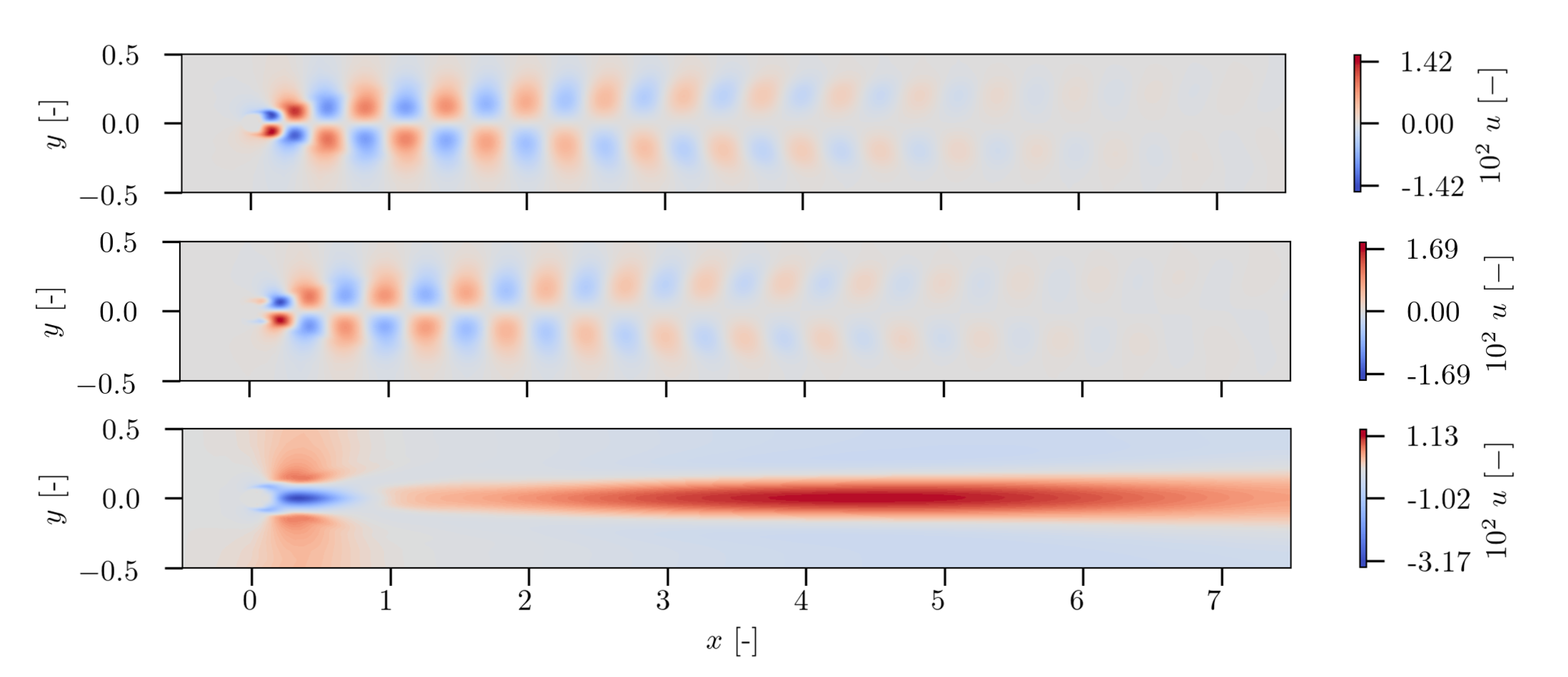
From the POD analysis, 2249 modes were obtained. Figure 19 shows the flow characteristics governed by three distinct POD modes: mode 1, mode 5 and mode 15. The lower POD modes capture the large scale flow structures. The higher the POD modes, the smaller the scale of the flow structures. The 1st POD mode captures the large flow dynamics at the beginning of the wake recovery at $x\approx 145\mathrm{m}$. This POD mode also indicates the development of vortex structures due to ground interactions of the flow at $x\approx 80\mathrm{m}$. POD mode 5 shows more detailed patterns. The flow dynamics of detached vortices near the ground at $x\approx 80\mathrm{m}$ is clearly shown. More downstream, a clearly visible mixing of the flow is present. The presence of the bade tip vortices as well as the wake of the wind turbine hub are slightly visible in POD mode 15. In the near ground region, the interaction of the blade tip vortices with the ground boundary layer and the sheared inflow, respectively, can be seen. It can be noticed that the vortex structures in the ground area increase more downstream. 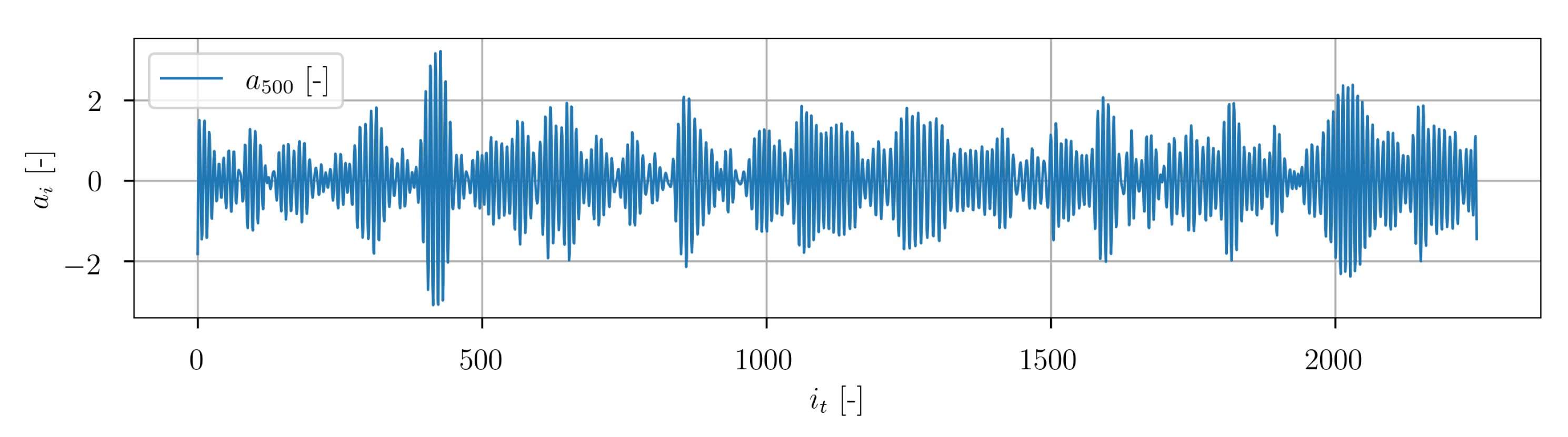The beginning of the wake recovery at $x\approx 145\mathrm{m}$ is also captured. Higher POD modes, corresponding to low eigenvalues, only capture some small scale dynamics. At POD mode 500, for instance, high resolution correlation structures in the turbine hub wake and in the upper region of the wake recovery are present.

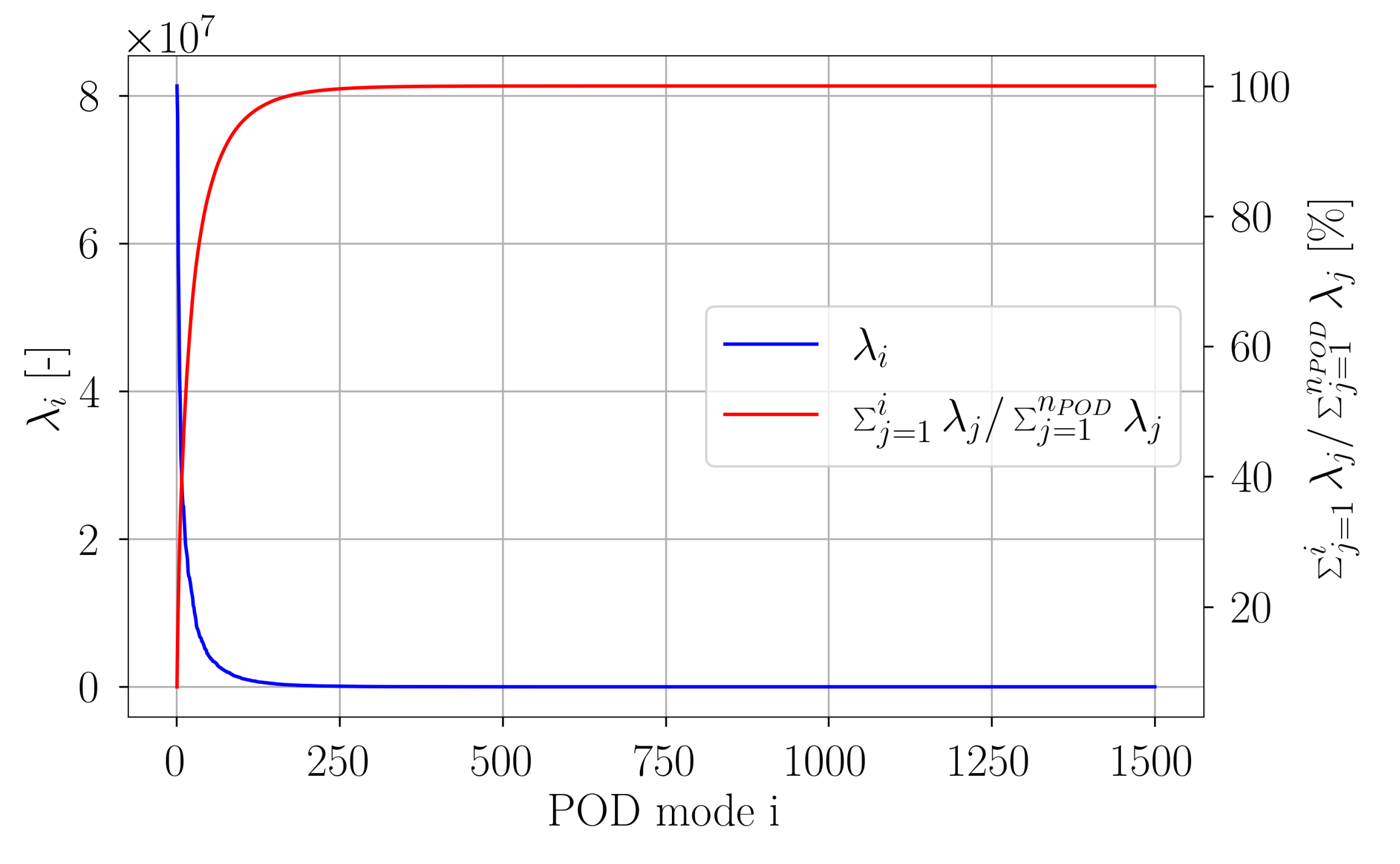
In Figure 20, the value of each eigenvalue is depicted. The accumulated fluctuation kinetic energy portion of the first i POD modes relative to the total fluctuating kinetic energy is shown. It can be clearly seen that the main portion of the fluctuation kinetic energy of the flow is captured by only approximately 10% of the POD modes. More detailed, around 90% of the fluctuation kinetic energy is captured by the first 22 POD modes, around 99% is captured by the first 198 POD modes. As observed in the case of the flow around a cylinder, the higher POD modes contribute no significant amount of fluctuation kinetic energy to the total amount.

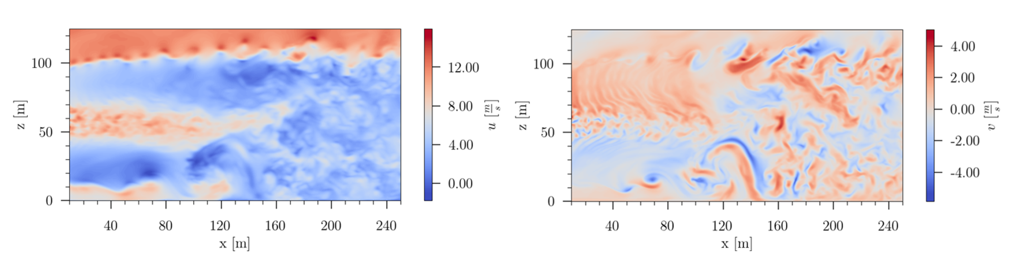
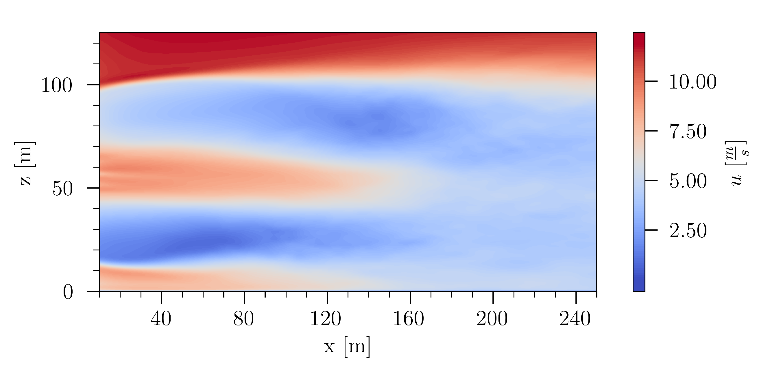
Considering the mean velocity field in Figure 21, some time averaged properties of the wake are revealed. The contour plot of u shows a clear delimitation between the unperturbed flow and the wake of the wind turbine. A distinct velocity deficit of the flow, which interacts with the rotor blades, is present. The wake of the turbine hub reduces more downstream and vanishes in the wake recovery region. In the lower region of the wake, the interaction of the blade tip vortices with the sheared velocity profile leads to instabilities more upstream than in the upper region of the wake, where the blade tip vortices evolve in a more delimited area. Approximately one rotor diameter downstream the wind turbine, the wake recovery is clearly visible. Highly turbulent structures lead to a significant mixing of the flow.

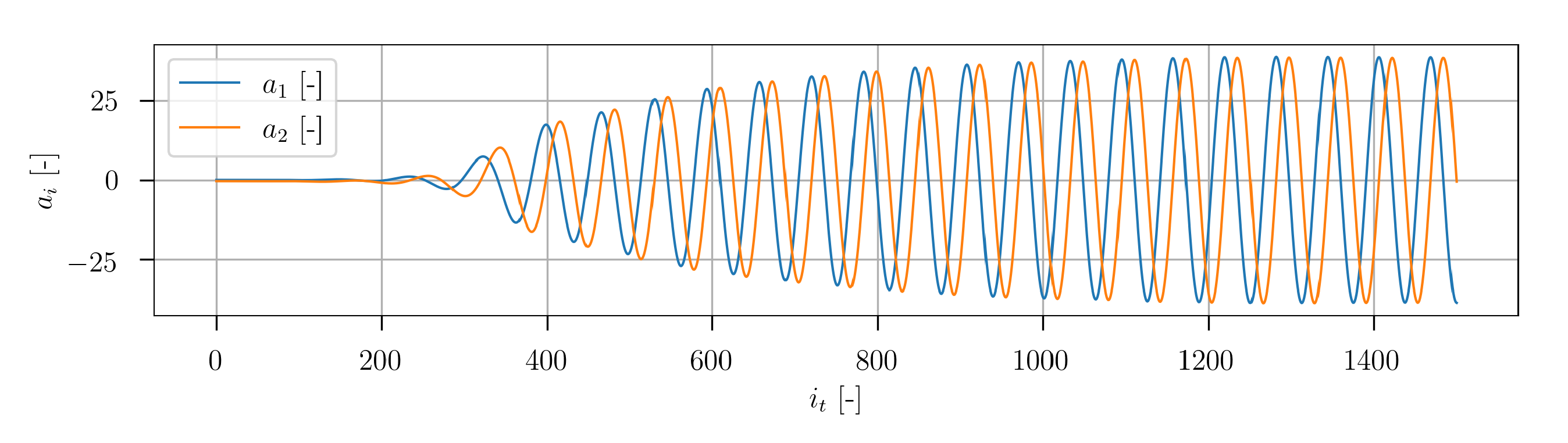
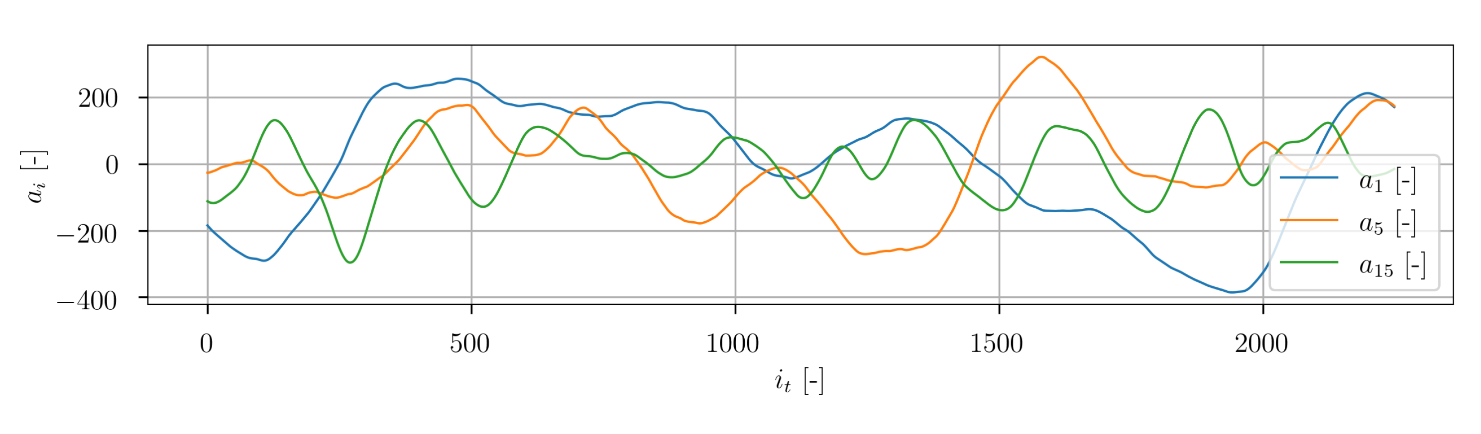
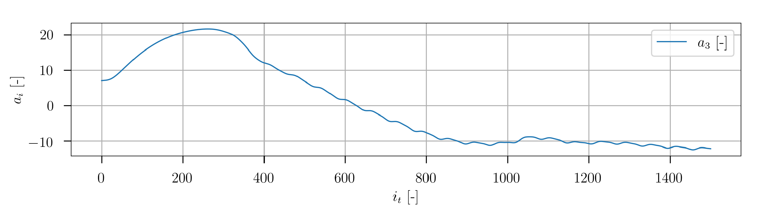
In Figure 22 the temporal developments of the POD coefficients of mode 1, 5 and 15 are depicted. A very transient character is clearly visible. The representative of higher POD modes is plotted in Figure 23. The signal exhibits significantly higher frequencies. In general, the temporal progression of the POD coefficients shows no obvious regular macroscopic patterns.

The results obtained from the POD reveal a significantly higher complexity of the dataset compared to the cylinder flow dataset. Different POD modes capture flow characteristics over a wide range of spatial resolution. This corresponds to the different turbulence length scales of the high resolution turbulent flow data. The temporal POD coefficients show no obvious regular patterns in their temporal progressions.

b.

Clustering and reduced order modeling

b.1

Based on k-means clustering

In this section, sparse sensor placement results based on the classification approach are presented. The adopted approach is similar to what has been done for the cylinder case in Section 3.1.1. Four different settings were tested according to Table 2.

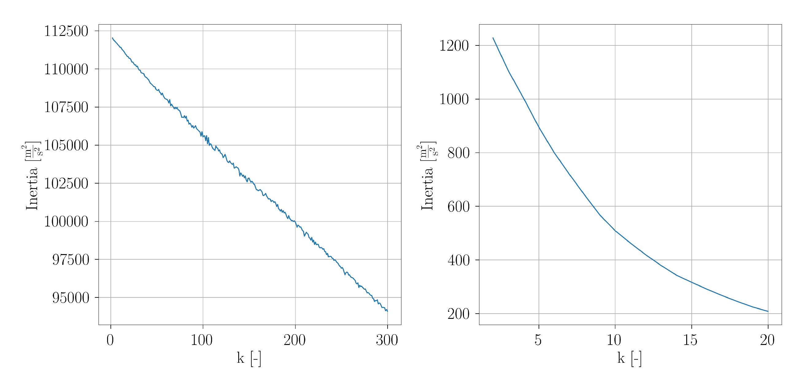
For setup 1, the inertia values obtained from k-means clustering are shown in Figure 24. It is clearly visible, that the curve exhibits no ‘elbow’. This can be caused by several reasons. The POD was conducted in the 2249-dimensional POD subspace and it is possible that the dimensionality is too high so that the distance metric of the k-means clustering becomes ineffective. This problem can be related to the curse of dimensionality (firstly introduced by Bellman [55]). It is also possible that an appropriate clustering can be achieved for a very high value of k, but it seems unlikely. A further possibility is the lack of enough snapshot data, i.e., not enough statistical information are available. Since, in this context a small k is desired, for setup 1, no reasonable results are obtained.

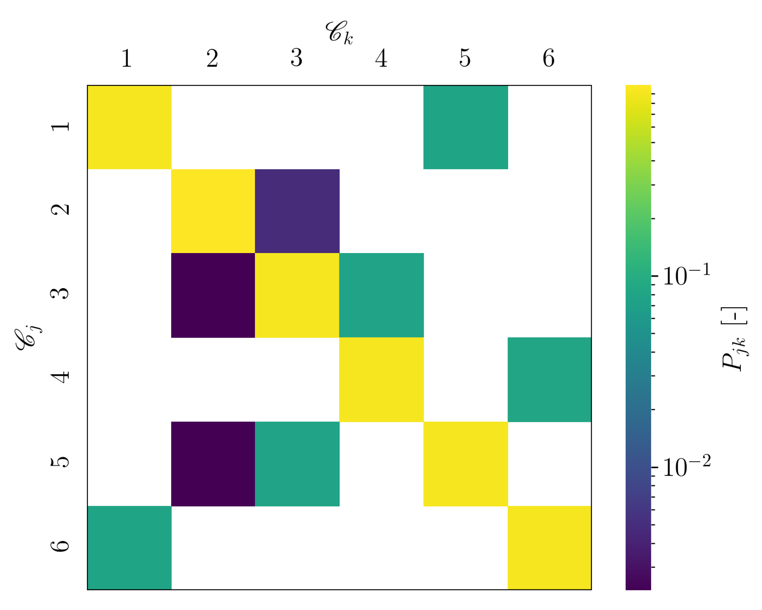
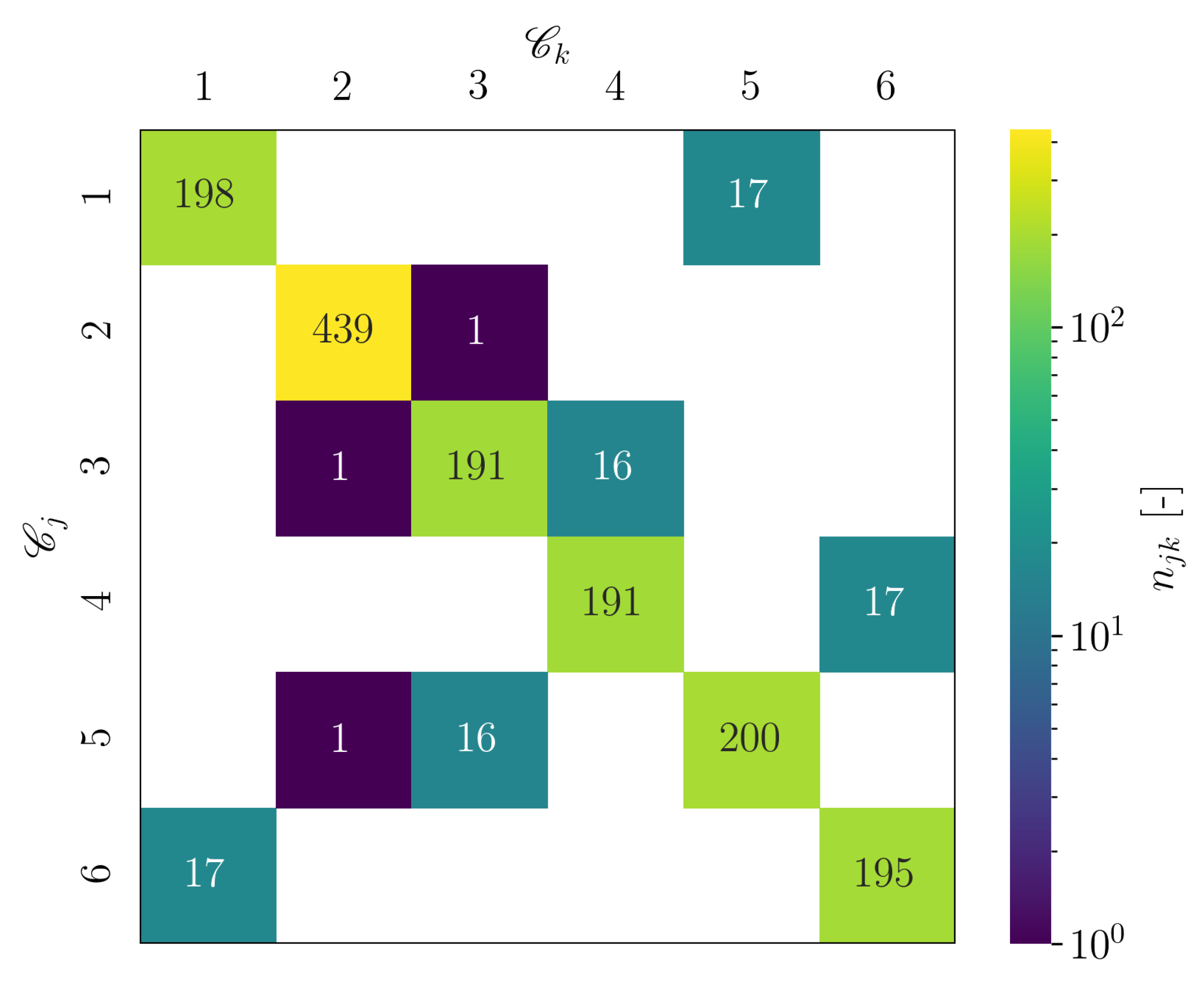
For setup 2, the plot of inertia over k is shown in Figure 24. With increasing k, it can be seen that the slope of the curve flattens. A slight elbow can be seen. In Figure 25, a visualization of the number of cluster transitions is given. The main diagonal entries show the number of transitions, for which the assigned cluster remains the same. The off-diagonal entries show the number of transitions, which occur between two different clusters. It can be seen that each transition between two different clusters only occurred once and twice, respectively. In contrast to the estimated dynamical system for the cylinder flow dataset, the estimated dynamical model of the wind turbine case corresponds rather to a chain. Hence, considering the complexity of the flow, the obtained reduced order model is likely not suitable for a subsequent application of SSPOC.

The inertia over k plots for setup 3 and setup 4 also indicate the presence of elbow (not presented in this paper). Similar to what has been observed for setup 2, all off-diagonal entries unequal zero showed solely the value one for the counted cluster transitions. Hence, again the dynamical models are rather similar to a transition chain. In this sense, the estimated reduced order models are also not suitable for a subsequent application of SSPOC.

A reasonable clustering of the snapshot data is necessary as a preliminary step before applying SSPOC since this technique requires labeled snapshot data. For setup 1 which considers all POD modes, the corresponding curve of the inertia over k shows no elbow. Based on the assumption that the k-means metric possibly will be more effective in case of a lower dimensionality of the POD subspace, only the first r POD modes were considered in setup 2–4 (and consequently only a part of the total fluctuating kinetic energy) in Table 2 to investigate the influence of the POD subspace dimensionality on the clustering results. Since no improvements were achieved for these setups, it can be depicted that considering even more POD modes (and consequently an even higher amount of fluctuating kinetic energy) will not lead to better results because this further increases the dimensionality of the corresponding POD subspace.

Furthermore, it was also attempted to reduce the dimensionality of the state space by means of spatial subsampling. For different values of subsampling factor, further evaluation was applied to the snapshot dataset. The POD was applied to the reduced dataset and subsequently k-means clustering was conducted for different values of k. The obtained plots of inertia over k indicate a constant descend of the curve for each subsampling factor. Hence, it was not possible to estimate a reasonable value of k.

b.2

Based on hierarchical agglomerative clustering

Since the standard k-means clustering is not suitable for the complex wind turbine case, the suitability of the hierarchical agglomerative clustering (HAC) was also tested. For each $k\in [2,100]\subseteq \mathbb{N}$, a HAC and subsequent estimation of the silhouette coefficients was evaluated. For this, the AgglomerativeClustering and silhouette_score implementation by scikit-learn [43] were chosen. The Euclidean distance was used for computing the linkage distance. A minimization of merged clusters variance was adopted as the linkage criterion.

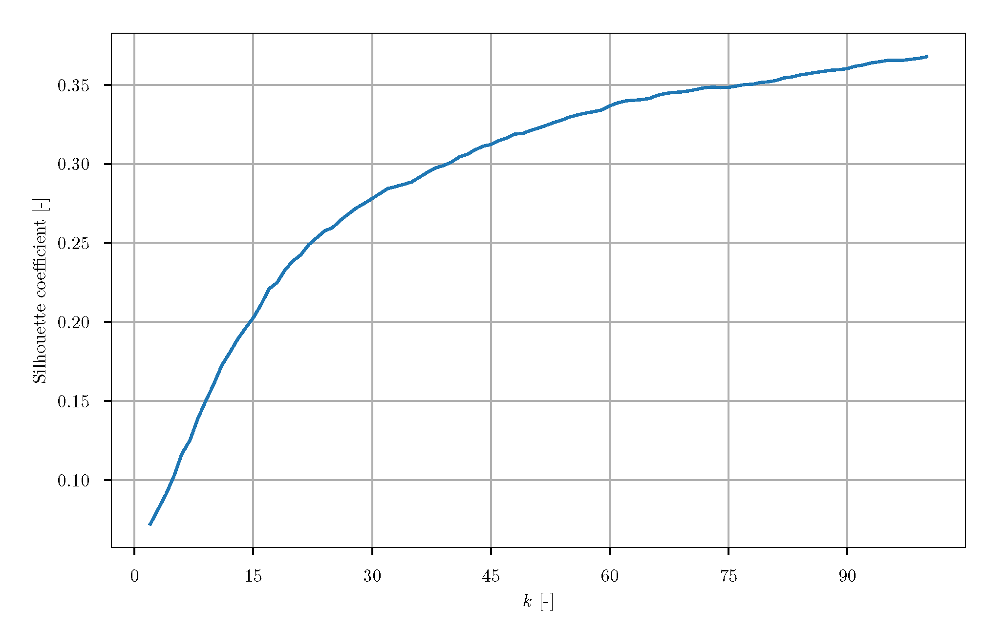
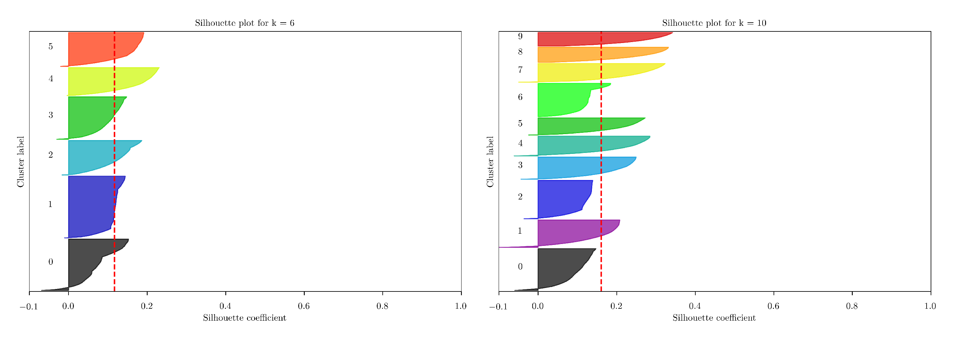
For increasing values of k, the silhouette coefficients (also known as overall average silhouette width) were estimated (Figure 26). It seems like the curve converges against an asymptotic value. Either a local maximum is located at a higher value of k or the maximum silhouette coefficient occurs at $k=m$, i.e., each snapshot is estimated as separate cluster comprising only one observation. In case of an optimal clustering, it is expected that the obtained curve exhibits a local maximum. However, this is not observed here. Instead, the silhouette plots of each k are visually evaluated. For example, in Figure 27 the silhouette plot for $k=6$ is shown. Each silhouette shows a narrow contour. This shows that in each cluster only a part of the points is clustered appropriately. It can be further seen that the silhouette coefficients do not exceed a value of around $0.2$. Ideally, the values are close to one. The red line denotes the overall averaged silhouette width. The given contour plot shows that no reasonable clustering of the snapshots can be estimated. Similar observations can be made for $k=10$ as depicted in Figure 27. The silhouette plots for the remaining values of k are of similar patterns. Hence, no reasonable results were obtained. Therefore, this method is not suggested for further evaluating the complex wind turbine case.

b.3

Based on Gaussian mixture model

The main weaknesses of k-means are the necessity of circular clusters and the lack of probabilistic cluster assignment [56]. To overcome these issues, the Gaussian mixture model (GMM) was considered. Different settings were considered as listed in

Table 8. Different settings for Gaussian mixture model.

Setup	Data	r	${\mathit{k}}_{\mathit{max}}$
1	raw	$n_{POD}$	10
2	normalized	$n_{POD}$	10
3	raw	71	40
4	normalized	71	40
5	raw	198	25
6	normalized	198	25

. Three different numbers of considered POD modes were used: $r=2249$ POD modes (no truncation), $r=71$ POD modes and $r=198$ POD modes, which correspond to $100\%$, ≈90.0% and ≈99.0% captured fluctuation kinetic energy, respectively. For each r, both cases of raw and normalized snapshot data were taken into account.

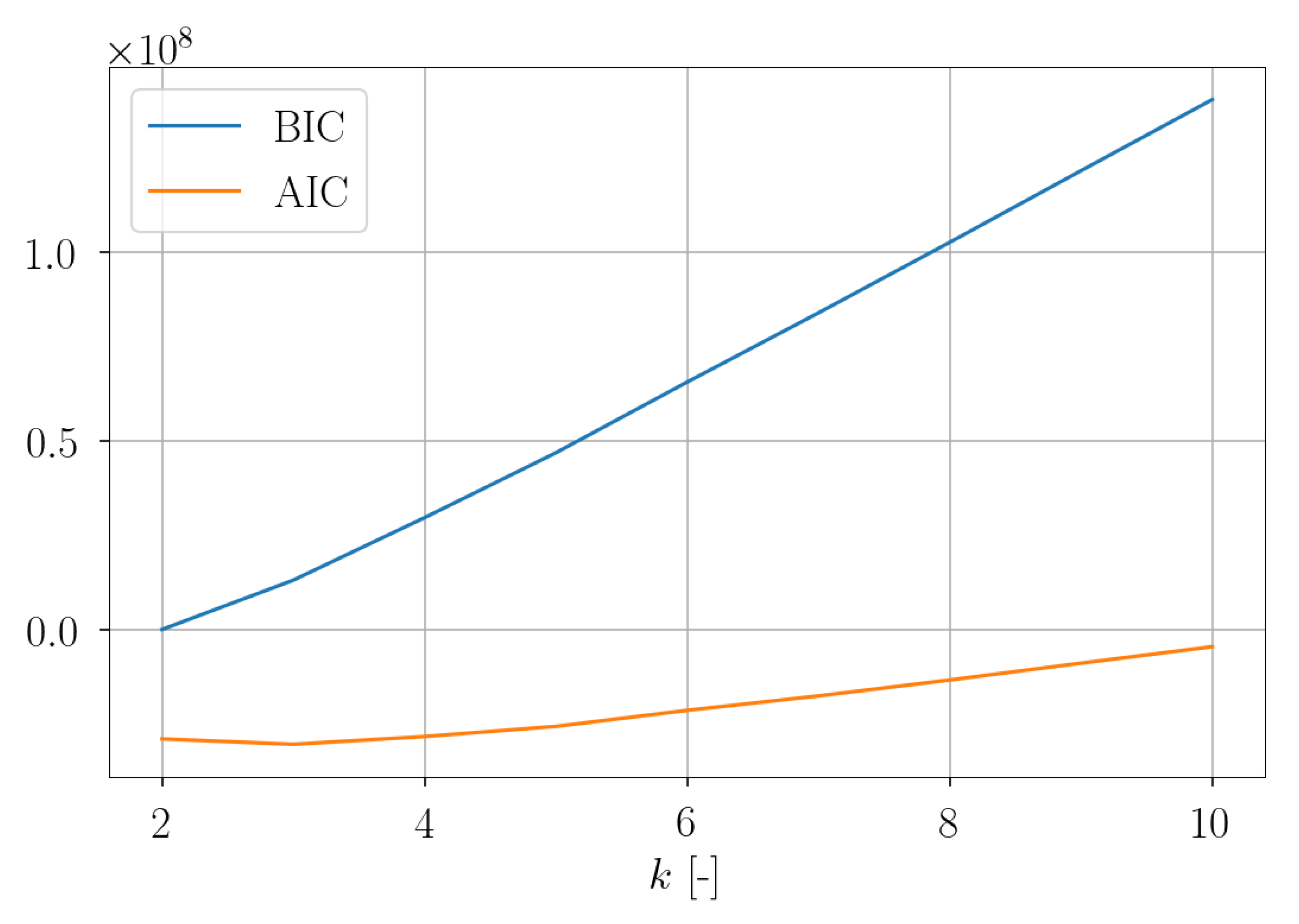
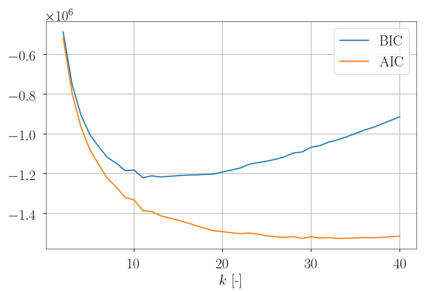
For the 1st setup, the obtained values for the Akaike information criterion (AIC) and the Bayesian information criterion (BIC) are shown in Figure 28. It can be seen that both raise for increasing values of the number of clusters k. To be exact, in the context of GMMs k denotes the number of used Gaussian probability distributions in the POD subspace, not the number of clusters. It is desired to minimize the AIC and BIC. For the AIC, a local minimum was estimated for $k=3$. Here again, the number of transitions from cluster ${\mathcal{C}}_k$ to cluster ${\mathcal{C}}_j$ were estimated. The corresponding heatmap (not shown here) indicates the off-diagonal entries only values of zero, one and two. Hence, as argued for the k-means clustering, no suitable dynamic model was also obtained here. The inertia over k has a monotone decreasing progression. Consequently, it is not suitable for applying the elbow method.

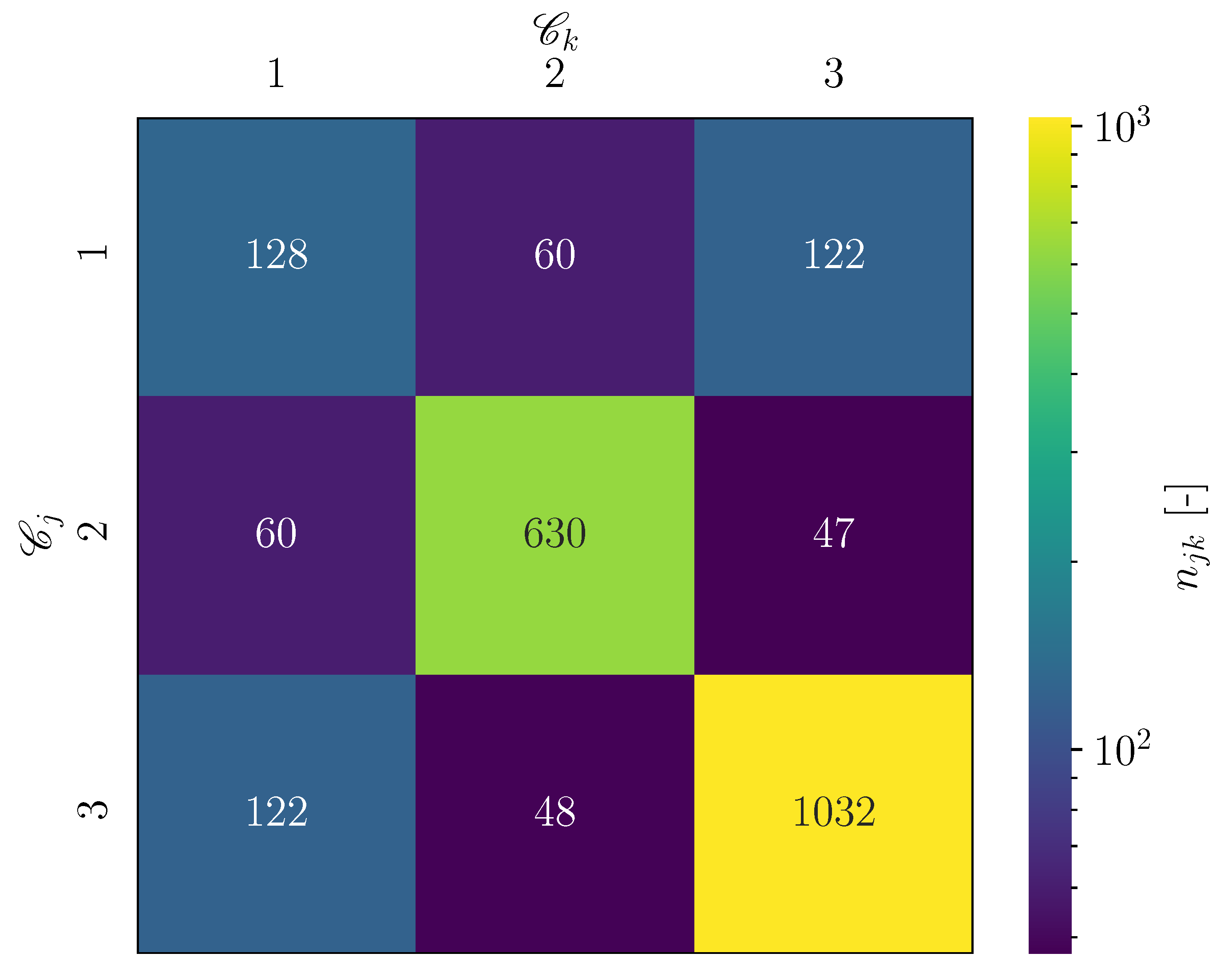
For the 2nd setup, the plot of the AIC and BIC over k show a similar progression. Also here, for the AIC a local minimum was estimated for $k=3$. Interestingly, the estimated CTM was not sparse. In Figure 29, an equivalent visualization of the number of transitions from cluster ${\mathcal{C}}_k$ to cluster ${\mathcal{C}}_j$ is given. 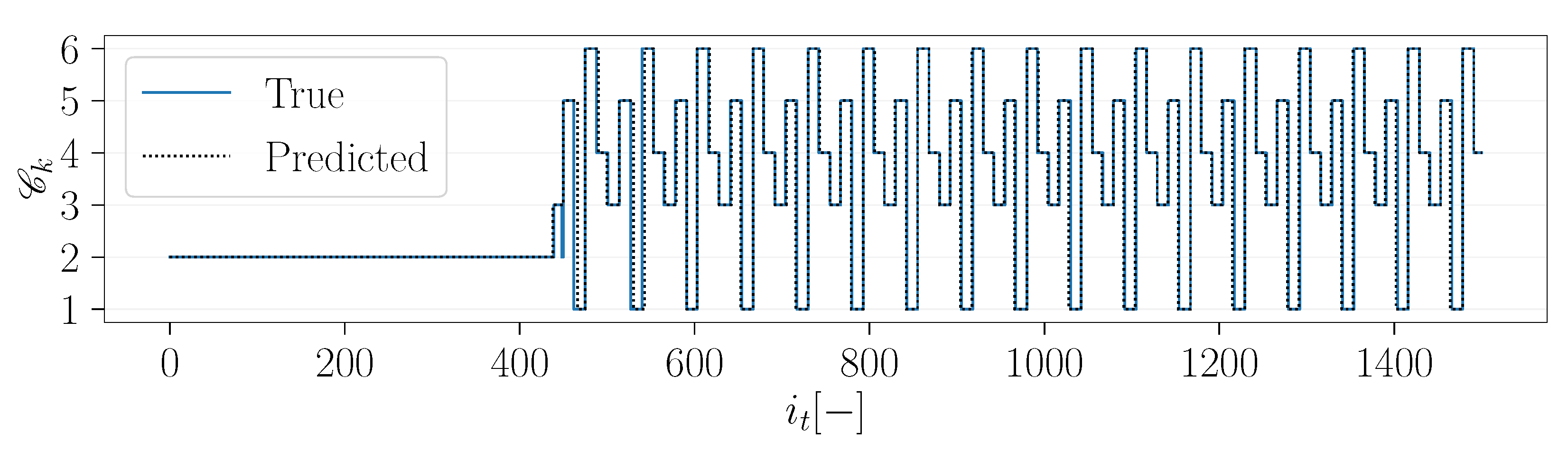For a further evaluation of the obtained results, the progression of the assigned cluster over $i_t$ was considered. As can be seen in Figure 30, the temporal progression shows a rather random character, indicating that the clustering leads to no reasonable partition of the POD subspace. Furthermore, it seems unlikely that the highly complex flow around a wind turbine can be properly represented by means of a reduced order model containing only three states.

Since no reasonable results were obtained also for the remaining setups (3–6), in the following only the relevant information is summarized. For the 3rd setup, a local minimum of the BIC at $k=30$ was estimated. The obtained CTM shows the same structure as for setup 1. As depicted in Figure 31, a local minimum of the BIC was estimated at $k=11$. Again, the CROM approach led to no useful results. In the case of setup 5 and 6, a local minimum of the BIC was estimated at $k=13$ and $k=6$, respectively. However, no meaningful reduced order model of the snapshot data was obtained.

In summary, for the wind turbine data set, the pursued approaches of CROM in combination with SSPOC provide to no reasonable results. It can be seen that the high complexity of the wind turbine data set makes it is very difficult to estimate a low-order model representation of the flow field without significant loss of information. These findings coincide with the studies of D’Agostino et al. [24] for a four-bladed propeller wake. They applied k-means clustering to the phase-locked vorticity snapshots of a four-bladed propeller wake. Considering the entire wake (near- and far-wake), reasonable clustering results were achieved. Taking only the very near wake into account, no reasonable clustering results were obtained, which means that a single cluster was estimated as optimum snapshot partitioning. The results of the present work are inline with the results obtained in [24]. This indicates that clustering of snapshot flow data is in general only reasonable for macroscopic flow structures.

c.

Sensor placement based on reconstruction

c.1

Variation of number of basis modes

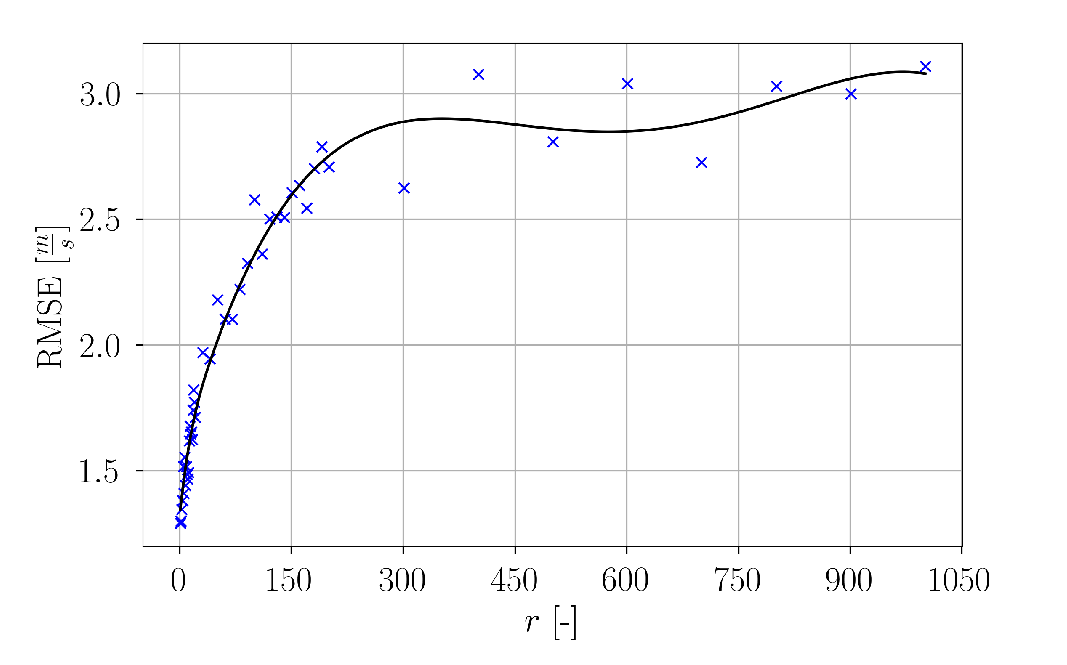
The estimated reconstruction errors of all setups are summarized in Figure 32. The computed reconstruction error values for each r are depicted as blue crosses. The data points were interpolated by means of a spline of fourth order. In the range of $r=1\dots 150$, a steep increase of the reconstruction error can be observed. However, for higher values of r the curve flattens. One might assume that the reconstruction error for low values of r will be higher, since fewer flow characteristics will be captured and consequently the reconstruction will be less accurate. Consequently, the reconstruction error will decrease for higher r. However, here the opposite is observed. By increasing the number of basis modes for snapshot representation, the reconstruction error rises and seems to approach an asymptotic value for very high r. This is caused by the fact that for low r, the small scale flow structures are not captured for reconstruction. Consequently, the true values fluctuate around a rather steady progression of the predicted values. In the case of higher r, also small scale flow structures are reconstructed. Hence, both the true and the predicted signal exhibit a higher degree of fluctuation, which partially increases the difference between true signals and predictions. As mentioned in the POD analysis, around 99% of the fluctuation kinetic energy is captured by the first $r=198$ POD modes. This value coincides with the range of r in which the curve flattens. Therefore, for 198 employed sensors, reconstructions of the snapshot data can be made without a significant loss of information.

c.2

Estimation of the smallest possible set of sensors

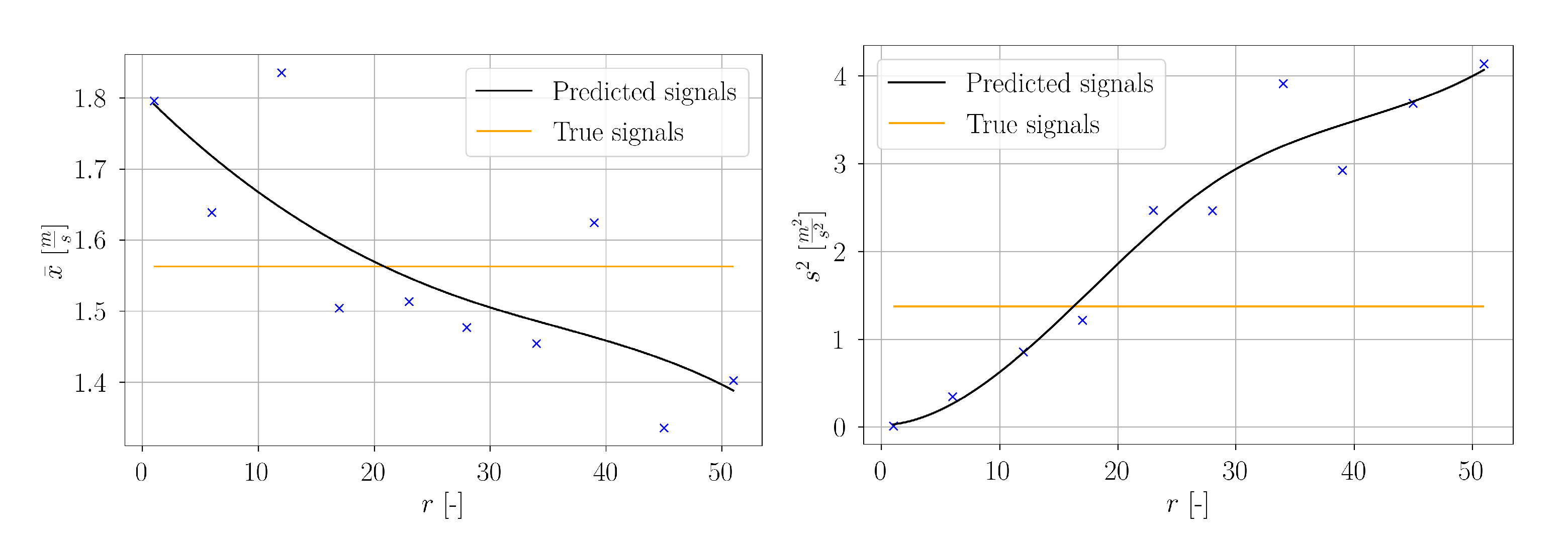
In the context of this work, a minimum number of sensors is desired. Consequently, $n_s=198$ is considered as too high. For estimation of an appropriate value of $n_s$, in the following, another approach was pursued. At discrete spatial locations, predicted and true signals were evaluated for different values of r to achieve a maximum possible agreement of the statistical properties with the true signals.

At first, the signal mean averaged over all measurement points and all velocity components according to Equations (11) and (17) for true and predicted signals, respectively, were considered. In Figure 33, the estimated values are denoted as blue crosses. An interpolation curve was estimated by means of a cubic spline. For low values of r, the total mean of the predictions is higher than for the true signals. At around $r\approx 20$ they are equal and for higher r the prediction mean is lower than the true one. Furthermore, the signal variance averaged over all measurement points and all velocity components according to Equations (14) and (20) for true and predicted signals, respectively, were also considered. It is clearly visible that an increase of r goes hand in hand with a higher variance of the predictions. At $r\approx 16$ the overall variance of the predictions equals the true test data variance. From this basis, a number of 20 sensors was selected as an appropriate value. The estimated sensor locations were used for further studies.

c.3

Final sensor placement

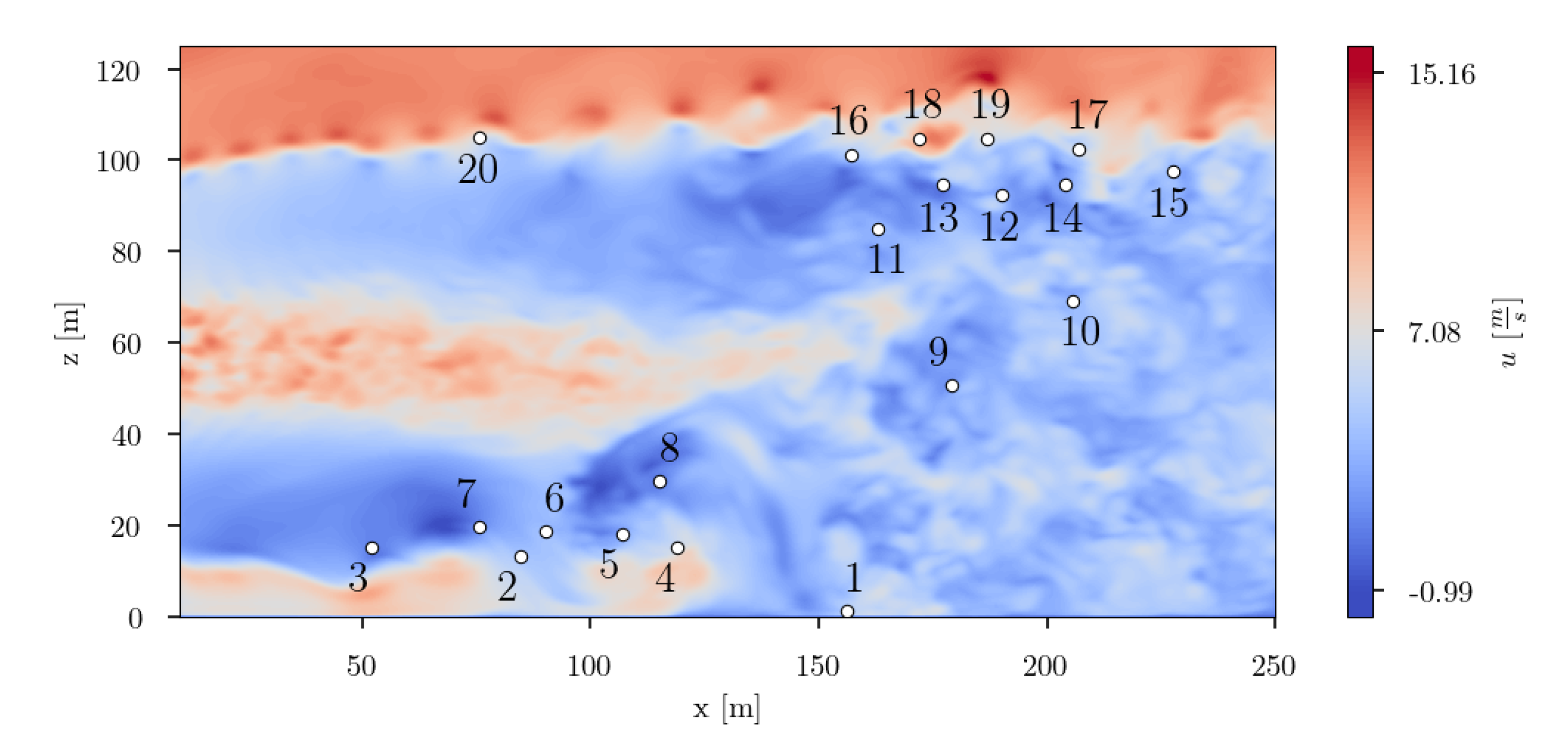
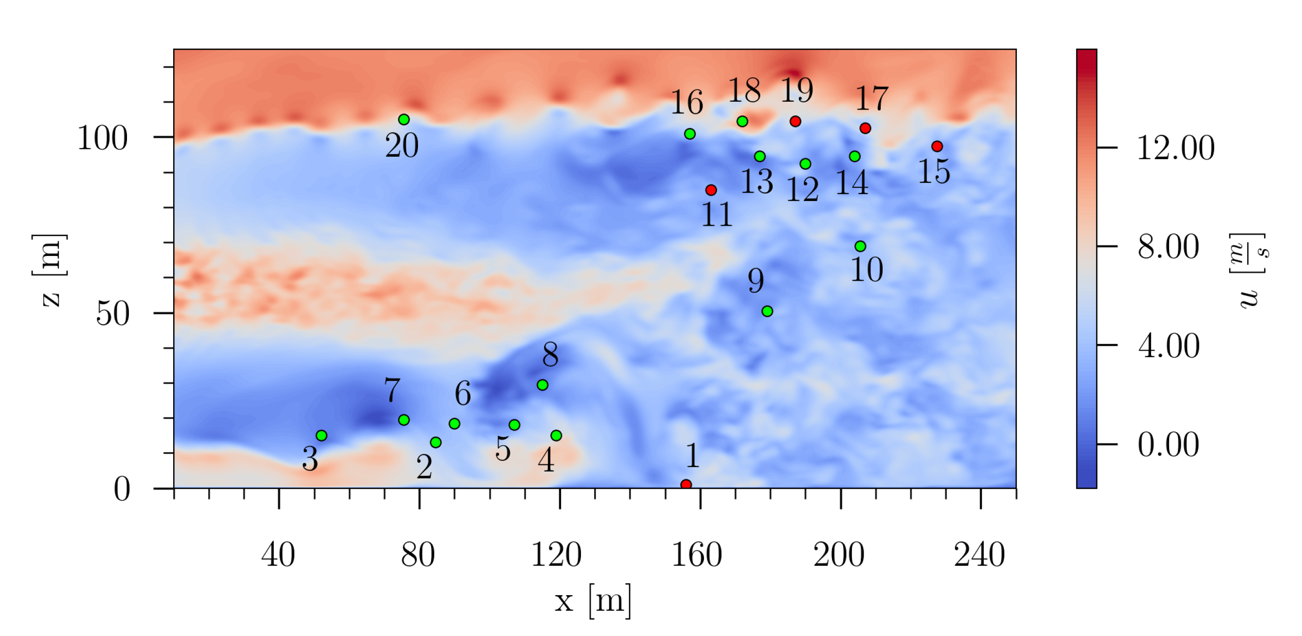
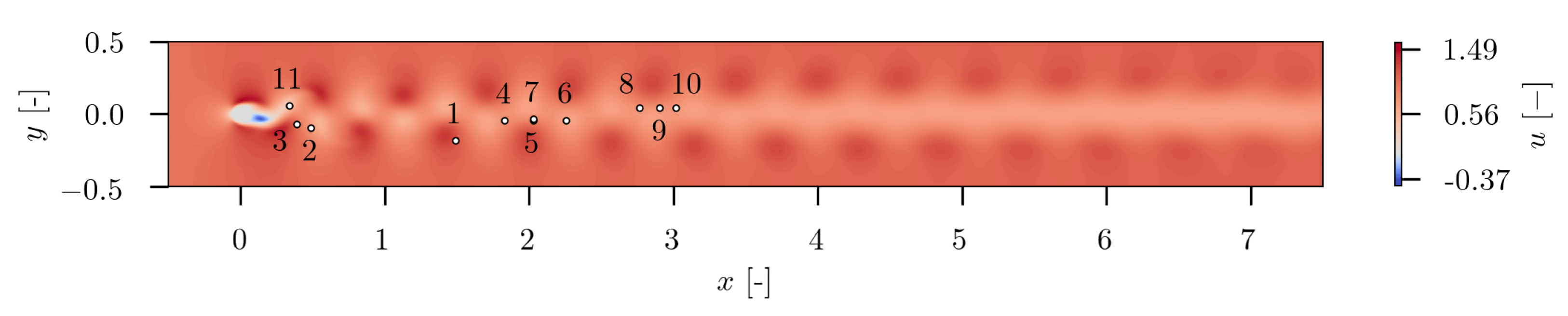
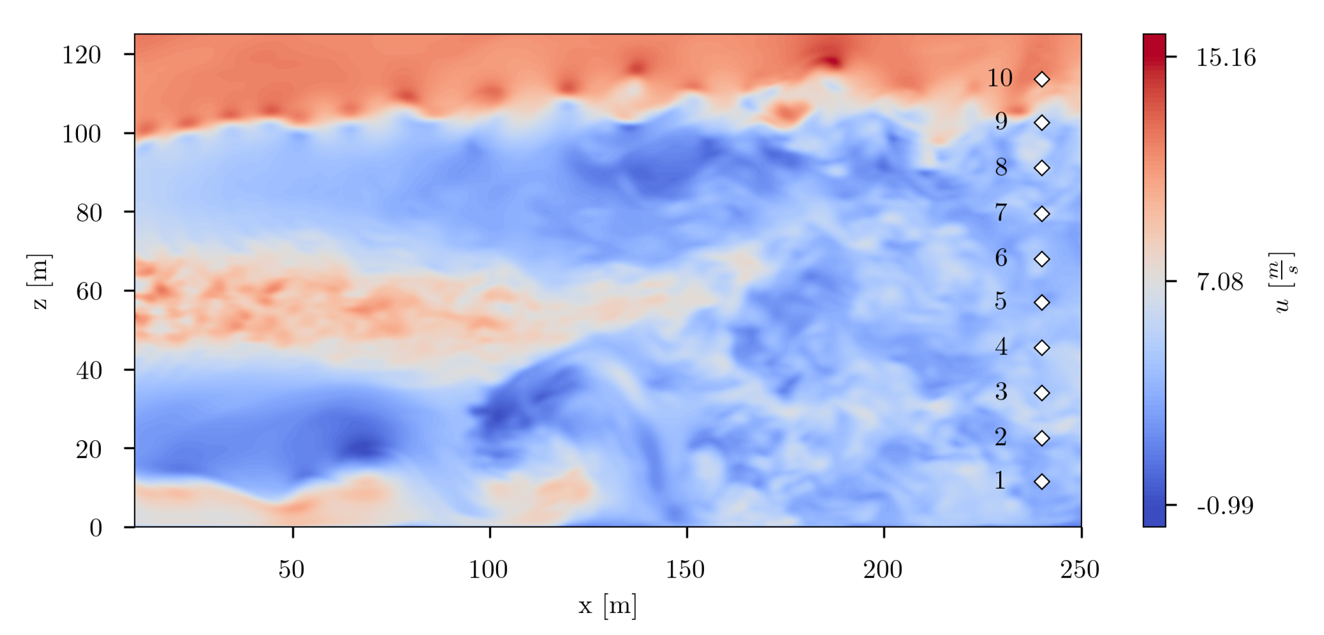
In Figure 34, the twenty finally estimated sensors are depicted. Taking a look at the spatial distribution of the sensors, it can be clearly seen that the sensors are not equally distributed. They are agglomerated in two distinct regions, and a single sensor is placed in a third region. The sensors in the lower part of the flow field domain are located in the area, where distinct large scale vortex structures evolve. By means of SSPOR the transition area in the near ground region was estimated as one of the most informative location for sensors. The second cluster of sensors is located in the region in the upper right of the flow domain. In this region, the transition area of the wind turbine wake can be identified, where wake recovery begins. This region seems also to be most informative. Additionally, in the upper left of the flow domain one single sensor is placed. This one could possibly indicate the region where the pairing of tip vortices occurs.

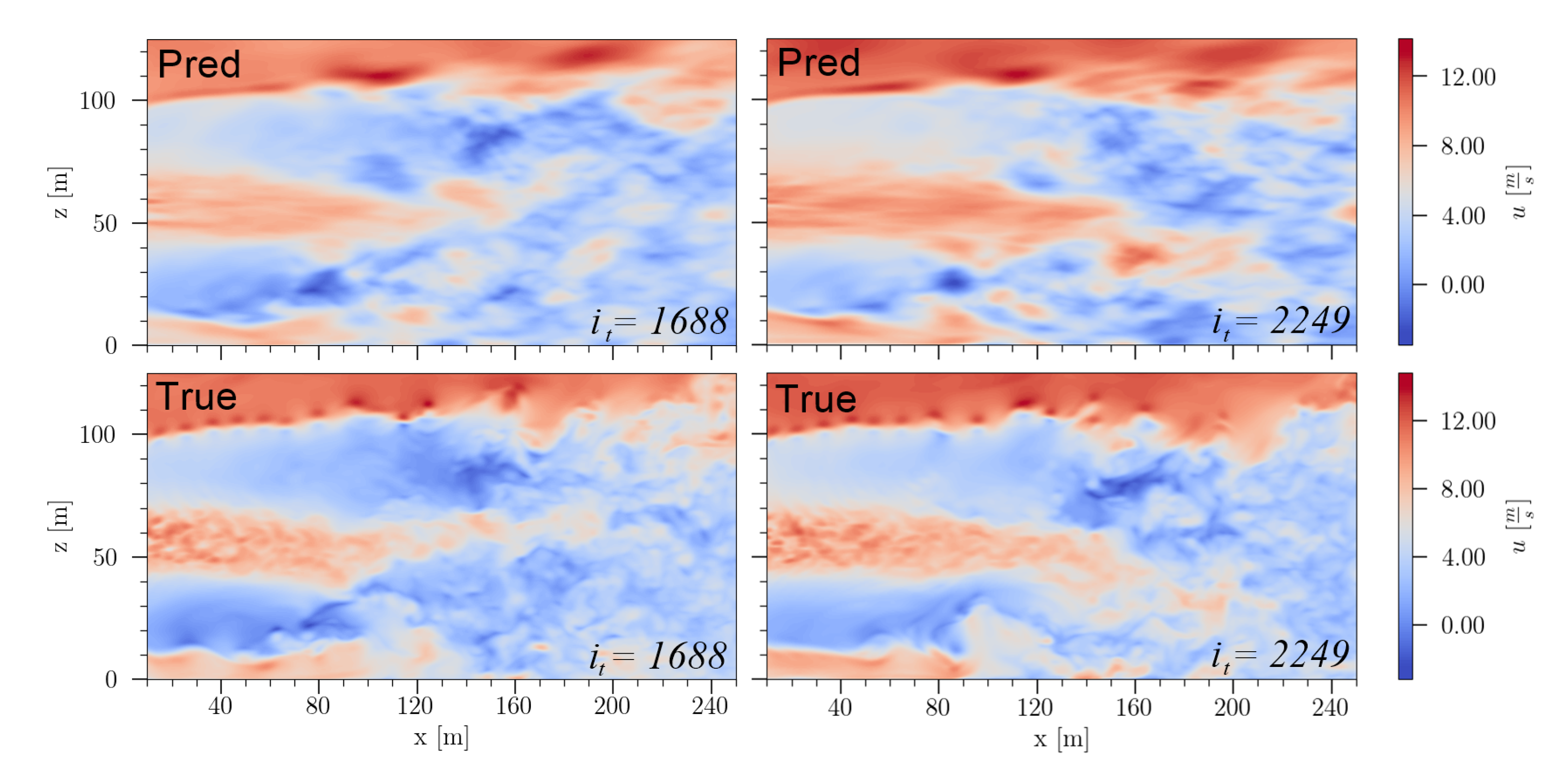
In Figure 35, the reconstructed velocity field based on the sensor measurements for two different time instances is presented. It is apparent, that the predicted velocity fields contain less small scale turbulent structures. However, the main characteristics of the flow field are preserved: the wake area of the wind turbine hub, the large vortex structures in the ground area at $x\approx 70\dots 130\mathrm{m}$, the distinct velocity deficit of the near-wake, the clear distinction to the unperturbed flow and the beginning of the wake recovery. The fact that the predicted flow field snapshots show less small scale turbulent structures is because the POD modes used as basis modes for SSPOR do not capture these very small scale flow structures. Note that increasing the number of the employed modes increase the computational effort and the number of data and sensors, and is counter productive for real applications.

3.2.2. Wake Prediction

a.

Standard setup

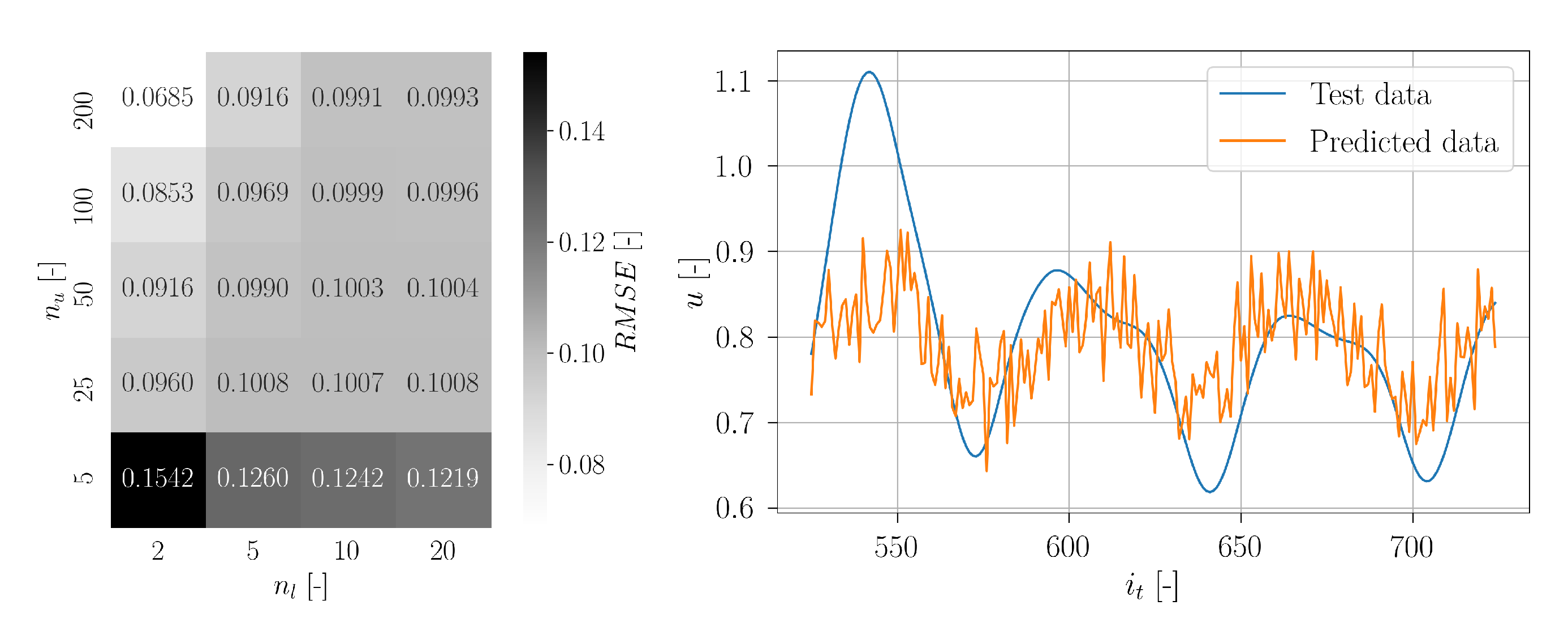
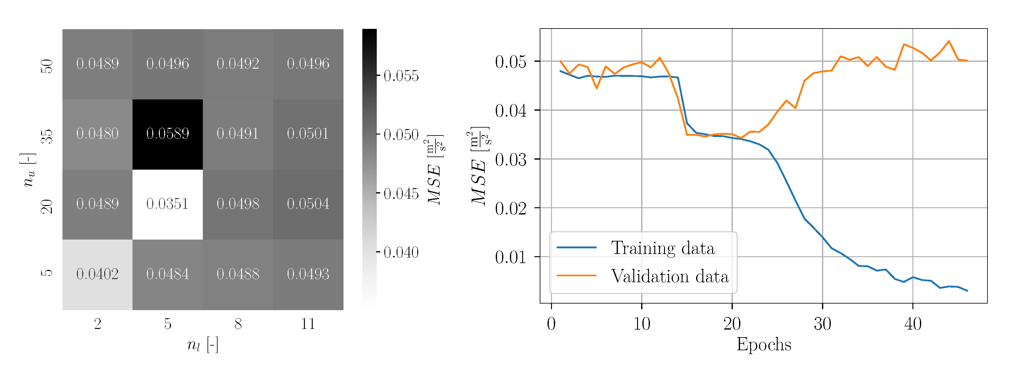
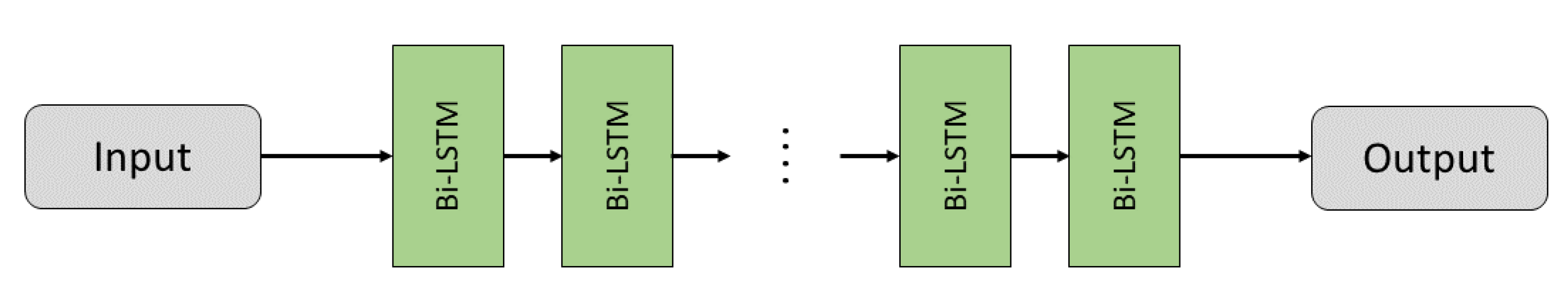
The obtained validation loss values for each parameter grid point are visualized in Figure 36. It should be noted that the MSE was computed for the normalized data, which explains the perceived really low values. The best result was estimated for $n_l=5$ Bi-LSTM layers and $n_u=20$ units per layer. Interestingly, for $n_l=5$ and $n_u=35$ the maximum MSE was obtained. The remaining values of the parameter grid reveal no regular pattern and slightly vary around a moderate value.

With the estimated optimum hyperparameters, a subsequent training was conducted. The corresponding learning curve is depicted also in Figure 36. It can be seen that no significant learning progress is achieved for the first twelve epochs. However, around epoch 15, the training and the validation loss drops significantly. For epoch 21, the global minimum of the validation loss was estimated and the corresponding Bi-LSTM network was saved as final model. For further epochs, the training loss decreases further and the validation loss increases, which shows an indication of overfitting. The relatively constant development of the loss values for the first epochs demonstrates that the training algorithm has some difficulties to find a reasonable direction for the gradient descent. This is caused by the unsuitable window size of the time series for the standard setup, challenging the Bi-LSTM to learn the data. For training of the Bi-LSTM networks, the Adam algorithm was applied enabling adaptive learning rates. This explains the smaller number of epochs compared to regular Stochastic Gradient Descent. Using the network weights corresponding to epoch 21 with the minimum validation loss—not the weights for the last epoch—ensures an optimal trained network without overfitting. The limited number of available snapshot data results in a limited learning success of the Bi-LSTM networks. This explains the remaining difference between training and validation loss for epoch 21, as well as the limited prediction accuracy. The CFD datasets were obtained from computationally expensive DDES simulations, even less than 10 min physical time for the complete statistics. The wind turbine is exposed to complex turbulent flow in combination with shear and yaw [10]. Furthermore, the rotor operates at a relatively large induction factor [10]. Thus, the prediction becomes very challenging. However, this is actually what the reality is in wind turbine operation, especially for fast-controller actions due to incoming wind, e.g., pitch response control. To account for this drawback, a modification in the method was made by adopting an adjusted window size based on the autocorrelation approach. This way, the prediction accuracy can be improved significantly but still maintaining a reasonable computational cost.

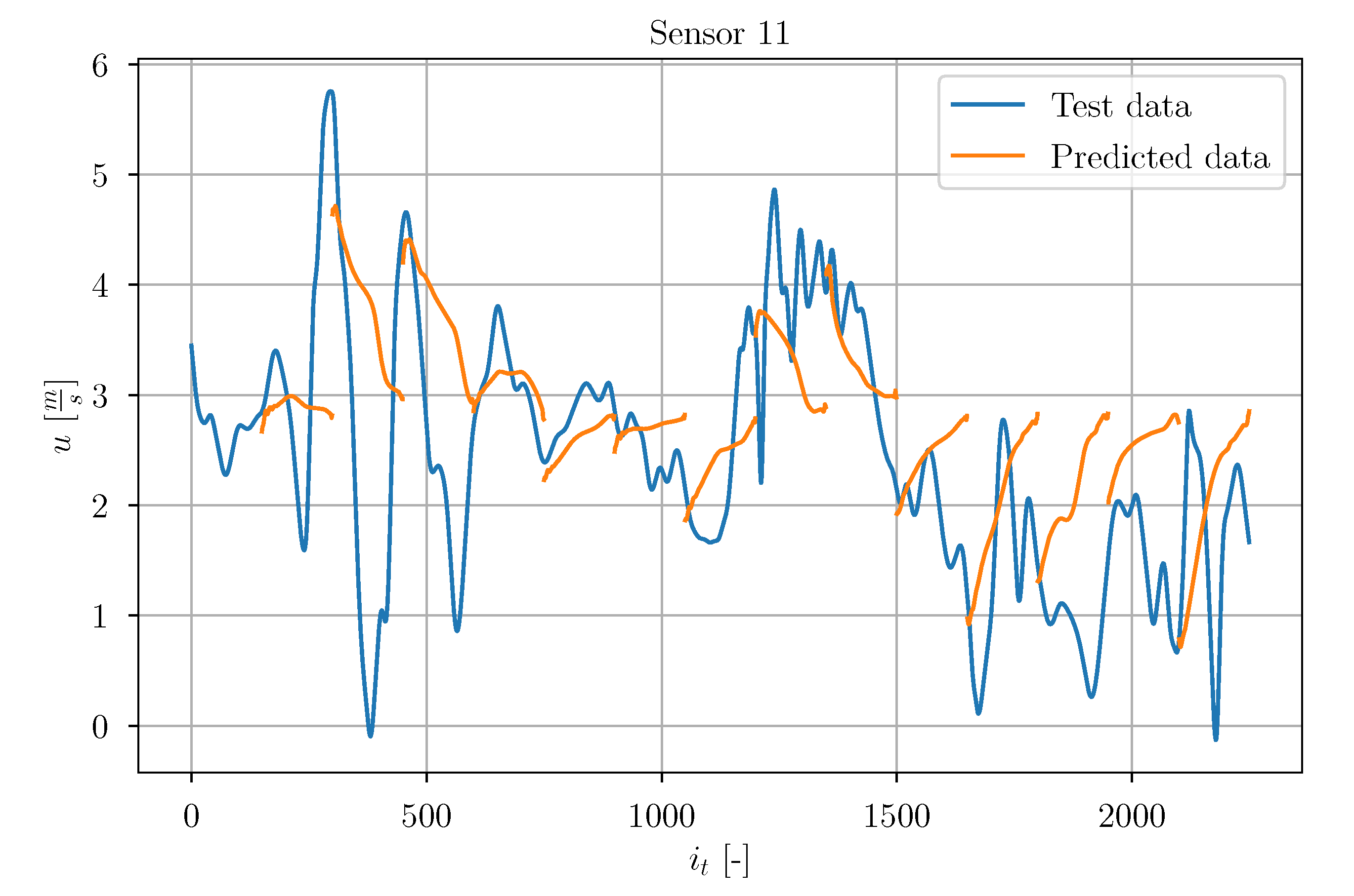
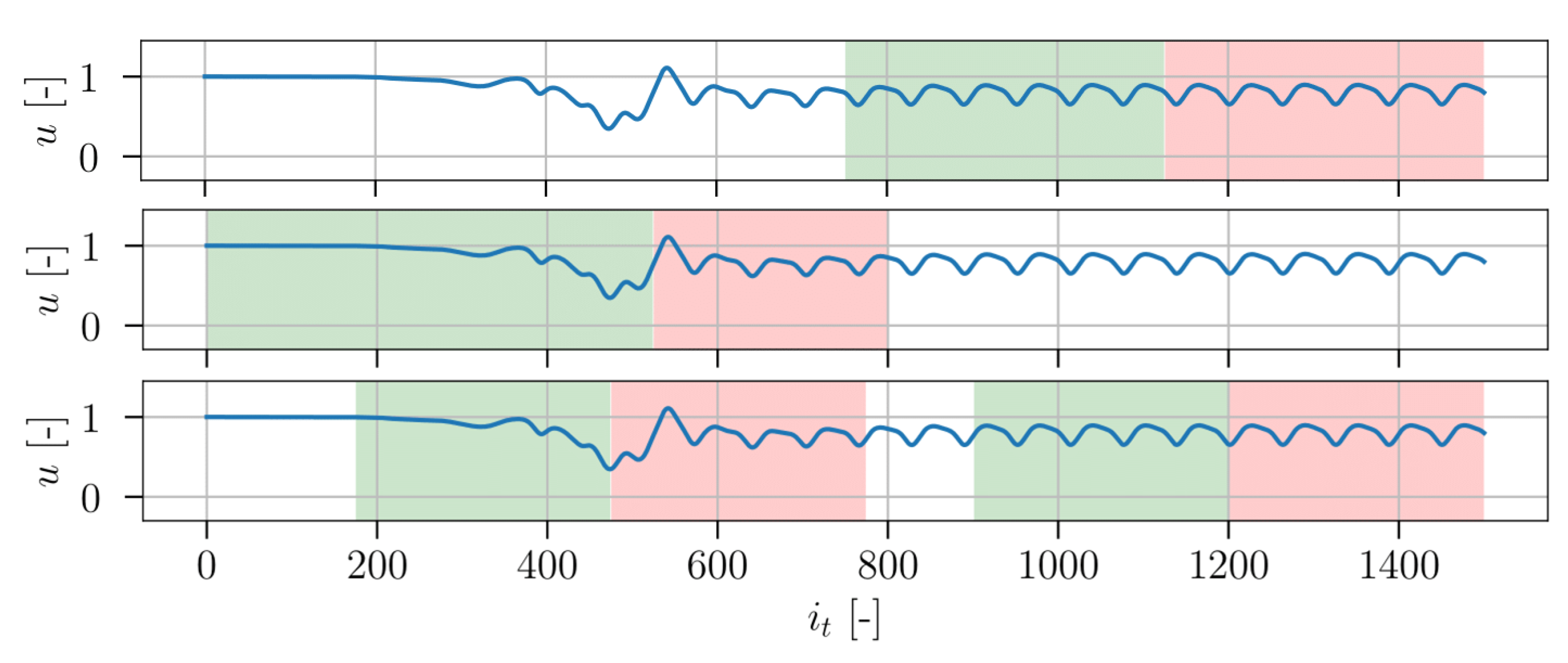
With the final model, predictions of the test data timeseries ${\mathit{y}}_{test}$ were made. As an example of the prediction, in the following the obtained results are discussed for sensor 11 (randomly chosen among other sensors). In Figure 37, the true test data signal is depicted together with a set of chronologically consecutive predicted timeseries. On a first sight, the predictions show no significant accuracy. It is noticeable that most of the predicted timeseries seem to strive towards $u\approx 3$ m/s. Some of the predictions seem to forecast some trend of the true signal, but there are also predictions which do not coincide with the true timeseries.

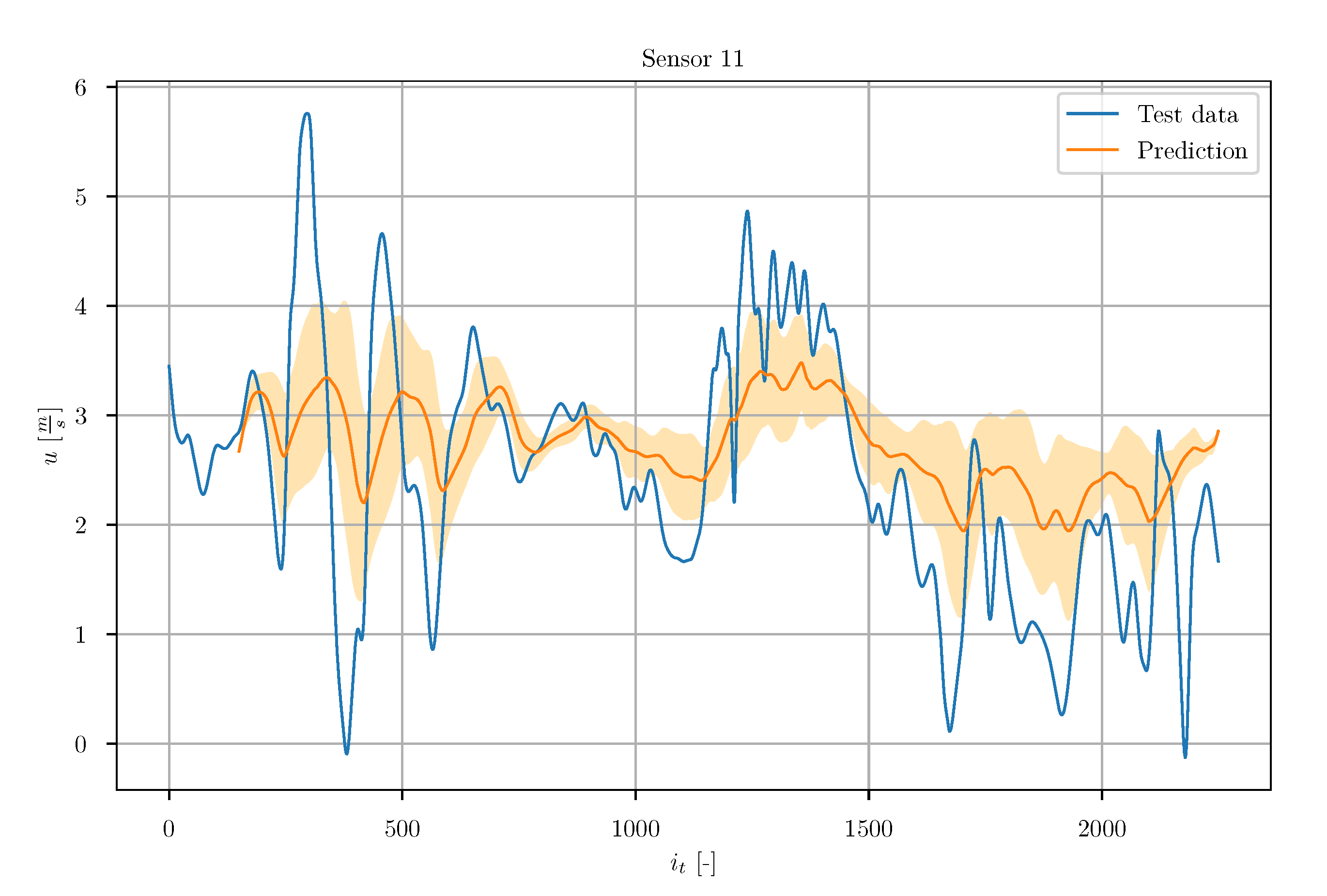
Furthermore, for a general impression of the prediction accuracy and consistency, all predicted test data timeseries were averaged. This means, for each instant, the mean of all available predicted observations from different timeseries was calculated. Additionally, the corresponding standard deviation was computed. In Figure 38, the averaged timeseries (orange) are shown together with the true signal of sensor 11. The transparent orange band indicates the standard deviation. The predictions show a large uncertainty. It can be seen that the predictions capture some tendencies of the true signal, but the overall averaged prediction is not performing well against the true signal. Furthermore, the uncertainty is relatively high.

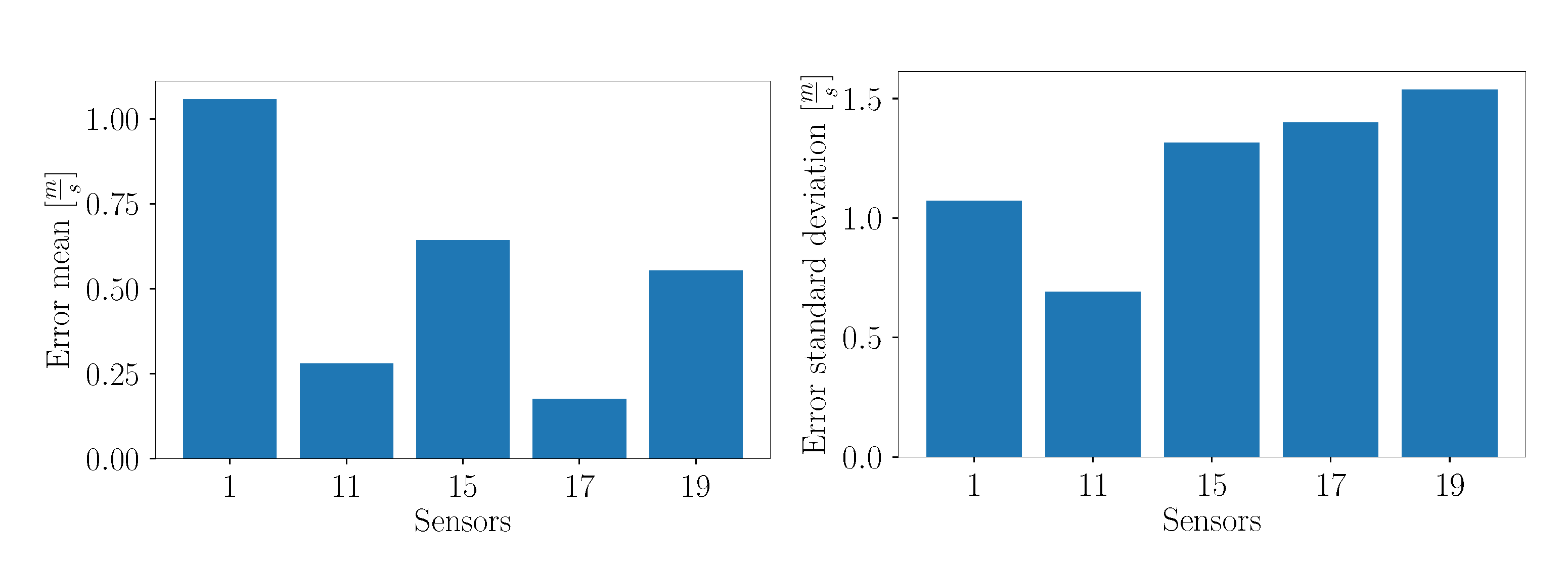
Considering the overall error mean of each test sensor in Figure 39, it can be seen that sensor 1 exhibits the largest error. This can be explained by its location in the flow field. In contrast to the other test sensors, sensor 1 is located relatively far away from other training sensors, whereas sensors 11, 15, 17 and 19 are located in the cluster of sensors in the upper right part of the flow domain. It can be concluded that the measurements of closely placed sensors are more similar due to coherent structures of the flow, and hence it is easier to make predictions at locations which lie nearby training sensors. Interestingly, the values of the error standard deviation of sensors 15, 17 and 19 are higher than for sensor 1, although sensor 1 is more distant to the training sensors. This could be explained by the fact that sensor 1 is located nearly to the ground, where no large fluctuations are expected. The other sensors are placed in the wake recovery region, where highly turbulent structures are present. Sensor 11 exhibits the smallest error standard deviation, as depicted in Figure 39.

b.

Adjusted window size

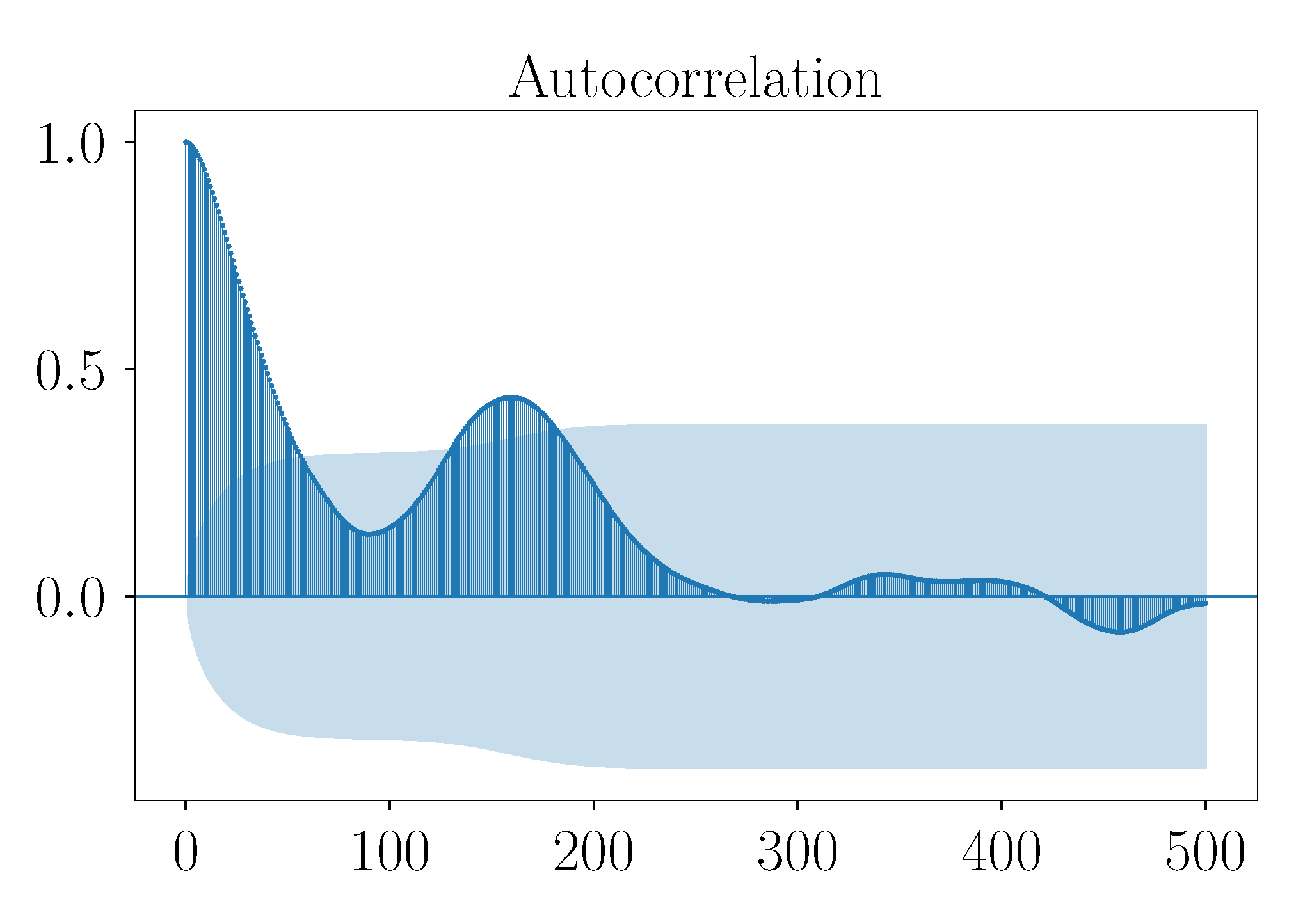
As a brief example, in Figure 40, the autocorrelation function (ACF) of the measured velocity component in x-direction at sensor 11 is depicted. The dark blue contour represents the autocorrelation values over the number of lags, and the light blue area represents the confidence interval. Correlation values inside the light blue area are regarded as not statistically significant. It can be seen that for low lag values the correlation values are high and decrease slowly for higher lag values. Furthermore, fluctuations are present. This progression of the ACF indicates a non-stationary timeseries showing a certain seasonality and also a trend. The frequency of the seasonal pattern can be approximated by the distance between two local maxima [57]. However, for higher lag values the seasonality pattern vanishes. It can be seen that the ACF exhibits no strict periodic patterns. This is in accordance with the fact that the underlying set of snapshots show a highly turbulent flow characteristic. Furthermore, despite the presence of some seasonality patterns, for high lag values the correlation values lie within the blue area, i.e., the correlation is not statistically significant. Similar observations were also made for the ACF of the other sensor locations.

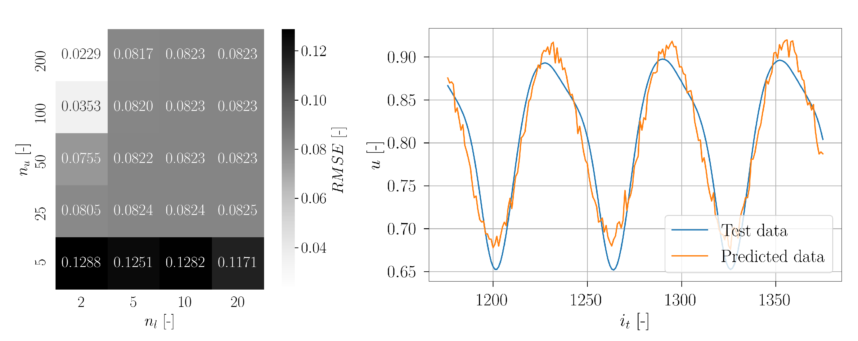
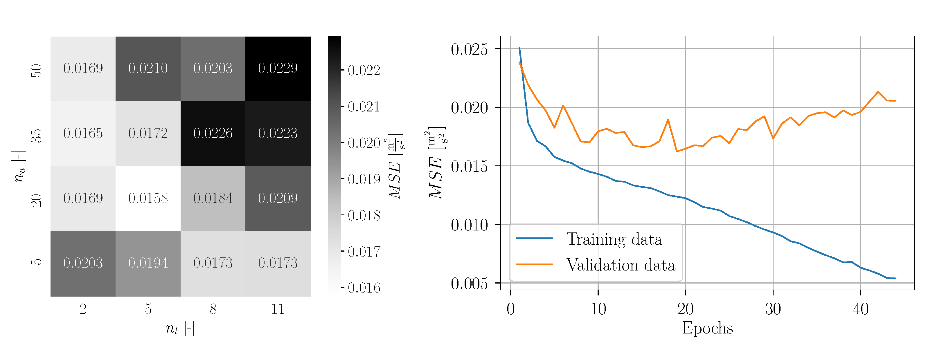
The obtained validation loss values of the grid search with adjusted $n_{in}$ and $n_{out}$ are visualized in Figure 41. A relation can be seen between the number of layers and the resulting prediction accuracy. A high number of Bi-LSTM layers are rather disadvantageous regarding the prediction error. However, too few layers are also not appropriate. A similar dependency is also present regarding the number of Bi-LSTM units per layer. Higher $n_u$ delivers higher prediction errors. Hence, the optimum is located at $n_l=5$ and $n_u=20$. Interestingly, these are the same hyperparameters as obtained for the standard setup.

For the subsequent training with $n_l=5$ and $n_u=20$, the corresponding learning curve is depicted in Figure 41. In contrast to the learning curve of the standard setup, the curve of the training loss is always decreasing, indicating a constant learning progress. The validation loss curve exhibits some noise, but, nonetheless, it can be seen that the validation loss decreases for the first epochs. Around epoch 20, it can be seen that the validation loss begins to increase. The minimum validation loss is obtained at epoch 19. The corresponding Bi-LSTM weights were then saved as the final model. This methodology was chosen to prevent overfitting in the setup.

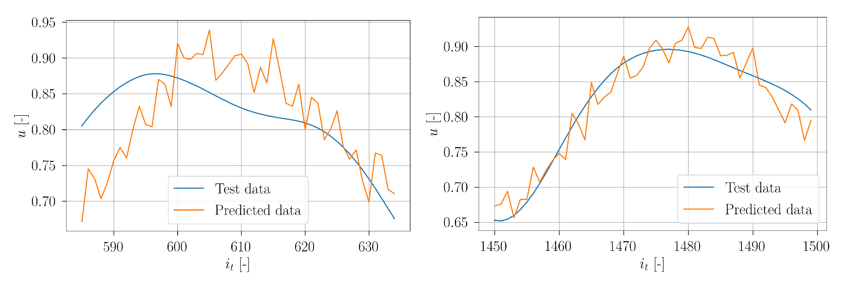
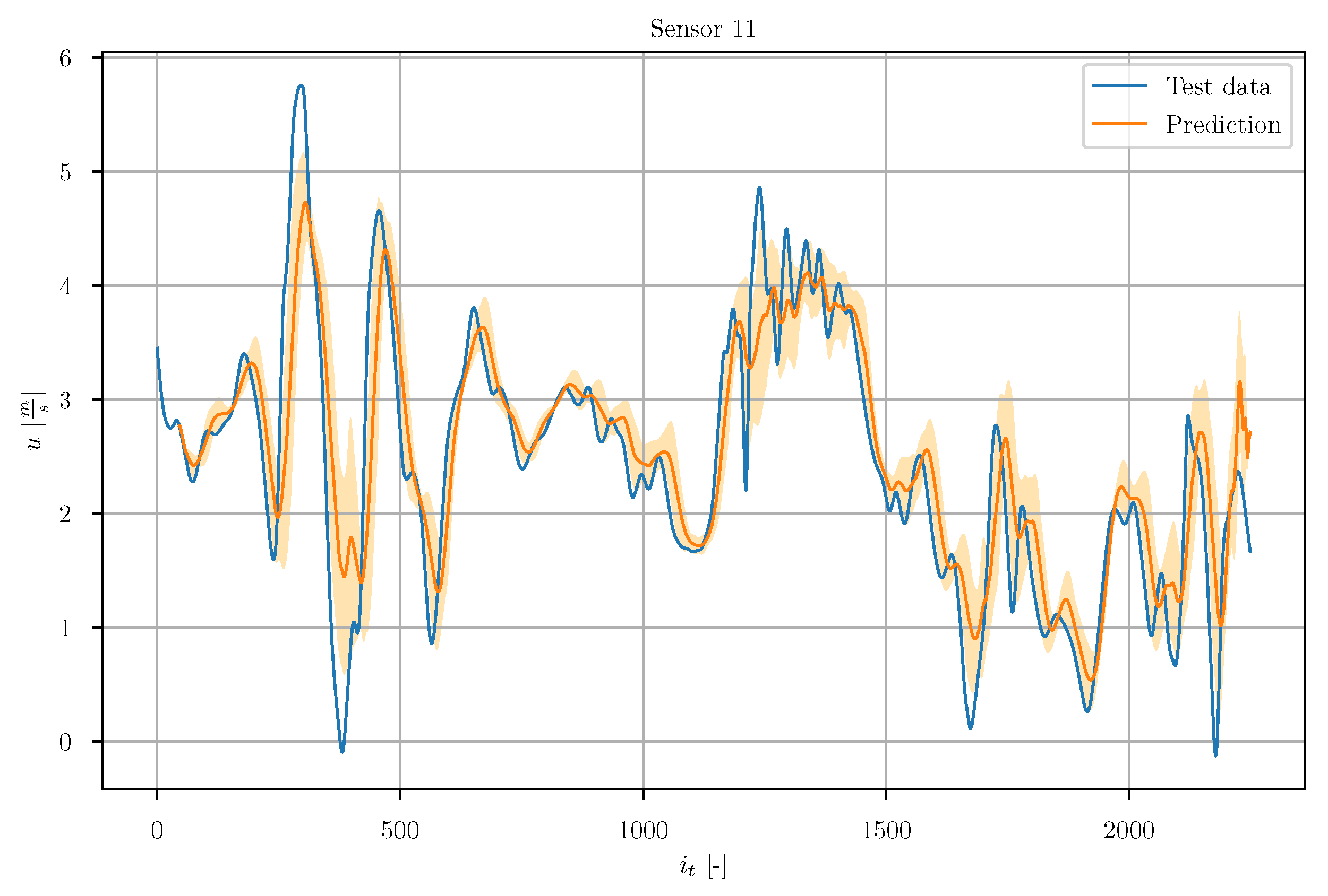
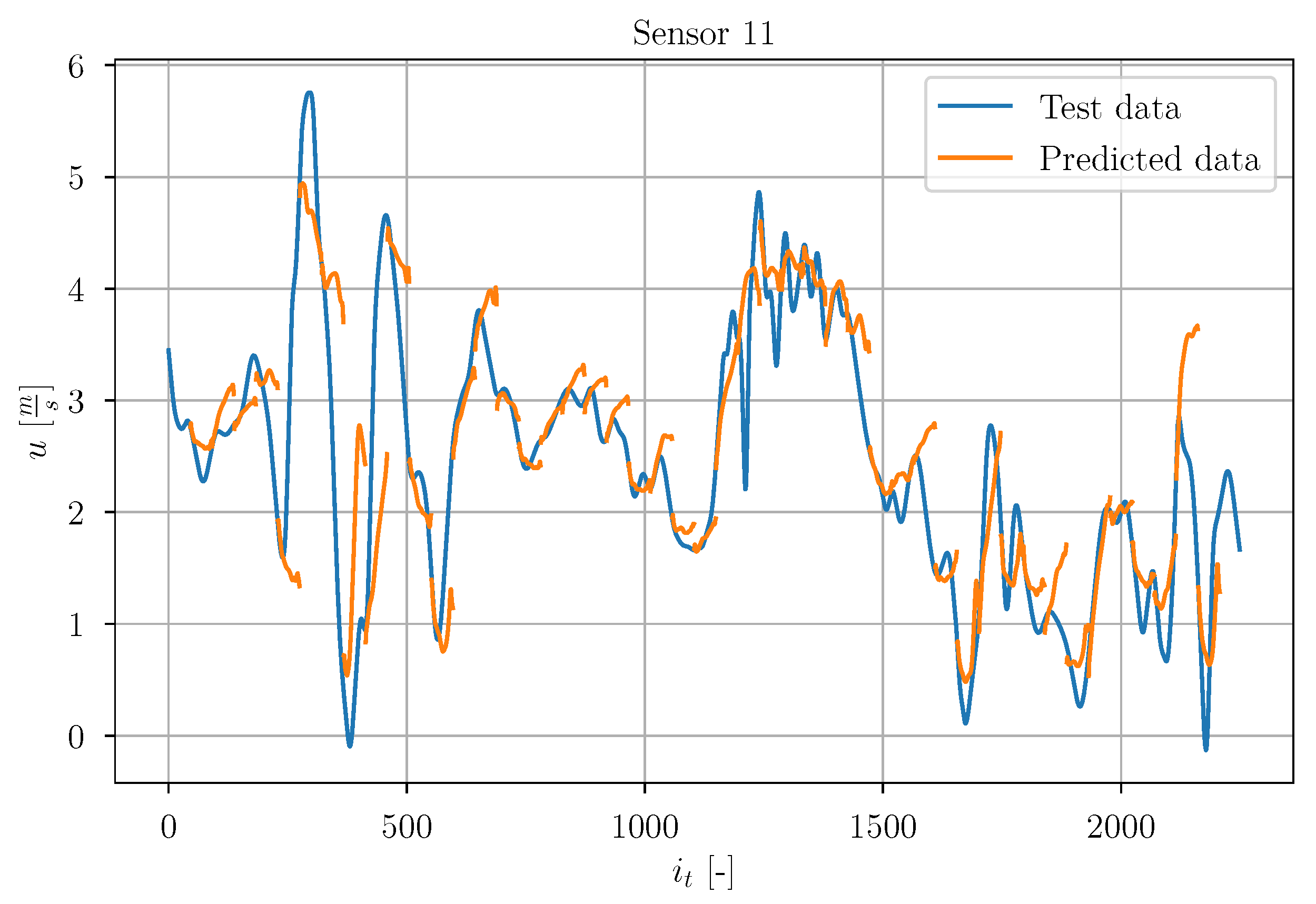
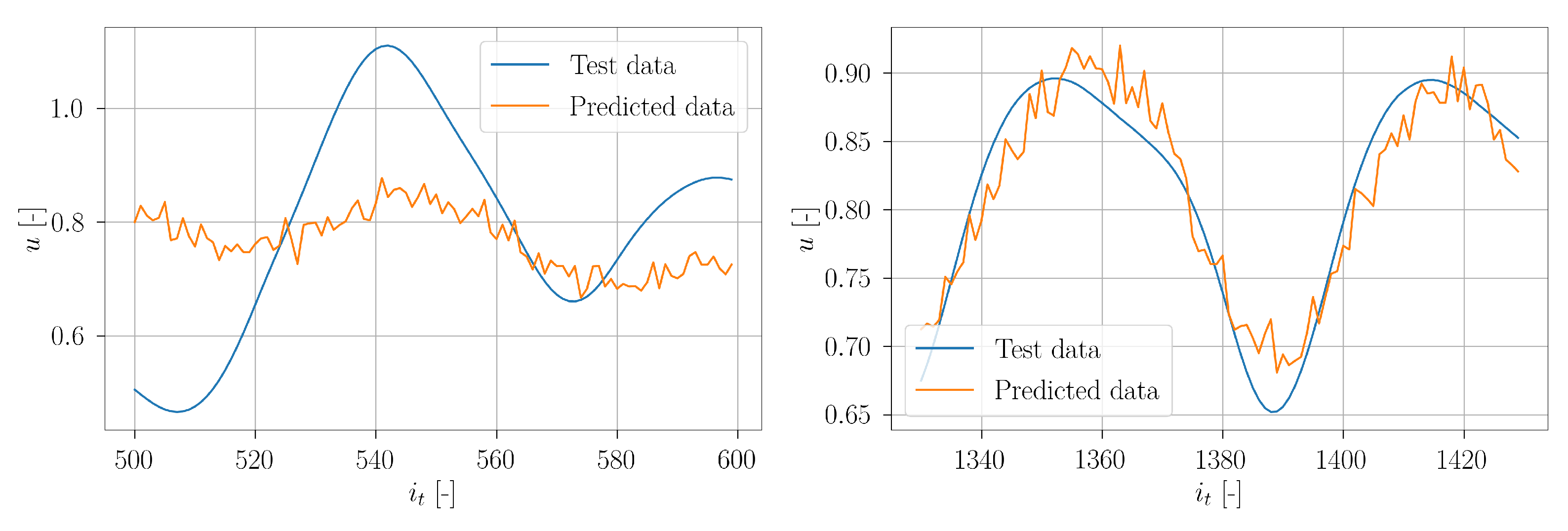
In Figure 42, a set of chronologically consecutive predicted timeseries are depicted together with the true test timeseries of sensor 11. The visualization of these exemplary predictions shows the adjustment of the window width based on the autocorrelation algorithm. It can be seen that the overall accuracy has increased compared to the standard setup. In contrast to the standard setup, here the predicted timeseries do not strive towards a common value. Instead, they coincide rather with the progression of the true signal.

In Figure 43, the averaged timeseries are shown. The prediction results are significantly better compared to the standard setup. The predicted signal shows a significantly better agreement with the true signal. It can be seen that the uncertainty of the prediction, indicated by the orange area around the prediction curve, significantly decreases compared to the standard setup.

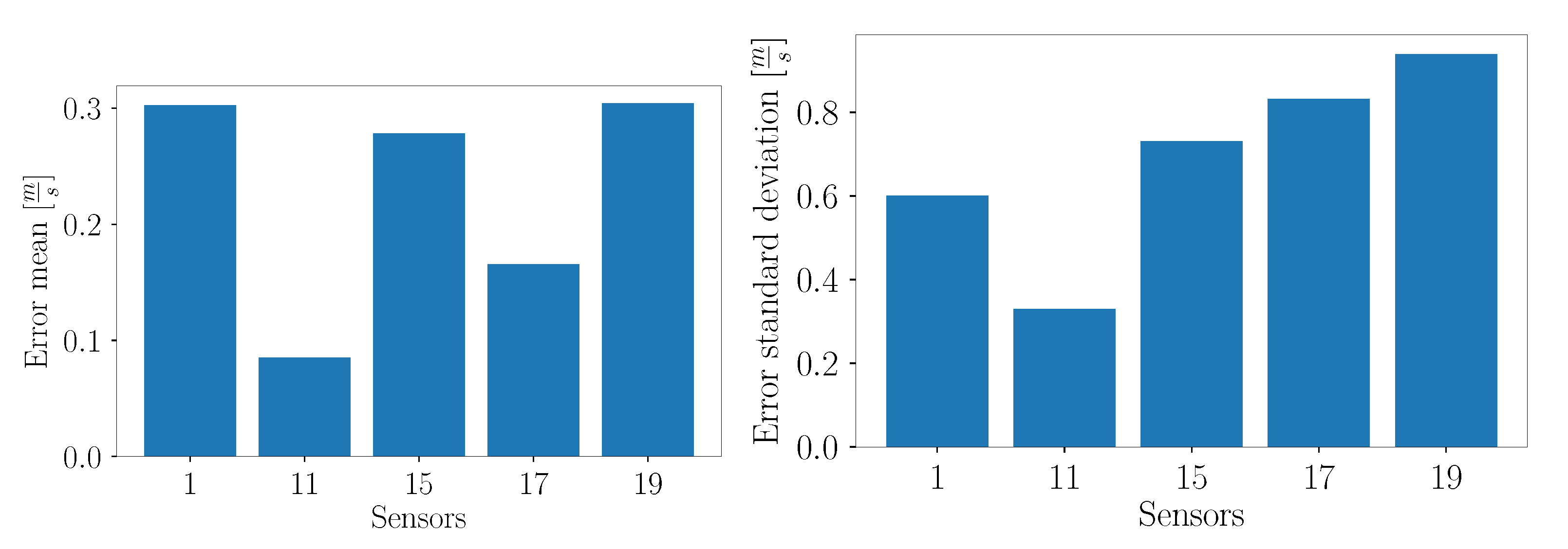
The distribution of the mean error and error standard deviation of each test sensor in Figure 44 shows a similar relation between the sensors as observed for the standard setup. However, for this setup, the mean error of sensor 1 is similar to the values of sensor 15 and 19. Furthermore, the absolute values of the error mean and standard deviation are in general smaller compared to the standard setup, indicating an improvement of the prediction accuracy and a successful prediction of the timeseries.

4. Conclusions and Outlook

In this work, two different flow field data sets were investigated. The first one comprises snapshots of a two-dimensional flow around a cylinder, and the second one comprises snapshots of a fully turbulent flow around a horizontal axis wind turbine. For each data set, a small set of optimally placed sensors was estimated by means of a specific classification-based and reconstruction-based technique, respectively. Subsequently, for the velocity measurement signals obtained from the sensor locations, a data-driven approach for prediction of the velocity component in flow direction was employed. A specific artificial neural network architecture was chosen: stacked bidirectional long short-term memory (Bi-LSTM) networks. For different setups each, a grid search was conducted for hyperparameter optimization. Due to the completely different flow characteristics of the two data sets, different results were obtained. The results of both data sets were compared to each other. The following conclusions can be derived from the paper:

• POD successfully reduce the dimensionality of the flow field data both for cylinder and wind turbine cases.
• SSPOC is sufficient for the cylinder case. On the other hand, this approach is not successful for the complex wind turbine case.
• SSPOR demonstrates its potential for the complex wind turbine case.
• The wake timeseries prediction of the cylinder case shows a good accuracy for the periodic signal, but the transient effects are not predicted accurately.
• The wake prediction of the wind turbine case shows a good accuracy by adjusting the prediction horizon based on evaluation of the autocorrelation function of the timeseries.

For subsequent works, several further approaches can be proposed. In this work, only the prediction of the velocity component in longitudinal direction was considered. The extension of the prediction task to all three velocity components can be proposed. Another interesting aspect could be the reconstruction of the vertical wind profile at discrete horizontal locations based on the predicted velocities at the sensor locations. The reconstruction of the entire flow field is also conceivable. It seems logical that sensors located in the near ground region are more economical because they do not require high and expensive met masts installations. Hence, a further proposal is the investigation of wake prediction based on locally restricted optimal sensor placement. In the case of availability of larger data sets and sufficient computational resources, the approaches for velocity prediction proposed in this work can be enhanced regarding larger Bi-LSTM networks, presumably enabling larger prediction horizons and better prediction accuracy. It is recommended to consider the components of the fluctuating velocity as well as the total velocity components to investigate in which case better prediction accuracy can be achieved.

References

1. Vermeer, L.; Sørensen, J.N.; Crespo, A. Wind turbine wake aerodynamics. Prog. Aerosp. Sci. 2003, 39, 467–510. [Google Scholar] [CrossRef]
2. Sanderse, B.; Van der Pijl, S.; Koren, B. Review of computational fluid dynamics for wind turbine wake aerodynamics. Wind Energy 2011, 14, 799–819. [Google Scholar] [CrossRef] [Green Version]
3. Sun, H.; Gao, X.; Yang, H. A review of full-scale wind-field measurements of the wind-turbine wake effect and a measurement of the wake-interaction effect. Renew. Sustain. Energy Rev. 2020, 132, 110042. [Google Scholar] [CrossRef]
4. Dou, B.; Guala, M.; Lei, L.; Zeng, P. Experimental investigation of the performance and wake effect of a small-scale wind turbine in a wind tunnel. Energy 2019, 166, 819–833. [Google Scholar] [CrossRef]
5. Berger, F.; Kühn, M. Experimental investigation of dynamic inflow effects with a scaled wind turbine in a controlled wind tunnel environment. J. Phys. Conf. Ser. 2018, 1037, 052017. [Google Scholar] [CrossRef] [Green Version]
6. Sun, C.; Tian, T.; Zhu, X.; Hua, O.; Du, Z. Investigation of the near wake of a horizontal-axis wind turbine model by dynamic mode decomposition. Energy 2021, 227, 120418. [Google Scholar] [CrossRef]
7. Churchfield, M.J.; Li, Y.; Moriarty, P.J. A large-eddy simulation study of wake propagation and power production in an array of tidal-current turbines. Philos. Trans. R. Soc. A Math. Phys. Eng. Sci. 2013, 371, 20120421. [Google Scholar] [CrossRef] [Green Version]
8. Kim, Y.; Jost, E.; Bangga, G.; Weihing, P.; Lutz, T. Effects of ambient turbulence on the near wake of a wind turbine. J. Phys. Conf. Ser. 2016, 753, 032047. [Google Scholar] [CrossRef] [Green Version]
9. Jimenez, A.; Crespo, A.; Migoya, E.; García, J. Advances in large-eddy simulation of a wind turbine wake. J. Phys. Conf. Ser. 2007, 75, 012041. [Google Scholar] [CrossRef]
10. Bangga, G.; Lutz, T. Aerodynamic modeling of wind turbine loads exposed to turbulent inflow and validation with experimental data. Energy 2021, 223, 120076. [Google Scholar] [CrossRef]
11. Bastankhah, M.; Porté-Agel, F. A new analytical model for wind-turbine wakes. Renew. Energy 2014, 70, 116–123. [Google Scholar] [CrossRef]
12. Bangga, G.; Hutani, S.; Heramarwan, H. The Effects of Airfoil Thickness on Dynamic Stall Characteristics of High-Solidity Vertical Axis Wind Turbines. Adv. Theory Simul. 2021, 4, 2000204. [Google Scholar] [CrossRef]
13. Ali, N.; Calaf, M.; Cal, R.B. Clustering sparse sensor placement identification and deep learning based forecasting for wind turbine wakes. J. Renew. Sustain. Energy 2021, 13, 023307. [Google Scholar] [CrossRef]
14. Bangga, G.; Guma, G.; Lutz, T.; Krämer, E. Numerical simulations of a large offshore wind turbine exposed to turbulent inflow conditions. Wind Energy 2018, 42, 88–96. [Google Scholar] [CrossRef]
15. Bangga, G.; Lutz, T.; Arnold, M. An improved second-order dynamic stall model for wind turbine airfoils. Wind Energy Sci. 2020, 5, 1037–1058. [Google Scholar] [CrossRef]
16. Kaiser, E.; Noack, B.R.; Cordier, L.; Spohn, A.; Segond, M.; Abel, M.; Daviller, G.; Östh, J.; Krajnović, S.; Niven, R.K. Cluster-based reduced-order modelling of a mixing layer. J. Fluid Mech. 2014, 754, 365–414. [Google Scholar] [CrossRef] [Green Version]
17. Brunton, B.W.; Brunton, S.L.; Proctor, J.L.; Kutz, J.N. Sparse Sensor Placement Optimization for Classification. SIAM J. Appl. Math. 2016, 76, 2099–2122. [Google Scholar] [CrossRef]
18. Manohar, K.; Brunton, B.W.; Kutz, J.N.; Brunton, S.L. Data-driven sparse sensor placement for reconstruction: Demonstrating the benefits of exploiting known patterns. IEEE Control Syst. Mag. 2018, 38, 63–86. [Google Scholar]
19. Salehinejad, H.; Sankar, S.; Barfett, J.; Colak, E.; Valaee, S. Recent Advances in Recurrent Neural Networks. arXiv 2017, arXiv:1801.01078. [Google Scholar]
20. Iungo, G.V.; Santoni-Ortiz, C.; Abkar, M.; Porté-Agel, F.; Rotea, M.A.; Leonardi, S. Data-driven reduced order model for prediction of wind turbine wakes. J. Phys. Conf. Ser. 2015, 625, 012009. [Google Scholar] [CrossRef]
21. Neshat, M.; Nezhad, M.M.; Abbasnejad, E.; Mirjalili, S.; Groppi, D.; Heydari, A.; Tjernberg, L.B.; Garcia, D.A.; Alexander, B.; Shi, Q.; et al. Wind turbine power output prediction using a new hybrid neuro-evolutionary method. Energy 2021, 229, 120617. [Google Scholar] [CrossRef]
22. Xiang, L.; Wang, P.; Yang, X.; Hu, A.; Su, H. Fault detection of wind turbine based on SCADA data analysis using CNN and LSTM with attention mechanism. Measurement 2021, 175, 109094. [Google Scholar] [CrossRef]
23. Chen, H.; Liu, H.; Chu, X.; Liu, Q.; Xue, D. Anomaly detection and critical SCADA parameters identification for wind turbines based on LSTM-AE neural network. Renew. Energy 2021, 172, 829–840. [Google Scholar] [CrossRef]
24. D’Agostino, D.; Andre, M.; Bardet, P.; Serani, A.; Felli, M.; Diez, M. Observing PIV Measurements Through the Lens of Data Clustering. In Proceedings of the 33rd Symposium on Naval Hydrodynamics, Osaka, Japan, 18–23 October 2020. [Google Scholar]
25. D’Agostino, D.; Serani, A.; Stern, F.; Diez, M. Recurrent-type neural networks for real-time short-term prediction of ship motions in high sea state. arXiv 2021, arXiv:2105.13102. [Google Scholar] [CrossRef]
26. Graves, A.; Schmidhuber, J. Framewise phoneme classification with bidirectional LSTM and other neural network architectures. Neural Netw. 2005, 18, 602–610. [Google Scholar] [CrossRef]
27. Huang, X.; Li, Q.; Tai, Y.; Chen, Z.; Liu, J.; Shi, J.; Liu, W. Time series forecasting for hourly photovoltaic power using conditional generative adversarial network and Bi-LSTM. Energy 2022, 246, 123403. [Google Scholar] [CrossRef]
28. Vo, A.H.; Nguyen, T.; Le, T. Brent oil price prediction using Bi-LSTM network. Intell. Autom. Soft Comput. 2020, 26, 1307–1317. [Google Scholar] [CrossRef]
29. Le, T.; Vo, M.T.; Vo, B.; Hwang, E.; Rho, S.; Baik, S.W. Improving electric energy consumption prediction using CNN and Bi-LSTM. Appl. Sci. 2019, 9, 4237. [Google Scholar] [CrossRef] [Green Version]
30. Kocoglu, Y.; Gorell, S.; McElroy, P. Application of Bayesian Optimized Deep Bi-LSTM Neural Networks for Production Forecasting of Gas Wells in Unconventional Shale Gas Reservoirs. In Proceedings of the Unconventional Resources Technology Conference, Houston, TX, USA, 26–28 July 2021; pp. 2176–2196. [Google Scholar]
31. Zürich, C.G.L.E. Data. Available online: https://cgl.ethz.ch/research/visualization/data.php (accessed on 29 October 2021).
32. Günther, T.; Gross, M.; Theisel, H. Generic Objective Vortices for Flow Visualization. ACM Trans. Graph. 2017, 36, 1–11. [Google Scholar] [CrossRef]
33. Popinet, S. Free Computational Fluid Dynamics. ClusterWorld 2004, 2, 7. [Google Scholar]
34. Schepers, J.; Boorsma, K.; A Madsen, H.; Pirrung, G.; Bangga, G.; Guma, G.; Lutz, T.; Potentier, T.; Braud, C.; Guilmineau, E.; et al. IEA Wind TCP Task 29, Phase IV: Detailed Aerodynamics of Wind Turbines; Technical Report; International Energy Agency: Paris, France, 2021. [Google Scholar]
35. Kroll, N.; Rossow, C.C.; Becker, K.; Thiele, F. The MEGAFLOW project. Aerosp. Sci. Technol. 2000, 4, 223–237. [Google Scholar] [CrossRef]
36. Weihing, P.; Letzgus, J.; Bangga, G.; Lutz, T.; Krämer, E. Hybrid RANS/LES capabilities of the flow solver FLOWer—Application to flow around wind turbines. In Proceedings of the Symposium on Hybrid RANS-LES Methods, Strasbourg, France, 26–28 September 2016; Springer: Berlin/Heidelberg, Germany, 2016; pp. 369–380. [Google Scholar]
37. Jameson, A.; Schmidt, W.; Turkel, E. Numerical solution of the Euler equations by finite volume methods using Runge Kutta time stepping schemes. In Proceedings of the 14th Fluid and Plasma Dynamics Conference, Palo Alto, CA, USA, 23–25 June 1981. [Google Scholar]
38. Jiang, G.S.; Shu, C.W. Efficient implementation of weighted ENO schemes. J. Comput. Phys. 1996, 126, 202–228. [Google Scholar] [CrossRef] [Green Version]
39. Troldborg, N.; Sørensen, J.N.; Mikkelsen, R.; Sørensen, N.N. A simple atmospheric boundary layer model applied to large eddy simulations of wind turbine wakes. Wind Energy 2014, 17, 657–669. [Google Scholar] [CrossRef]
40. Developers, G. k-Means Advantages and Disadvantages. Available online: https://developers.google.com/machine-learning/clustering/algorithm/advantages-disadvantages (accessed on 14 December 2021).
41. Belson, B.A.; Tu, J.; Rowley, C.W. Algorithm 945: Modred—A Parallelized Model Reduction Library. ACM Trans. Math. Softw. 2014, 40, 1–23. [Google Scholar] [CrossRef]
42. Taira, K.; Brunton, S.L.; Dawson, S.T.M.; Rowley, C.W.; Colonius, T.; McKeon, B.J.; Schmidt, O.T.; Gordeyev, S.; Theofilis, V.; Ukeiley, L.S. Modal Analysis of Fluid Flows: An Overview. AIAA J. 2017, 55, 4013–4041. [Google Scholar] [CrossRef] [Green Version]
43. Pedregosa, F.; Varoquaux, G.; Gramfort, A.; Michel, V.; Thirion, B.; Grisel, O.; Blondel, M.; Prettenhofer, P.; Weiss, R.; Dubourg, V.; et al. Scikit-learn: Machine Learning in Python. J. Mach. Learn. Res. 2011, 12, 2825–2830. [Google Scholar]
44. de Silva, B.M.; Manohar, K.; Clark, E.; Brunton, B.W.; Kutz, J.N.; Brunton, S.L. PySensors: A Python package for sparse sensor placement. J. Open Source Softw. 2021, 6, 2828. [Google Scholar] [CrossRef]
45. Chollet, F. Keras. Available online: https://keras.io (accessed on 12 January 2022).
46. Abadi, M.; Agarwal, A.; Barham, P.; Brevdo, E.; Chen, Z.; Citro, C.; Corrado, G.S.; Davis, A.; Dean, J.; Devin, M.; et al. TensorFlow: Large-Scale Machine Learning on Heterogeneous Systems. Available online: https://www.tensorflow.org/ (accessed on 12 January 2022).
47. Brownlee, J. Techniques to Handle Very Long Sequences with LSTMs. Available online: https://machinelearningmastery.com/handle-long-sequences-long-short-term-memory-recurrent-neural-networks/ (accessed on 21 December 2021).
48. Brownlee, J. How to Convert a Time Series to a Supervised Learning Problem in Python. Available online: https://machinelearningmastery.com/convert-time-series-supervised-learning-problem-python/ (accessed on 3 July 2021).
49. Brownlee, J. How to use Learning Curves to Diagnose Machine Learning Model Performance. Available online: https://machinelearningmastery.com/learning-curves-for-diagnosing-machine-learning-model-performance/ (accessed on 2 January 2022).
50. Dancho, M. Time Series Analysis: KERAS LSTM, Deep Learning - Part 1. Available online: https://www.business-science.io/timeseries-analysis/2018/04/18/keras-lstm-sunspots-time-series-prediction.html (accessed on 10 January 2022).
51. Seabold, S.; Perktold, J. Statsmodels: Econometric and Statistical Modeling with Python. In Proceedings of the 9th Python in Science Conference, Austin, TX, USA, 28 June–3 July 2010. [Google Scholar]
52. Weiss, J. A Tutorial on the Proper Orthogonal Decomposition. American Institute of Aeronautics and Astronautics. 2019, p. AIAA 2019–3333. Available online: https://depositonce.tu-berlin.de/handle/11303/9456 (accessed on 12 January 2022).
53. Goodfellow, I.; Bengio, Y.; Courville, A. Deep Learning; MIT Press: Cambridge, MA, USA, 2016; Available online: http://www.deeplearningbook.org (accessed on 12 January 2022).
54. Tian, X.; Zhang, J.; Ma, Z.; He, Y.; Wei, J.; Wu, P.; Situ, W.; Li, S.; Zhang, Y. Deep LSTM for Large Vocabulary Continuous Speech Recognition. arXiv 2017, arXiv:1703.07090. [Google Scholar]
55. Bellman, R. Dynamic Programming; Princeton University Press: Princeton, NJ, USA, 1957. [Google Scholar]
56. VanderPlas, J. In Depth: Gaussian Mixture Models. Available online: https://jakevdp.github.io/PythonDataScienceHandbook/05.12-gaussian-mixtures.html (accessed on 20 December 2021).
57. Frost, J. Autocorrelation and Partial Autocorrelation in Time Series Data. Available online: https://statisticsbyjim.com/time-series/autocorrelation-partial-autocorrelation/ (accessed on 3 January 2022).
Short Biography of Authors
Energies 15 03773 i001MSc. Martin Geibel completed his master degree in Aerospace Engineering from the University of Stuttgart in 2022. His research interests are in aerodynamics, wind energy and machine learning. He has collected some industrial experiences from different places including MartinMechanic Friedrich Martin GmbH & Co KG, DUROtherm Kunststoffverarbeitung GmbH, HÄNDLE Härterei GmbH & Co. KG and MAHLE International GmbH. He loves making music, especially playing guitar and piano, as well as doing some sports (strength training and running).
Energies 15 03773 i002Dr. Galih Bangga has collected years of experience in the aerodynamics of wind turbine as a scientist at the University of Stuttgart. During this period of time, he was involved in numerous projects in close cooperation with industry, universities and research institutions. He continuously provides supports in academic community by serving as editors and reviewers in technical journals and is currently active as a member in a technical committee within EAWE (European Academy of Wind Energy). He joined DNV from 2021 as a senior developer of an industry standard wind turbine design tool focusing in its aerodynamic models development. In his free time, he loves to visit cafes, to learn about coffee-making process and to do some latte arts.
Figure 1. Flow field in the wake of cylinder during the periodic quasi steady state.
Energies 15 03773 g001
Figure 2. Flow field in the wake of a rotating wind turbine showing the complex characteristics of the flow interactions.
Energies 15 03773 g002
Figure 3. Vertically placed measurement points (white rhombuses) used for error estimation. Snapshot at i t = 0 in the background.
Energies 15 03773 g003
Figure 4. Stacked Bi-LSTM structure adopted in the present studies.
Energies 15 03773 g004
Figure 5. Training sensors (green) and test sensors (red) with snapshot at i t = 0 as background.
Energies 15 03773 g005
Figure 6. First three POD modes from the cylinder case. Top: 1st mode, middle: 2nd mode, bottom: 3rd mode.
Energies 15 03773 g006
Figure 7. Temporal coefficients of POD mode 1 and 2 over the snapshot index.
Energies 15 03773 g007
Figure 8. Temporal coefficient of POD mode 3 over the snapshot index.
Energies 15 03773 g008
Figure 9. Visualization of the cluster transition matrix (CTM). Transition occurs from cluster C k to cluster C j .
Energies 15 03773 g009
Figure 10. Visualization of the number of transitions from cluster C k to cluster C j .
Energies 15 03773 g010
Figure 11. Sensor locations with snapshot at i t = 1500 as background.
Energies 15 03773 g011
Figure 12. True and predicted cluster assignment over the snapshot index i t .
Energies 15 03773 g012
Figure 13. Velocity timeseries at sensor 4 and the considered time ranges. The time intervals from which data was used for training and test data are colored in green and red, respectively. Top: setup 1, middle: setup 2, bottom: setup 3, setup 4 and setup 5.
Energies 15 03773 g013
Figure 14. Heatmap and timeseries reconstruction for setup 1 of the cylinder case.
Energies 15 03773 g014
Figure 15. Heatmap and timeseries reconstruction for setup 2 of the cylinder case.
Energies 15 03773 g015
Figure 16. Heatmap and timeseries reconstruction for setup 3 of the cylinder case.
Energies 15 03773 g016
Figure 17. Timeseries reconstruction for setup 4 of the cylinder case.
Energies 15 03773 g017
Figure 18. Timeseries reconstruction for setup 5 of the cylinder case.
Energies 15 03773 g018
Figure 19. Visualization of three different POD modes of the near wake for the wind turbine case. From top to bottom: mode 1, 5 and 15, respectively.
Energies 15 03773 g019
Figure 20. Contribution of POD modes to the total fluctuation kinetic energy and the cumulative portion of POD modes to the total fluctuation kinetic energy.
Energies 15 03773 g020
Figure 21. Time averaged mean velocity field in the wake of the wind turbine case.
Energies 15 03773 g021
Figure 22. Temporal POD coefficients of mode 1, 5 and 15 over the snapshot index.
Energies 15 03773 g022
Figure 23. Temporal POD coefficient of mode 500 over the snapshot index.
Energies 15 03773 g023
Figure 24. Relation between inertia and k for setup 1 (left) and setup 2 (right).
Energies 15 03773 g024
Figure 25. Counted cluster transitions for setup 2 of the wind turbine case.
Energies 15 03773 g025
Figure 26. Silhouette coefficient over k for hierarchical agglomerative clustering with raw snapshot data in the POD subspace.
Energies 15 03773 g026
Figure 27. Silhouette plot for k = 6 (left) and k = 10 (right) for the hierarchical agglomerative clustering method.
Energies 15 03773 g027
Figure 28. Akaike information criterion (AIC) and Bayesian information criterion (BIC) over k for setup 1.
Energies 15 03773 g028
Figure 29. Visualization of the number of transitions from cluster C k to cluster C j for setup 2.
Energies 15 03773 g029
Figure 30. Assigned cluster C k over i t for setup 2.
Energies 15 03773 g030
Figure 31. Akaike information criterion (AIC) and Bayesian information criterion (BIC) over k for setup 4.
Energies 15 03773 g031
Figure 32. Reconstruction error over the number of used basis modes.
Energies 15 03773 g032
Figure 33. Total mean and variance of true and predicted signals (each averaged over all measurement points and all velocity components) depending on r.
Energies 15 03773 g033
Figure 34. Final set of n s = 20 sensors obtained from SSPOR.
Energies 15 03773 g034
Figure 35. Reconstructed wake field compared against true data for two different time instances.
Energies 15 03773 g035
Figure 36. Visualization of the grid search results (left) and the learning curve of a subsequent training for n l = 5 and n u = 20 (right).
Energies 15 03773 g036
Figure 37. Predicted and true timeseries of sensor 11 for the standard setup. The presented data is discontinuous to illustrate the windows size.
Energies 15 03773 g037
Figure 38. Averaged predicted timeseries and true timeseries of sensor 11 for the standard setup.
Energies 15 03773 g038
Figure 39. Mean and standard deviation of each sensor error for the standard setup.
Energies 15 03773 g039
Figure 40. Autocorrelation function of measured velocity component in x-direction for sensor 11.
Energies 15 03773 g040
Figure 41. Visualization of the grid search results for adjusted n i n and n o u t (left) and the learning curve of a subsequent training for n l = 5 and n u = 20 (right).
Energies 15 03773 g041
Figure 42. Predicted and true timeseries of sensor 11 for adjusted n i n and n o u t . The presented data is discontinuous to illustrate the windows size.
Energies 15 03773 g042
Figure 43. Averaged predicted timeseries and true timeseries of sensor 11 for adjusted n i n and n o u t .
Energies 15 03773 g043
Figure 44. Mean and standard deviation of each sensor error for adjusted n i n and n o u t .
Energies 15 03773 g044