
Computational Optimization of Free-Piston Stirling Engine by Variable-Step Simplified Conjugate Gradient Method with Compatible Strategies


Abstract
:1. Introduction
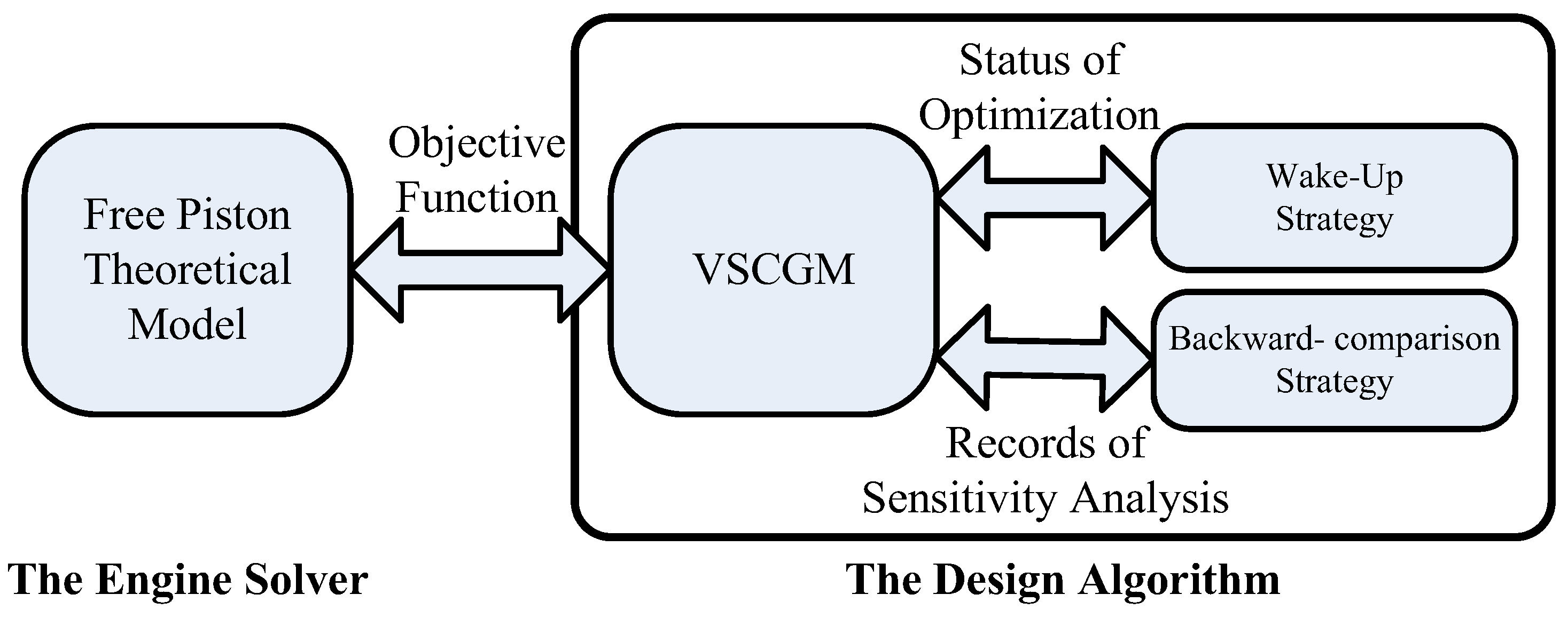
2. Design Algorithm
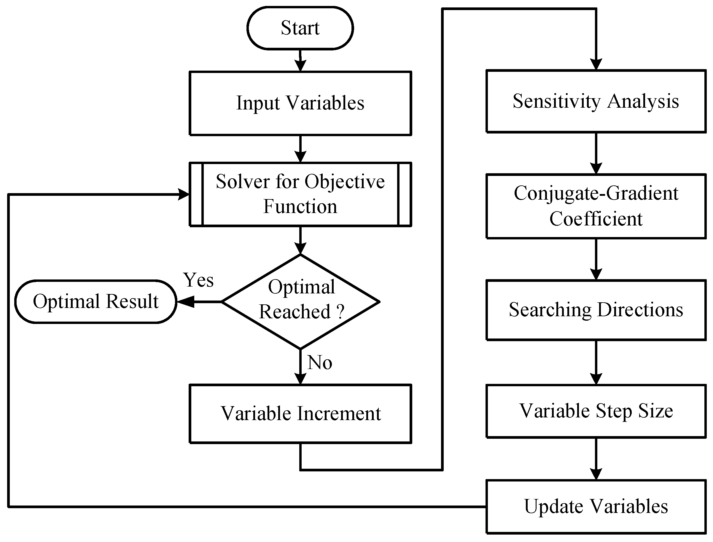
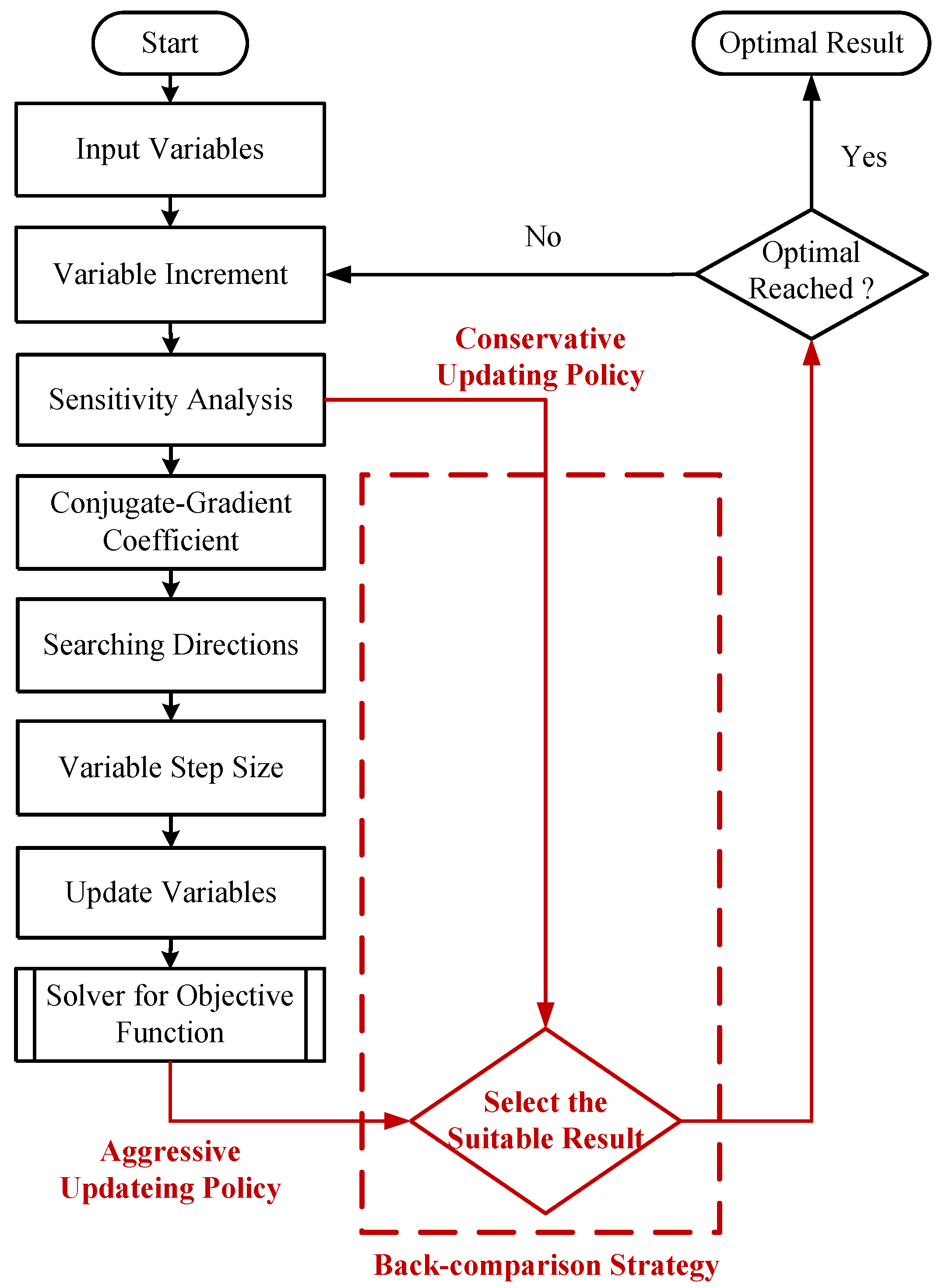
2.1. Variable-Step Simplified Conjugate Gradient Method, VSCGM
- Use Equation (4) for the objective function gradient with the perturbation of each designed variable. Meanwhile, the step size is determined by Equation (5).
- Evaluate the conjugate gradient coefficient by the ratio of the objective function gradients.
- Calculate the searching direction with a linear combination of the objective function gradients and conjugate gradients .
- Update the designed variables in terms of the variable step size and the searching direction .
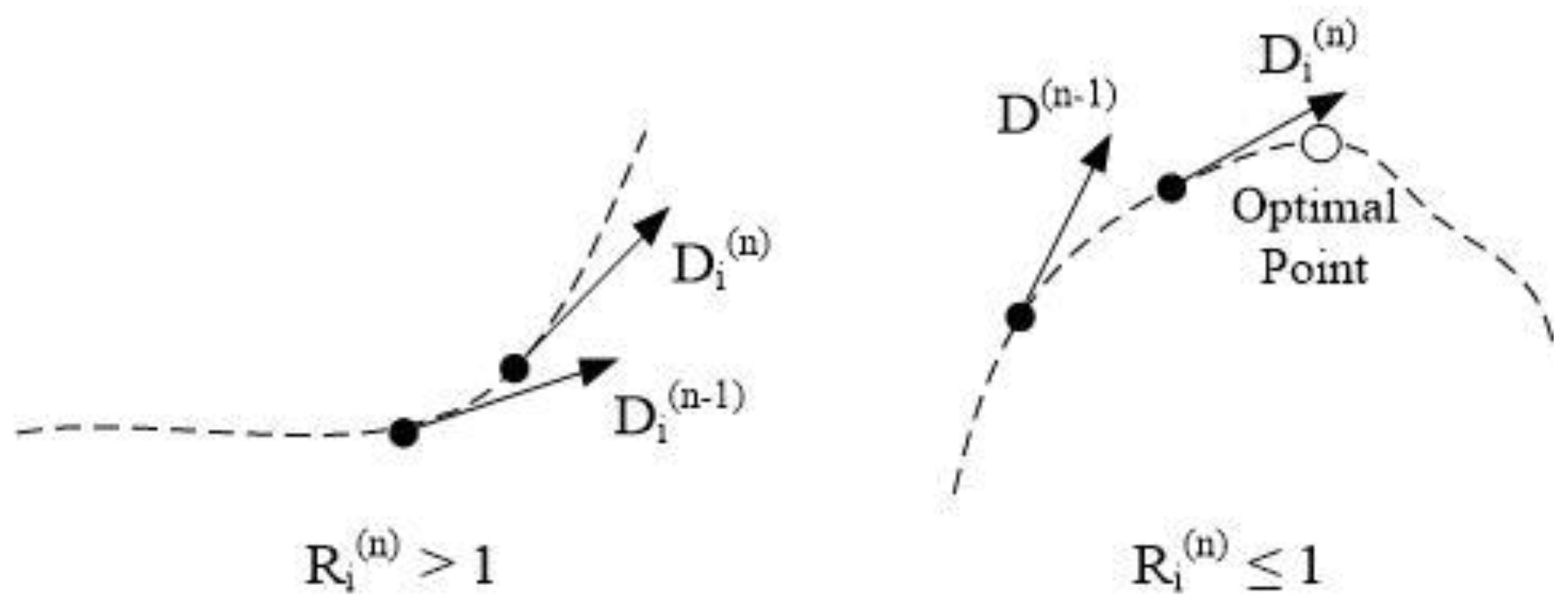
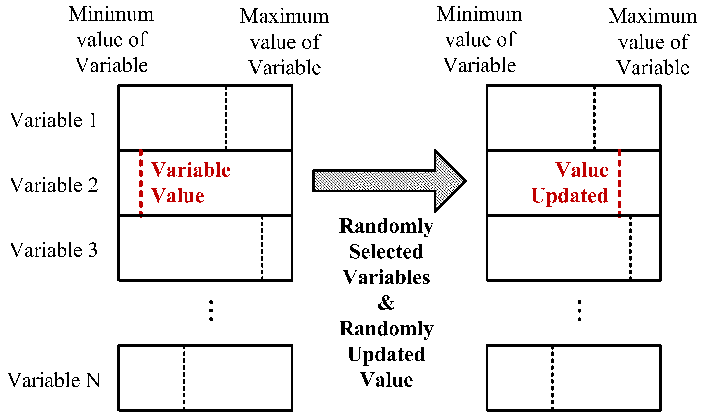
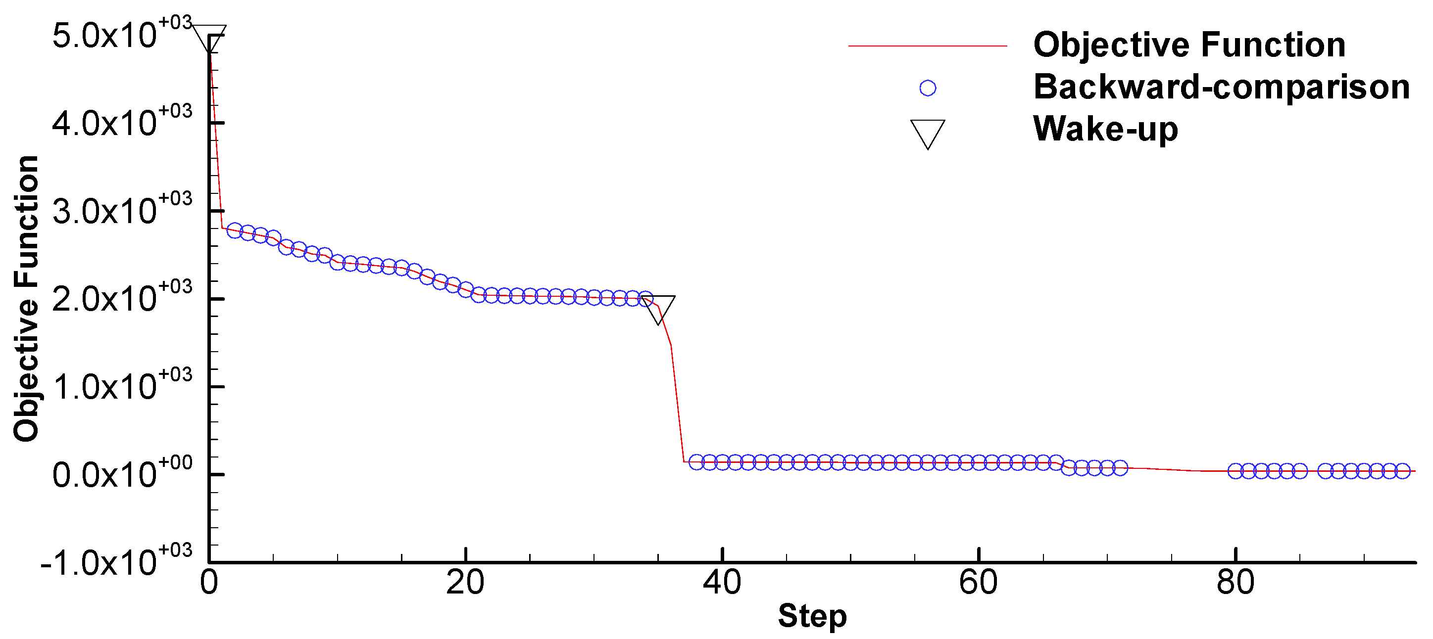
2.2. Wake-Up and Backward-Comparison Strategies
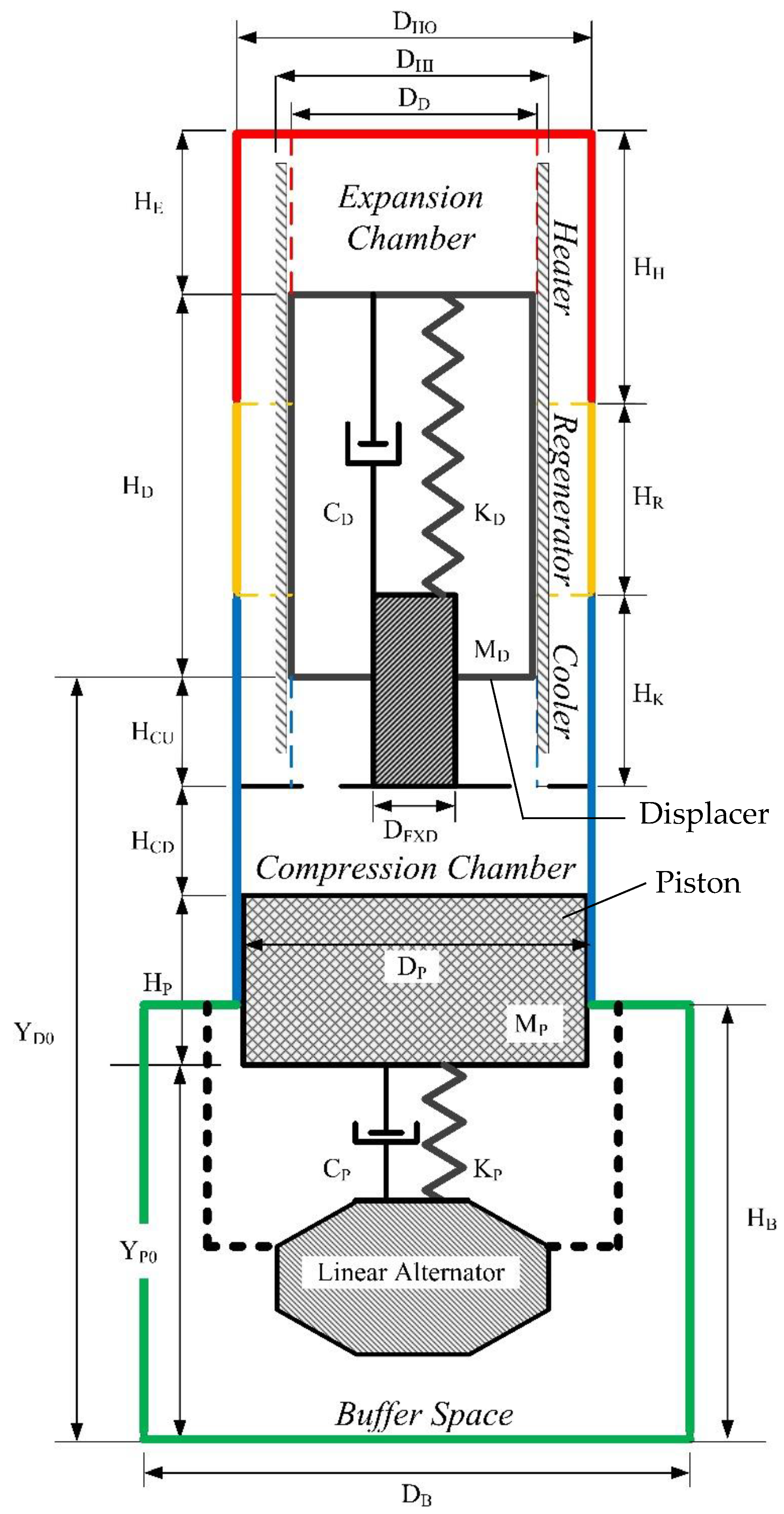
2.3. Theoretical Model of Free-Piston Stirling Engine
3. Test Cases
4. Results and Discussion
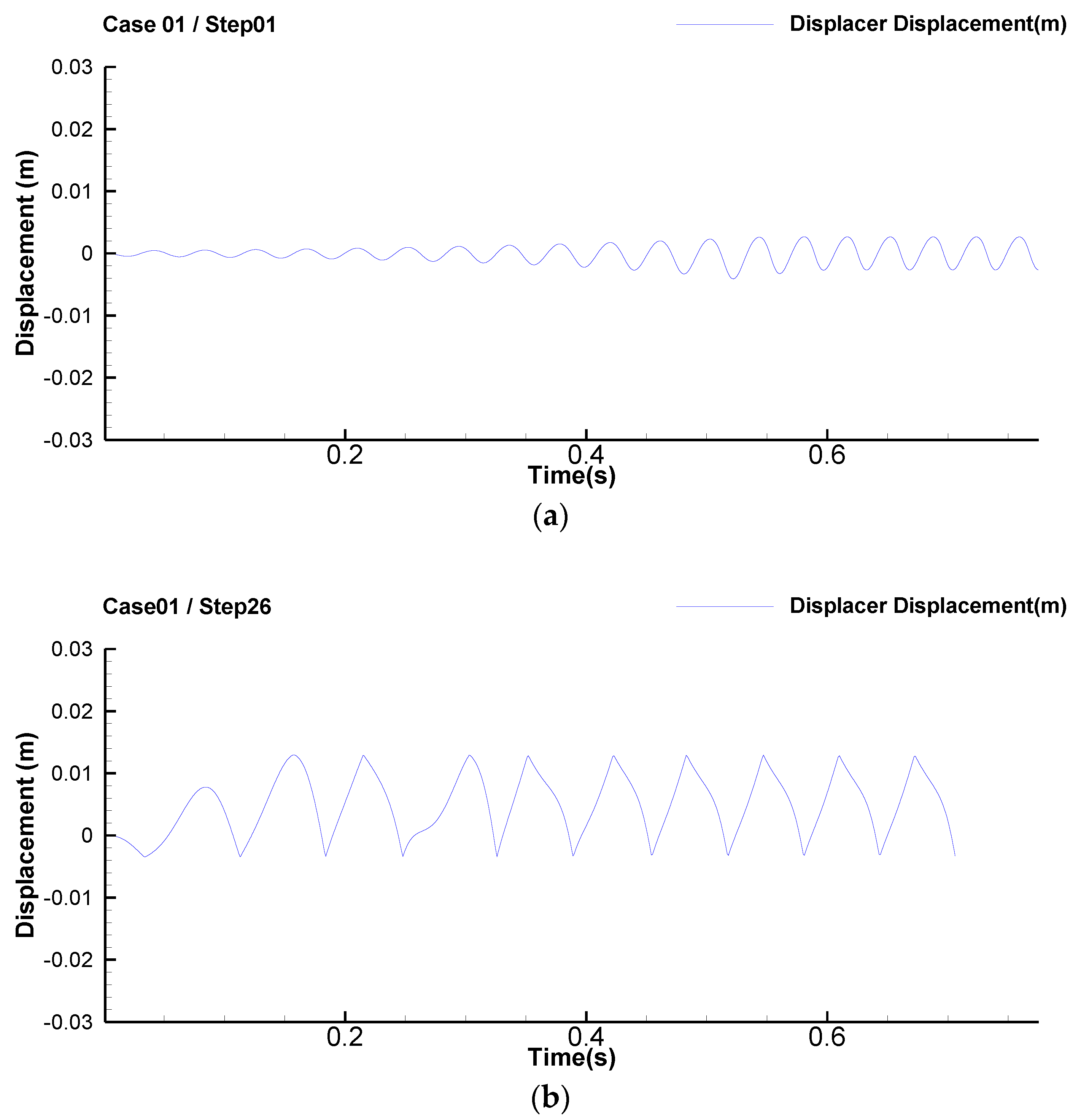
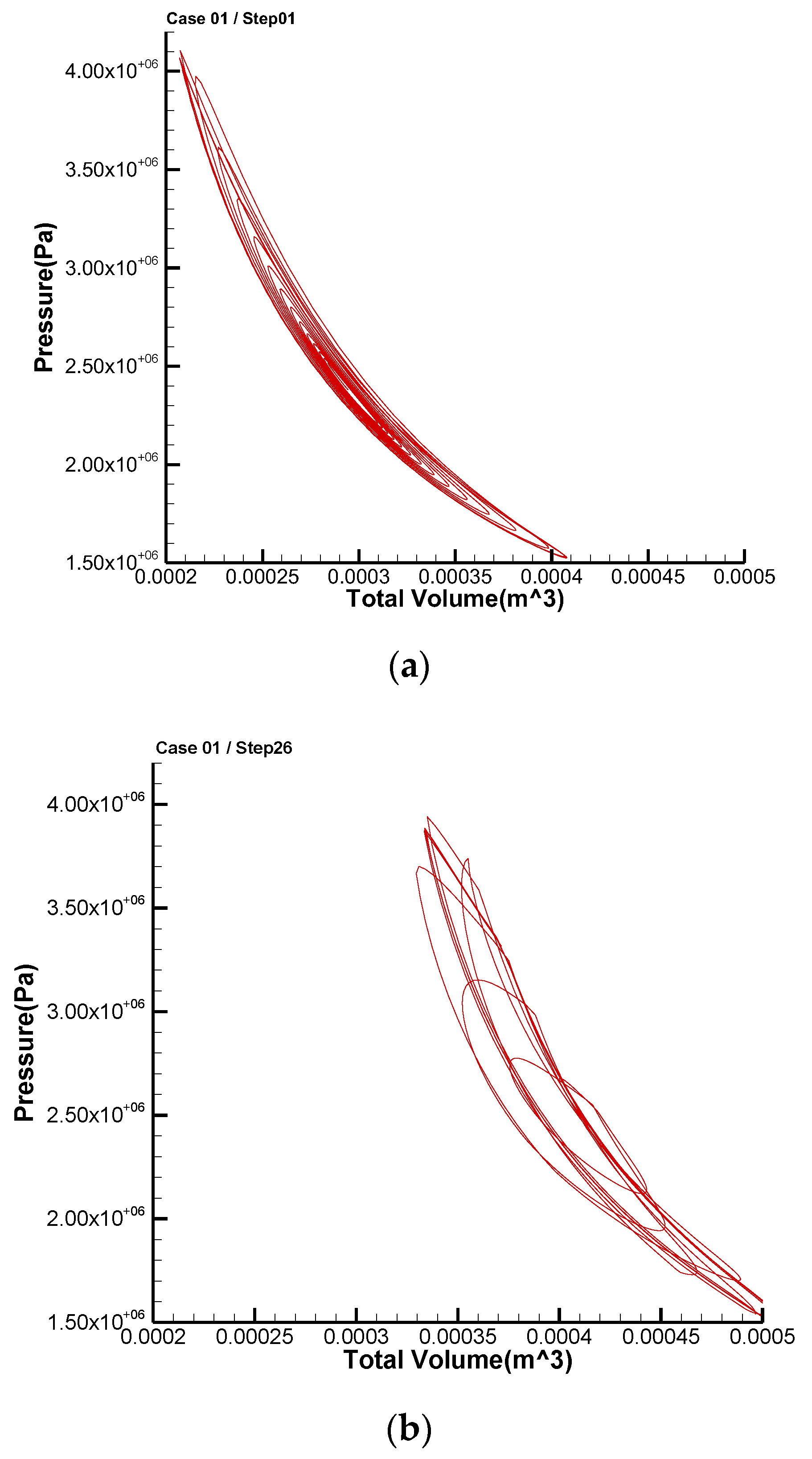
4.1. Case 1 by VSCGM
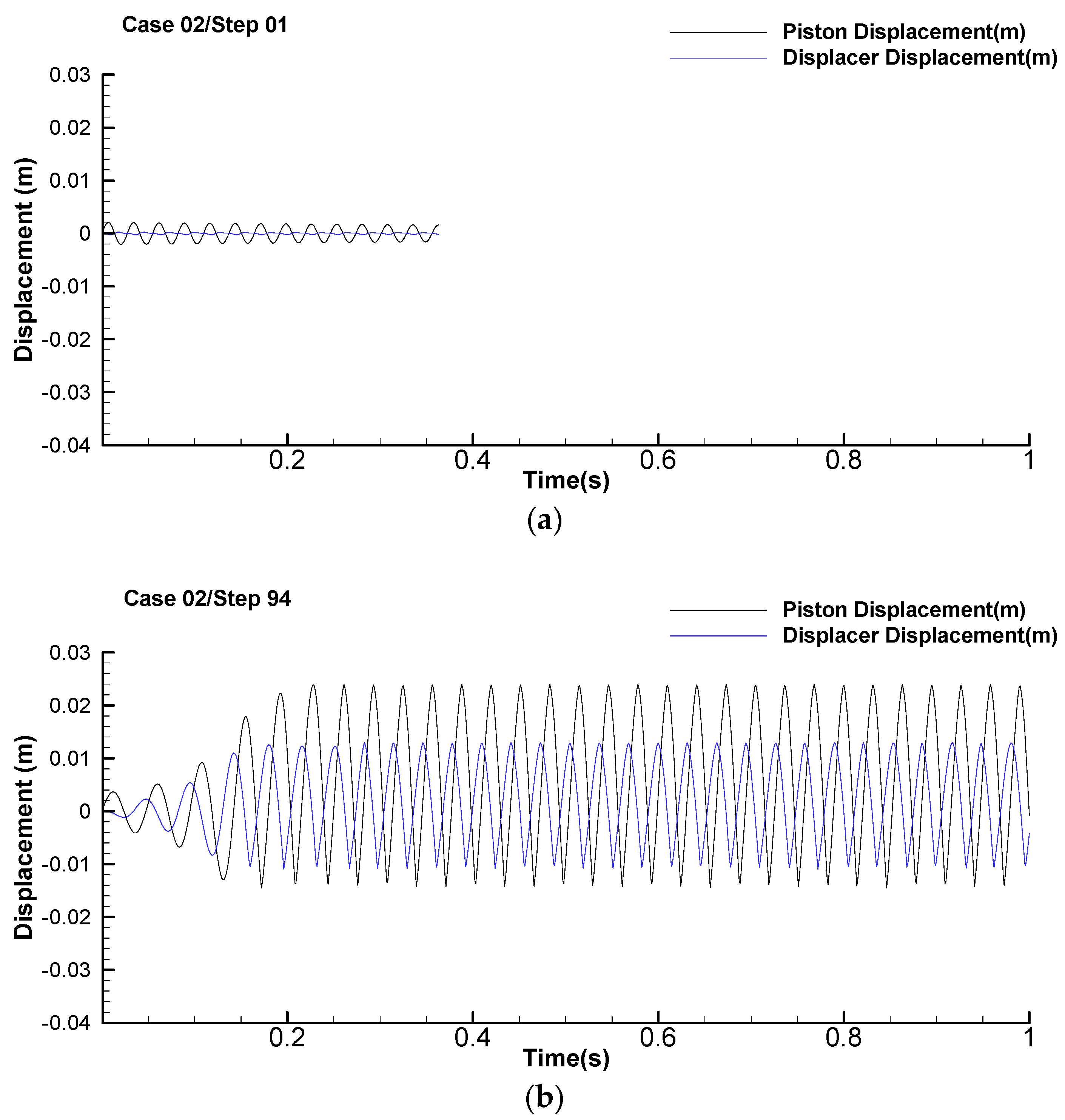
4.2. Case 2 by VSCGM + Wake-Up and Backward-Comparison Strategies
5. Conclusions
Author Contributions
Funding
Conflicts of Interest
Nomenclature
| A | area (m2) |
| C | damping (Ns/m) |
| D | searching direction |
| F | objective function |
| g | gravitational constant (m/s2) |
| G | gain value |
| I | total data number |
| K | stiffness of spring (N/m) |
| M | mass (kg) |
| P | pressure (Pa) |
| R | the ratio of searching direction |
| s | stroke (m) |
| S | step size for the optimization |
| T | temperature (K) |
| v | iterative values |
| V | volume of chamber (m3) |
| x | designed variable |
| ΔX | perturbation of designed variable |
| Greek symbols | |
| conjugate gradient coefficient | |
| Superscripts | |
| n | number of iteration |
| Subscripts | |
| B | back pressure chamber |
| B0 | initial condition of back pressure chamber |
| C | compression chamber |
| C0 | initial condition of compression chamber |
| D | displacer |
| DB | bottom surface of displacer |
| DU | upper surface of displacer |
| E | expansion chamber |
| E0 | initial condition of expansion chamber |
| H | heater chamber |
| i | index of iterative value |
| K | cooler chamber |
| Max | maximum value |
| min | minimum value |
| P | piston |
| R | regenerator chamber |
| W | working gas |
References
- Finkelstein, T.; Organ, A.J. Air Engines; ASME Press: New York, NY, USA, 2001. [Google Scholar]
- Organ, J. The Regenerator and the Stirling Engine; Mechanical Engineering Publications Limited: London, UK, 1997. [Google Scholar]
- Kongtragool, B.; Wongwises, S. A review of solar-powered Stirling engines and low temperature differential Stirling engines. Renew. Sustain. Energy Rev. 2003, 7, 131–154. [Google Scholar] [CrossRef]
- Walker, G.; Senft, J.R. Free Piston Stirling Engine; Springer: Berlin/Heidelberg, Germany, 1985. [Google Scholar]
- Rogdakis, E.D.; Bormpilas, N.A.; Koniakos, I.K. A Thermodynamic Study for the Optimization of Stable Operation of Free Piston Stirling Engines. Energy Conserv. Manag. 2004, 45, 575–593. [Google Scholar] [CrossRef]
- Zare, S.; Tavakolpour-Saleh, A.R. Frequency-based Design of a Free Piston Engine Using Genetic Algorithm. Energy 2016, 109, 466–480. [Google Scholar] [CrossRef]
- Kuo, S.S. Computer Applications of Numerical Methods; Addison-Wesley Publishing Company: Boston, MA, USA, 1972. [Google Scholar]
- Nocedal, J.; Wright, S.J. Numerical Optimization, 2nd ed.; Springer: New York, NY, USA, 2006; pp. 30–62. [Google Scholar]
- Cheng, C.H.; Chang, M.H. A simplified conjugate-gradient method for shape identification based on thermal data. Numer. Heat Transf. Part B Fundam. 2003, 43, 489–507. [Google Scholar] [CrossRef]
- Cheng, C.H.; Lin, Y.T. Optimization of a Stirling Engine by Variable-Step Simplified Conjugate-Gradient Method and Neural Network Training Algorithm. Energies 2020, 13, 5164. [Google Scholar] [CrossRef]
- Fliege, J.; Svaiter, B. Steepest descent methods for multicriteria optimization. Math. Methods Oper. Res. 2000, 51, 479–797. [Google Scholar] [CrossRef]
- Wedderburn, R.W.M. Quasi-likelihood functions, generalized linear models, and the Gauss—Newton method. Biometrika 1974, 61, 439–447. [Google Scholar]
- Rao, S.S. Engineering Optimization: Theory and Practice; Wiley: Hoboken, NJ, USA, 2009. [Google Scholar]
- Jang, J.Y.; Cheng, C.H.; Huang, Y.X. Optimal design of baffles locations with interdigitated flow channels of a centimeter-scale proton exchange membrane fuel cell. Int. J. Heat Mass Transf. 2010, 53, 732–743. [Google Scholar] [CrossRef]
- Huang, Y.X.; Wang, X.D.; Cheng, C.H.; Lin, D.T.W. Geometry optimization of thermoelectric coolers using simplified conjugate gradient method. Energy 2013, 59, 689–697. [Google Scholar] [CrossRef]
- Cheng, C.H.; Huang, Y.X.; King, S.C.; Lee, C.I.; Leu, C.H. CFD-based optimal design of a micro-reformer by integrating computational fluid dynamics code using a simplified conjugate-gradient method. Energy 2014, 70, 355–365. [Google Scholar] [CrossRef]
- Cheng, C.H.; Le, Q.T.; Huang, J.S. Numerical prediction of performance of a low-temperature-differential gamma-type Stirling engine. Numer. Heat Transf. Part A Appl. 2018, 74, 1770–1785. [Google Scholar] [CrossRef]

| Designed Variables | Initial Design of Case 1 | Initial Design of Case 2 |
|---|---|---|
| Displacer Spring Stiffness (N/m) | 68,700 | 67,691.38 |
| Displacer Mass (kg) | 0.303 | 2.58 |
| Piston Spring Stiffness (N/m) | 27,631 | 28,303.86 |
| Piston Mass (kg) | 2.750 | 13.75 |
| Displacer Diameter (m) | 0.07 | 0.07 |
| Piston Diameter (m) | 0.07 | 0.07 |
| Displacer Height (m) | 0.148 | 0.148 |
| Piston Height (m) | 0.060 | 0.060 |
| Displacer Install Position (m) | 0.197 | 0.19766 |
| Piston Install Position (m) | 0.106 | 0.106 |
| Fixed Variables | Value |
|---|---|
| Charged pressure (bar) | 10 |
| Heating temperature (K) | 900 |
| Cooling temperature (K) | 300 |
| Porosity of regenerator | 0.612 |
| Heater diameter (m) | 0.084 |
| Heater inner fin number | 10 |
| Heater inner fin angle (degree) | 18 |
| Heater height (m) | 0.062 |
| Regenerator diameter (m) | 0.084 |
| Regenerator height (m) | 0.4156 |
| Cooler diameter (m) | 0.084 |
| Cooler inner fin number | 10 |
| Cooler inner fin angle (degree) | 18 |
| Cooler height (m) | 0.065 |
| Lower compression chamber height (m) | 0.2316 |
| Back pressure chamber diameter (m) | 0.13 |
| Back pressure chamber height (m) | 0.106 |
| Variable | Optimal Value |
|---|---|
| Displacer Spring Stiffness (N/m) | 67,783.38 |
| Displacer Mass (kg) | 22.6 |
| Piston Spring Stiffness (N/m) | 29,070.53 |
| Piston Mass (kg) | 34.375 |
| Displacer Diameter (m) | 0.0669 |
| Piston Diameter (m) | 0.0660 |
| Displacer Height (m) | 0.108 |
| Piston Height (m) | 0.0504 |
| Displacer Installation Position (m) | 0.1141 |
| Piston Installation Position (m) | 0.038 |
| Variable | Value |
|---|---|
| Displacer Spring Stiffness (N/m) | 64,969.5 |
| Displacer Mass (kg) | 3.03 |
| Piston Spring Stiffness (N/m) | 27,592.4 |
| Piston Mass (kg) | 5.13 |
| Displacer Diameter (m) | 0.0790 |
| Piston Diameter (m) | 0.0563 |
| Displacer Height (m) | 0.142 |
| Piston Height (m) | 0.069 |
| Displacer Installation Position (m) | 0.200 |
| Piston Installation Position (m) | 0.085 |
| Case | Amplitude (m) | Frequency (Hz) | Power Output (W) |
|---|---|---|---|
| Case 1 (VSCGM) | 0.0164 | 15.849 | 667.775 |
| Case 2 (VSCGM + wake-up and backward-comparison) | 0.0239 | 31.110 | 889.430 |
Publisher’s Note: MDPI stays neutral with regard to jurisdictional claims in published maps and institutional affiliations. |
© 2022 by the authors. Licensee MDPI, Basel, Switzerland. This article is an open access article distributed under the terms and conditions of the Creative Commons Attribution (CC BY) license (https://creativecommons.org/licenses/by/4.0/).
Share and Cite
Cheng, C.-H.; Lin, Y.-T. Computational Optimization of Free-Piston Stirling Engine by Variable-Step Simplified Conjugate Gradient Method with Compatible Strategies. Energies 2022, 15, 3569. https://doi.org/10.3390/en15103569
Cheng C-H, Lin Y-T. Computational Optimization of Free-Piston Stirling Engine by Variable-Step Simplified Conjugate Gradient Method with Compatible Strategies. Energies. 2022; 15(10):3569. https://doi.org/10.3390/en15103569
Chicago/Turabian StyleCheng, Chin-Hsiang, and Yu-Ting Lin. 2022. "Computational Optimization of Free-Piston Stirling Engine by Variable-Step Simplified Conjugate Gradient Method with Compatible Strategies" Energies 15, no. 10: 3569. https://doi.org/10.3390/en15103569
APA StyleCheng, C.-H., & Lin, Y.-T. (2022). Computational Optimization of Free-Piston Stirling Engine by Variable-Step Simplified Conjugate Gradient Method with Compatible Strategies. Energies, 15(10), 3569. https://doi.org/10.3390/en15103569