
Deep-Learning-Based Adaptive Model for Solar Forecasting Using Clustering

 ,
,
Abstract
:1. Introduction
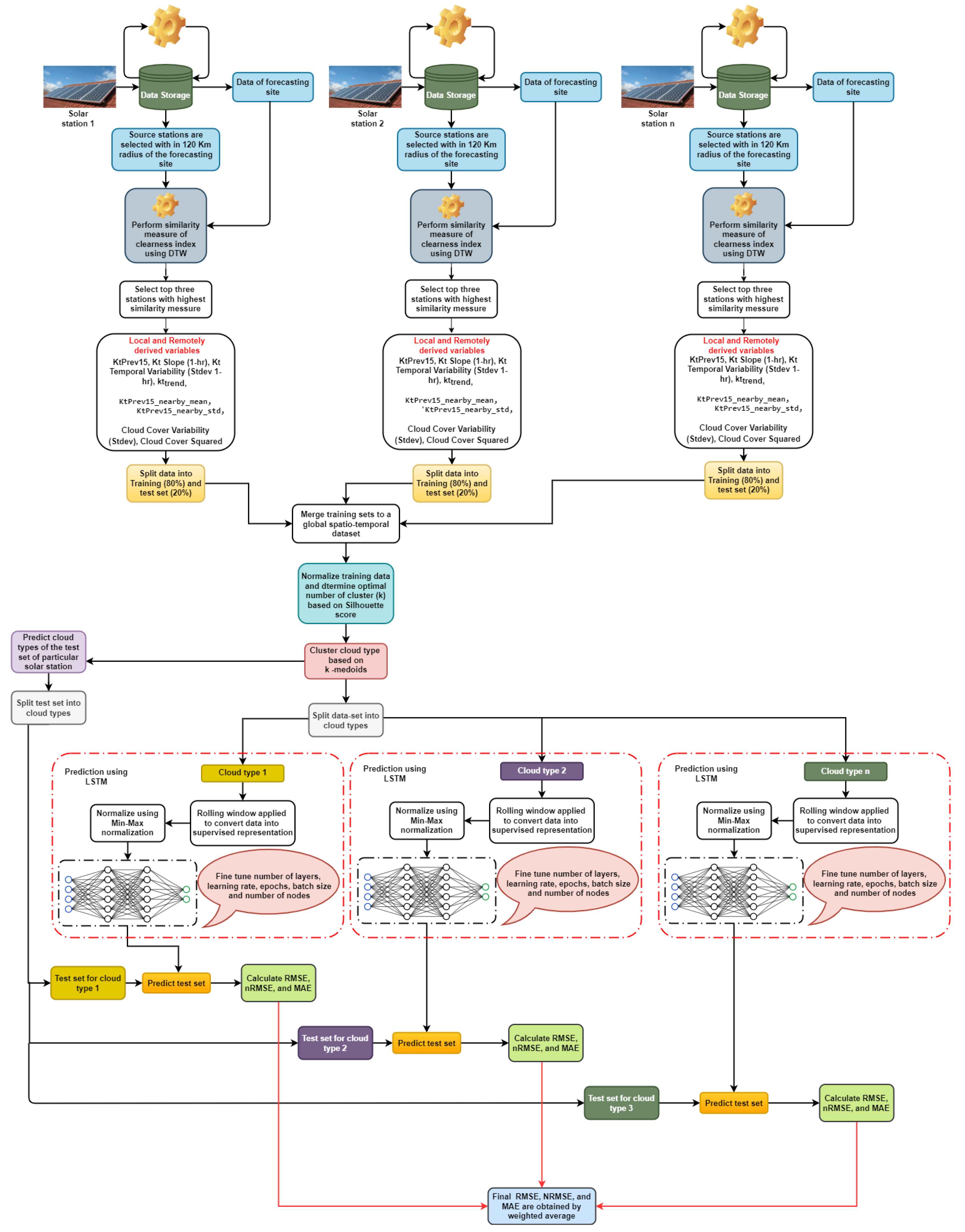
- For each forecasting site, the nearest three neighboring stations were selected on the basis of DTW similarity scores [26].
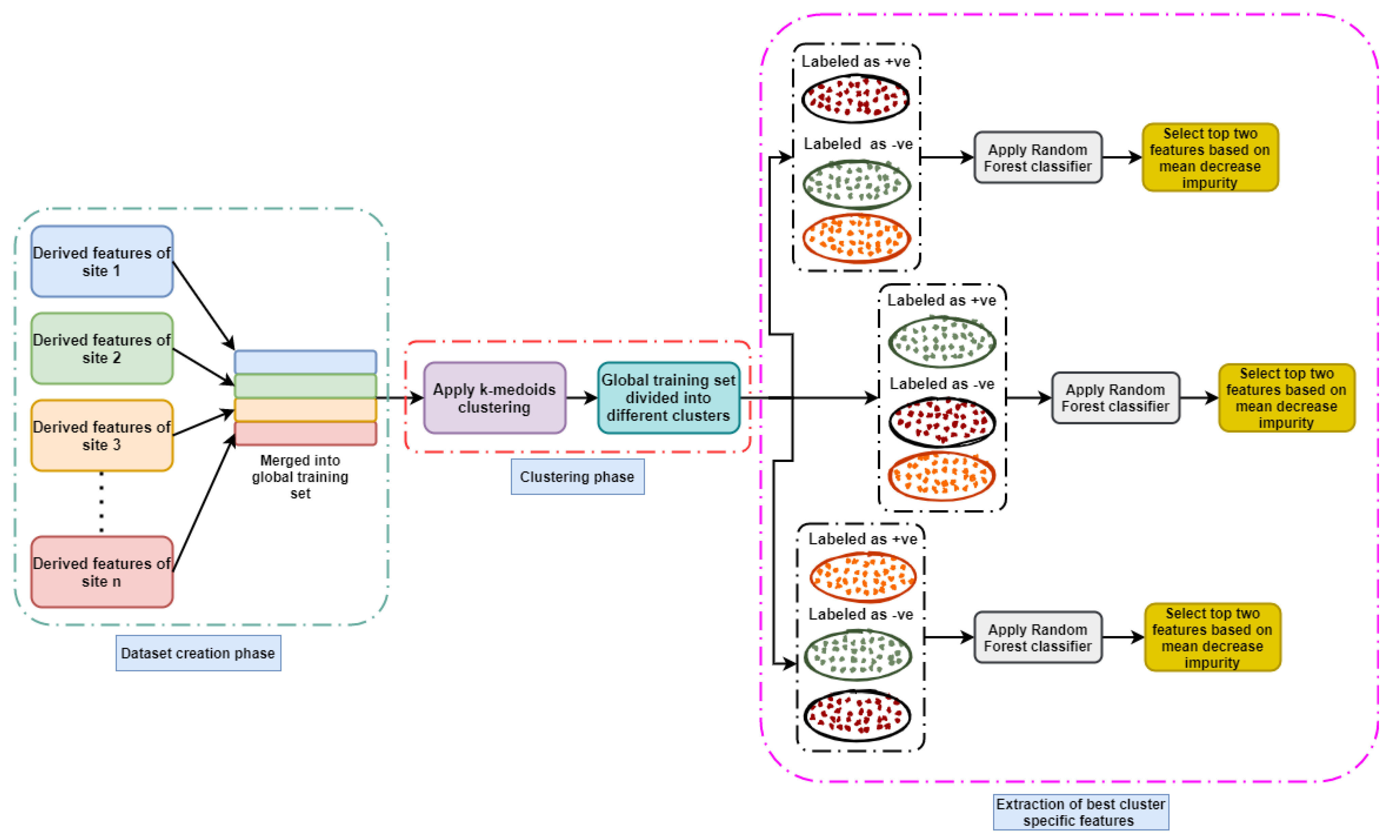
- A global dataset was created by combining some derived features of cloud cover and clearness indices of each station and those of its neighbors. The derived features were obtained following [23].
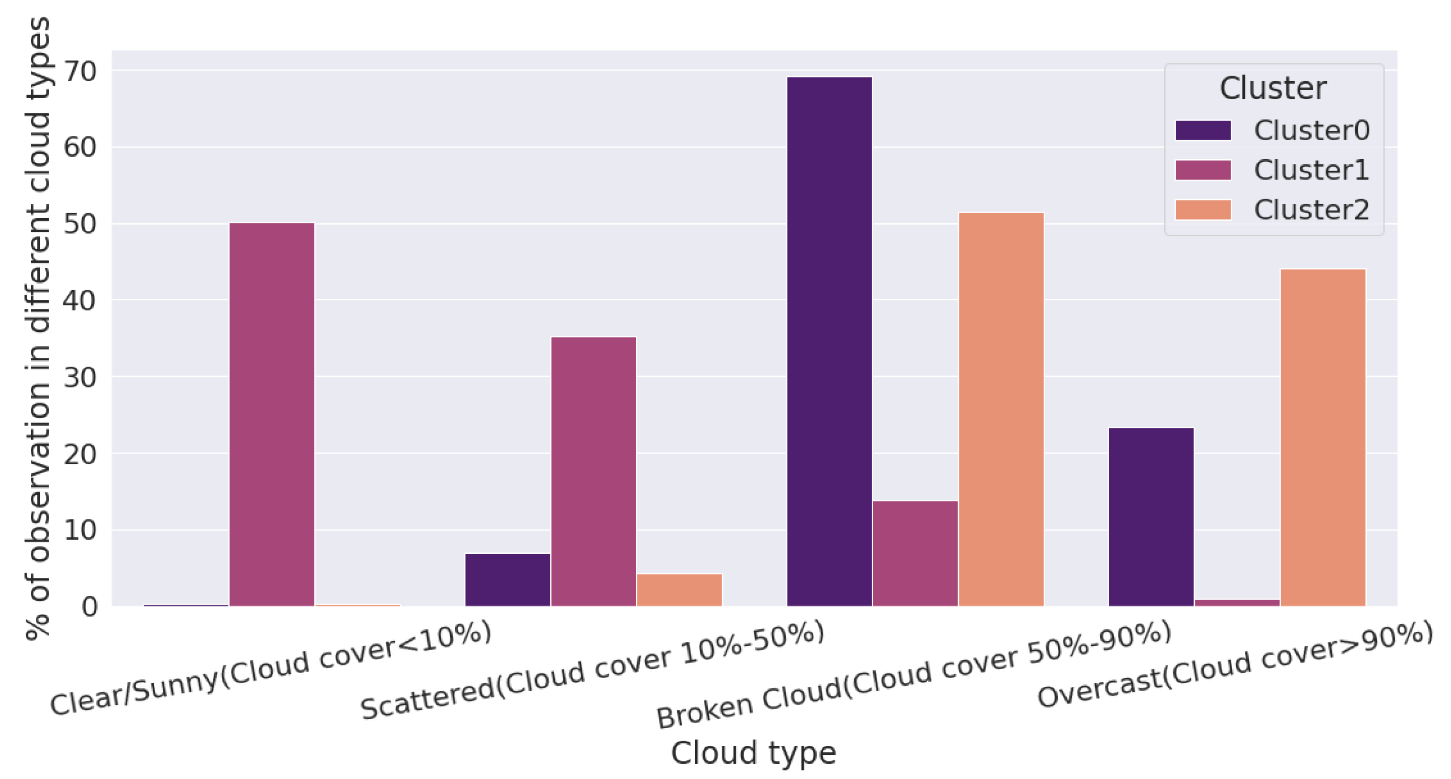
- The entire day was divided into time windows. For clustering, the K-medoids [27] algorithm was applied on those time windows.
- A separate LSTM model was trained for each cluster that represented different cloud conditions.
- An adaptive forecasting model (CB-LSTM) is proposed that can apply multiple models for a site on the basis of existing weather conditions.
- A global dataset was created on the basis of derived cloud-related information that is used to cluster a day into different weather types.
- The proposed model showed promising forecasting performance compared to benchmark models such as convolutional neural network (CNN)-LSTM and nonclustering-based site-specific LSTMs. The model achieved less forecasting error for solar stations having significant solar variability.
- Performance (measured in terms of forecasting accuracy) was validated for nine solar stations from three climatic zones in India. To our knowledge, this is the first time that such an approach was applied to data from the Indian subcontinent.
2. Deep-Learning Models
- Forget gate [29] : On the basis of certain conditions such as , , and a sigmoid layer, a forget gate produces either 0 or 1. If 1, memory information is preserved; otherwise, it is discarded.
- Input gate [29] : helps in deciding which values from the input are used for the current memory state.
- Cell state [29] : new cell state is the summation of , and . decides the fraction of the old cell state that is discarded, and the amount of new information that is added is decided through .
- Output gate [29] : decides what to output on the basis of the current input and previous hidden state.
- Hidden state [29] : current hidden state is computed by multiplying the output gate by the current cell state using the tanh function.
3. Materials and Methods
3.1. Dataset Description and Preprocessing
- Night hours (8 p.m. to 7 a.m.) are removed.The resolution of the collected data was 15 min.
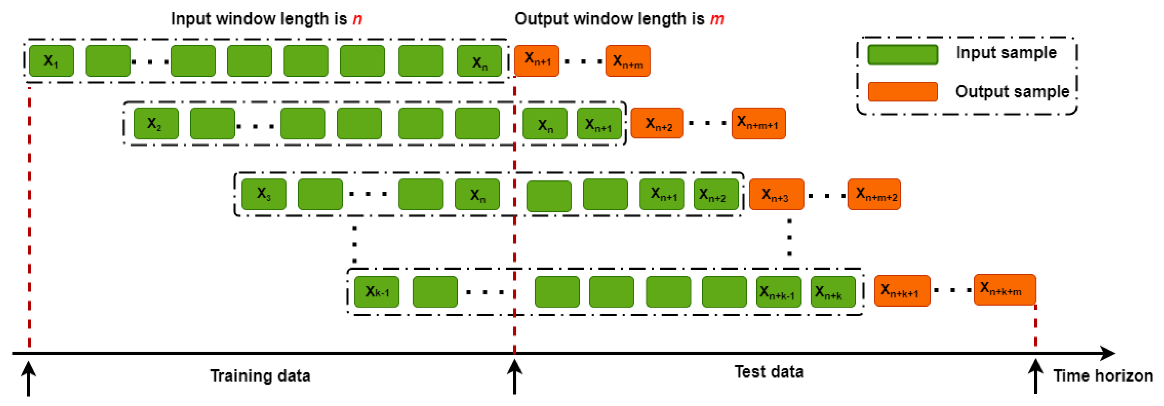
- Next, a standard sliding-window approach was applied to the time-series data to convert them into a suitable representation (supervised) for deep-learning models. Figure 4 depicts the generic approach of a sliding window with input and output window sizes n and m. The input window covered n past observations, such as {, , , …, }, and used to predict the next m observations as {, …, }. After that, the input window is shifted one position to the right as {, , , …, }, and {, …, } are the new input and output sequences. This process continues until no data points of the time series are left.
3.2. Locally and Remotely Derived Variables for Clustering
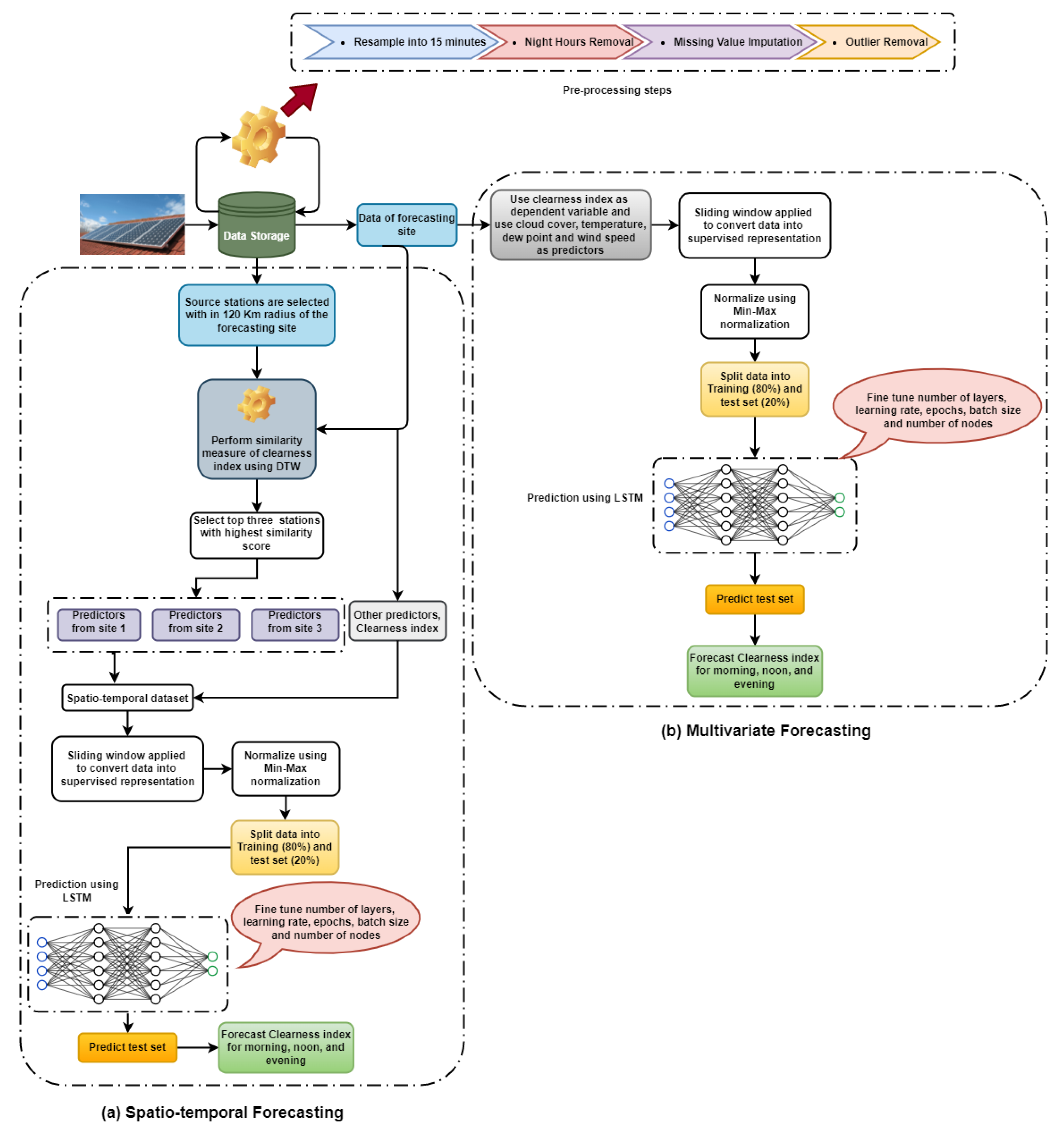
- A radius of 120 km was used to select the solar stations around the forecasting site.
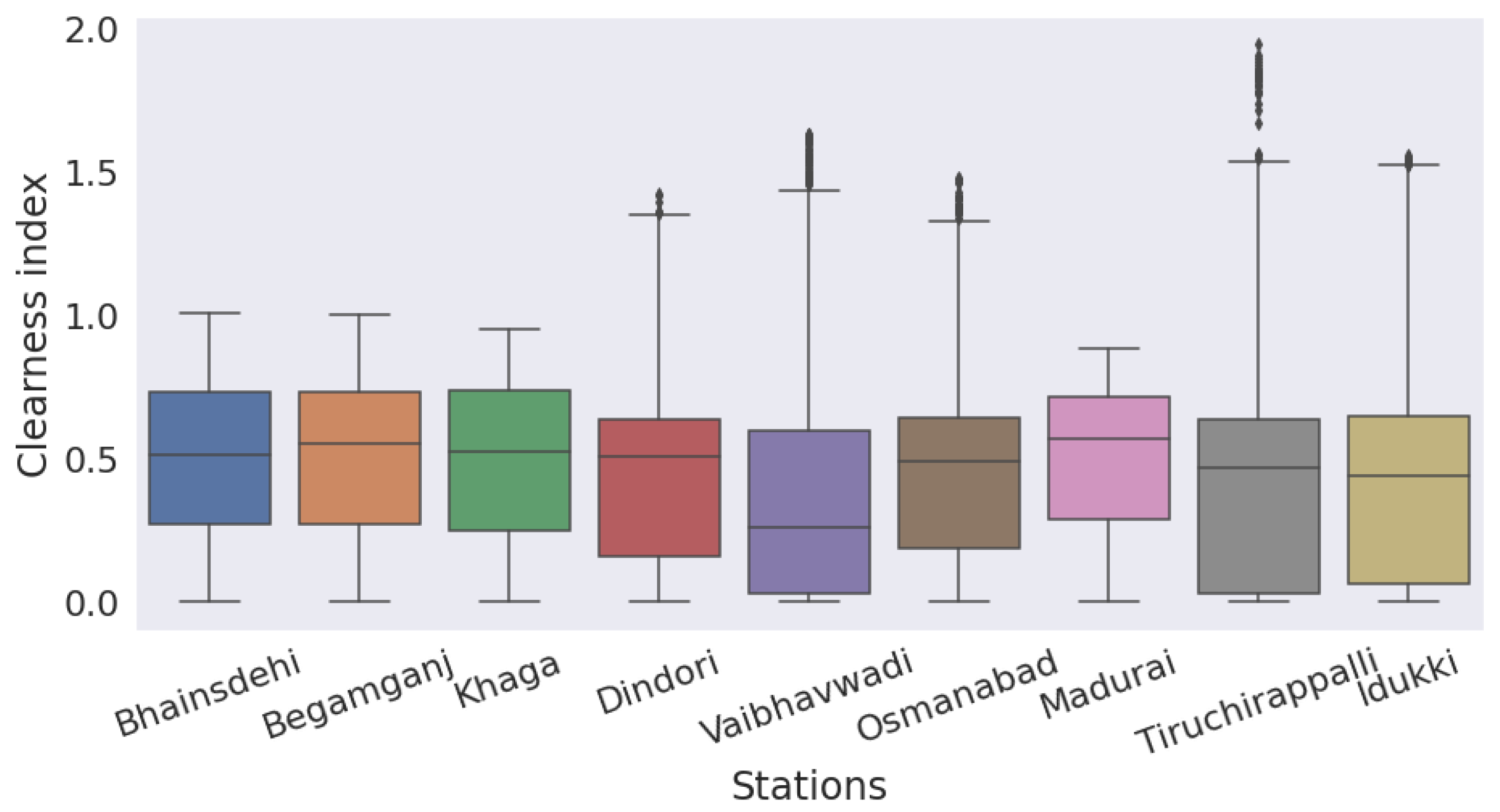
- DTW [32] was used as the similarity measure of clearness index (Kt).
- Three solar stations with the best similarity score were selected and used for clustering.
3.3. Multivariate LSTM (M-LSTM)
- It is a site-specific model where predictors are directly used from the forecasting site. The model uses additional information on predictors such as temperature, dew point, wind speed, and cloud cover.
- A stateful LSTM was used for maintaining inter- and intrabatch dependency. The input layer of an LSTM consists of 5 input features of 16 time steps (4 h) each. Two hidden layers and a tanh activation were used.
3.4. Spatiotemporal LSTM (ST-LSTM)
- A spatiotemporal dataset was created by combining information on meteorological parameters, including dew point, temperature, wind speed, and cloud cover from the three neighboring sites and from the forecast site.
- Stateful LSTM was used. The input layer consisted of 20 input features of 16 time steps each. Two hidden layers were used with a dropout rate of 20%. As hidden-layer activation, tanh was used.
- A spatiotemporal dataset was used to train the LSTM and forecast clearness index for three different times of the day.
3.5. Clustering-Based ANN (CB-ANN) and LSTM (CB-LSTM)
- For each cluster, separate stateless LSTM was built. The network was implemented using the keras package of version 2.7.0 in Python.The input layer of the LSTM consisted of 13 input features of 1 time step each. In the hidden layers, hyperbolic tangent activation function (tanh) was used. After each hidden layer, a batch-normalization [35] layer was used to transform inputs into a mean of 0 and a standard deviation of 1. We used a dropout and L2 regularization [36] to protect the network from overfitting. The network weights were initialized using the Xavier uniform initializer [37]. The output layer consisted of 8 nodes with linear activation and was used to forecast Kt for the next two hours. Figure 8 shows the network configuration of CB-LSTM together with input and output features. For obtaining the best performance of CB-LSTM, specific hyperparameters such as number of layers, number of nodes in each layer, batch size, number of epochs, dropout, and learning rate were optimized. The tree-structured Parzen estimator (TPE) [38] algorithm was used for optimization. Table 4 presents the hyperparameter settings. Table 5 shows the optimal hyperparameter settings for the proposed approach (CB-LSTM) in Section 4.
- Overall forecasting accuracy was computed for each site using the weighted average of the generated accuracy by the different LSTM models. Forecasting accuracy was separately computed for three times of the day.
3.6. Evaluation
4. Result and Discussion
5. Conclusions
Author Contributions
Funding
Institutional Review Board Statement
Informed Consent Statement
Data Availability Statement
Acknowledgments
Conflicts of Interest
References
- Elizabeth Michael, N.; Mishra, M.; Hasan, S.; Al-Durra, A. Short-Term Solar Power Predicting Model Based on Multi-Step CNN Stacked LSTM Technique. Energies 2022, 15, 2150. [Google Scholar] [CrossRef]
- Dudley, B. BP statistical review of world energy. In BP Statistical Review; BP p.l.c.: London, UK, 2018; Volume 6, p. 00116. [Google Scholar]
- Safi, M. India plans nearly 60% of electricity capacity from non-fossil fuels by 2027. The Guardian, 21 December 2016; 22. [Google Scholar]
- Gensler, A.; Henze, J.; Sick, B.; Raabe, N. Deep Learning for solar power forecasting—An approach using AutoEncoder and LSTM Neural Networks. In Proceedings of the 2016 IEEE International Conference on Systems, Man, and Cybernetics (SMC), Budapest, Hungary, 9–12 October 2016; pp. 002858–002865. [Google Scholar]
- Akarslan, E.; Hocaoglu, F.O. A novel adaptive approach for hourly solar radiation forecasting. Renew. Energy 2016, 87, 628–633. [Google Scholar] [CrossRef]
- Kumar, R.; Umanand, L. Estimation of global radiation using clearness index model for sizing photovoltaic system. Renew. Energy 2005, 30, 2221–2233. [Google Scholar] [CrossRef]
- Liu, B.; Jordan, R. Daily insolation on surfaces tilted towards equator. ASHRAE J. 1961, 10, 5047843. [Google Scholar]
- Perez, R.; Ineichen, P.; Seals, R.; Zelenka, A. Making full use of the clearness index for parameterizing hourly insolation conditions. Sol. Energy 1990, 45, 111–114. [Google Scholar] [CrossRef] [Green Version]
- Rajagukguk, R.A.; Ramadhan, R.A.; Lee, H.J. A Review on Deep Learning Models for Forecasting Time Series Data of Solar Irradiance and Photovoltaic Power. Energies 2020, 13, 6623. [Google Scholar] [CrossRef]
- Inman, R.H.; Pedro, H.T.; Coimbra, C.F. Solar forecasting methods for renewable energy integration. Prog. Energy Combust. Sci. 2013, 39, 535–576. [Google Scholar] [CrossRef]
- Yang, D.; Jirutitijaroen, P.; Walsh, W.M. Hourly solar irradiance time series forecasting using cloud cover index. Sol. Energy 2012, 86, 3531–3543. [Google Scholar] [CrossRef]
- Sanjari, M.J.; Gooi, H. Probabilistic forecast of PV power generation based on higher order Markov chain. IEEE Trans. Power Syst. 2016, 32, 2942–2952. [Google Scholar] [CrossRef]
- Feng, C.; Cui, M.; Hodge, B.M.; Lu, S.; Hamann, H.F.; Zhang, J. Unsupervised clustering-based short-term solar forecasting. IEEE Trans. Sustain. Energy 2018, 10, 2174–2185. [Google Scholar] [CrossRef]
- Bandara, K.; Bergmeir, C.; Smyl, S. Forecasting across time series databases using recurrent neural networks on groups of similar series: A clustering approach. Expert Syst. Appl. 2020, 140, 112896. [Google Scholar] [CrossRef] [Green Version]
- Hochreiter, S.; Schmidhuber, J. Long short-term memory. Neural Comput. 1997, 9, 1735–1780. [Google Scholar] [CrossRef] [PubMed]
- Wang, H.; Li, M.; Yue, X. IncLSTM: Incremental Ensemble LSTM Model towards Time Series Data. Comput. Electr. Eng. 2021, 92, 107156. [Google Scholar] [CrossRef]
- Abdel-Nasser, M.; Mahmoud, K. Accurate photovoltaic power forecasting models using deep LSTM-RNN. Neural Comput. Appl. 2019, 31, 2727–2740. [Google Scholar] [CrossRef]
- Aslam, M.; Lee, J.M.; Kim, H.S.; Lee, S.J.; Hong, S. Deep learning models for long-term solar radiation forecasting considering microgrid installation: A comparative study. Energies 2020, 13, 147. [Google Scholar] [CrossRef] [Green Version]
- Akhter, M.N.; Mekhilef, S.; Mokhlis, H.; Almohaimeed, Z.M.; Muhammad, M.A.; Khairuddin, A.S.M.; Akram, R.; Hussain, M.M. An Hour-Ahead PV Power Forecasting Method Based on an RNN-LSTM Model for Three Different PV Plants. Energies 2022, 15, 2243. [Google Scholar] [CrossRef]
- Qing, X.; Niu, Y. Hourly day-ahead solar irradiance prediction using weather forecasts by LSTM. Energy 2018, 148, 461–468. [Google Scholar] [CrossRef]
- Ali-Ou-Salah, H.; Oukarfi, B.; Bahani, K.; Moujabbir, M. A New Hybrid Model for Hourly Solar Radiation Forecasting Using Daily Classification Technique and Machine Learning Algorithms. Math. Probl. Eng. 2021, 2021, 6692626. [Google Scholar] [CrossRef]
- Yagli, G.M.; Yang, D.; Srinivasan, D. Automatic hourly solar forecasting using machine learning models. Renew. Sustain. Energy Rev. 2019, 105, 487–498. [Google Scholar] [CrossRef]
- McCandless, T.; Haupt, S.; Young, G. A regime-dependent artificial neural network technique for short-range solar irradiance forecasting. Renew. Energy 2016, 89, 351–359. [Google Scholar] [CrossRef] [Green Version]
- Yu, Y.; Cao, J.; Zhu, J. An LSTM short-term solar irradiance forecasting under complicated weather conditions. IEEE Access 2019, 7, 145651–145666. [Google Scholar] [CrossRef]
- Voyant, C.; Notton, G.; Kalogirou, S.; Nivet, M.L.; Paoli, C.; Motte, F.; Fouilloy, A. Machine learning methods for solar radiation forecasting: A review. Renew. Energy 2017, 105, 569–582. [Google Scholar] [CrossRef]
- Berndt, D.J.; Clifford, J. Using dynamic time warping to find patterns in time series. In Proceedings of the KDD Workshop, Seattle, WA, USA, 31 July 1994; Volume 10, pp. 359–370. [Google Scholar]
- Park, H.S.; Jun, C.H. A simple and fast algorithm for K-medoids clustering. Expert Syst. Appl. 2009, 36, 3336–3341. [Google Scholar] [CrossRef]
- Sharma, N.; Mangla, M.; Yadav, S.; Goyal, N.; Singh, A.; Verma, S.; Saber, T. A sequential ensemble model for photovoltaic power forecasting. Comput. Electr. Eng. 2021, 96, 107484. [Google Scholar] [CrossRef]
- Greff, K.; Srivastava, R.K.; Koutník, J.; Steunebrink, B.R.; Schmidhuber, J. LSTM: A search space odyssey. IEEE Trans. Neural Netw. Learn. Syst. 2016, 28, 2222–2232. [Google Scholar] [CrossRef] [Green Version]
- Gelaro, R.; McCarty, W.; Suárez, M.J.; Todling, R.; Molod, A.; Takacs, L.; Randles, C.A.; Darmenov, A.; Bosilovich, M.G.; Reichle, R.; et al. The modern-era retrospective analysis for research and applications, version 2 (MERRA-2). J. Clim. 2017, 30, 5419–5454. [Google Scholar] [CrossRef]
- Marion, B.; Kroposki, B.; Emery, K.; Del Cueto, J.; Myers, D.; Osterwald, C. Validation of a Photovoltaic Module Energy Ratings Procedure at NREL; Technical Report; National Renewable Energy Lab.: Golden, CO, USA, 1999. [Google Scholar] [CrossRef] [Green Version]
- Müller, M. Dynamic time warping. In Information Retrieval for Music and Motion; Springer: Berlin/Heidelberg, Germany, 2007; pp. 69–84. [Google Scholar] [CrossRef]
- Patro, S.; Sahu, K.K. Normalization: A preprocessing stage. arXiv 2015, arXiv:1503.0646. [Google Scholar] [CrossRef]
- Krishna, T.S.; Babu, A.Y.; Kumar, R.K. Determination of optimal clusters for a Non-hierarchical clustering paradigm K-Means algorithm. In Proceedings of International Conference on Computational Intelligence and Data Engineering; Springer: Berlin/Heidelberg, Germany, 2018; pp. 301–316. [Google Scholar] [CrossRef]
- Ioffe, S.; Szegedy, C. Batch normalization: Accelerating deep network training by reducing internal covariate shift. In Proceedings of the International Conference on Machine Learning, Lille, France, 7–9 July 2015; pp. 448–456. [Google Scholar]
- Cortes, C.; Mohri, M.; Rostamizadeh, A. L2 regularization for learning kernels. arXiv 2012, arXiv:1205.2653. [Google Scholar]
- Glorot, X.; Bengio, Y. Understanding the difficulty of training deep feedforward neural networks. In Proceedings of the Thirteenth International Conference on Artificial Intelligence and Statistics, Sardinia, Italy, 13–15 May 2010; pp. 249–256. [Google Scholar]
- Bergstra, J.; Bardenet, R.; Bengio, Y.; Kégl, B. Algorithms for hyper-parameter optimization. In Proceedings of the 25th Annual Conference on Neural Information Processing Systems (NIPS 2011), Granada, Spain, 12–17 December 2011; Volume 24. [Google Scholar]
- Shcherbakov, M.V.; Brebels, A.; Shcherbakova, N.L.; Tyukov, A.P.; Janovsky, T.A.; Kamaev, V.A. A survey of forecast error measures. World Appl. Sci. J. 2013, 24, 171–176. [Google Scholar] [CrossRef]
- Chai, T.; Draxler, R.R. Root mean square error (RMSE) or mean absolute error (MAE)?—Arguments against avoiding RMSE in the literature. Geosci. Model Dev. 2014, 7, 1247–1250. [Google Scholar] [CrossRef] [Green Version]
- Zang, H.; Liu, L.; Sun, L.; Cheng, L.; Wei, Z.; Sun, G. Short-term global horizontal irradiance forecasting based on a hybrid CNN-LSTM model with spatiotemporal correlations. Renew. Energy 2020, 160, 26–41. [Google Scholar] [CrossRef]


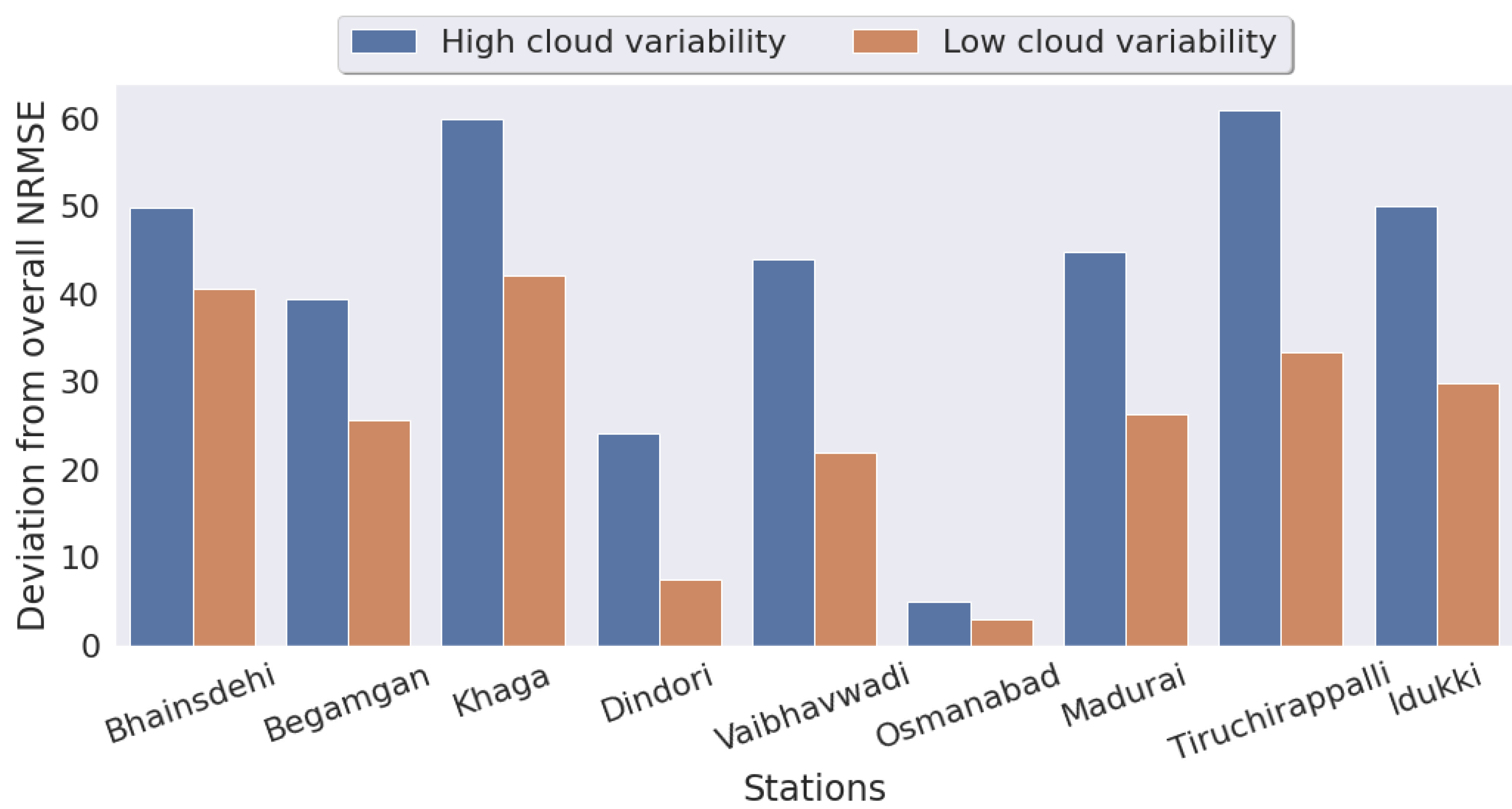
| Stations | High Cloud-Cover Variability | Low Cloud-Cover Variability | Overall NRMSE |
|---|---|---|---|
| Composite climate zone | |||
| Bhainsdehi | 44.72 | 17.71 | 29.85 |
| Begamganj | 39.03 | 20.80 | 27.98 |
| Dindori | 41.16 | 14.90 | 25.73 |
| Hot and dry climate zone | |||
| Tiruchirappalli | 59.06 | 44.02 | 47.57 |
| Idukki | 87.99 | 47.70 | 61.13 |
| Madurai | 47.89 | 44.29 | 45.65 |
| Warm and humid climate zone | |||
| Khaga | 34.23 | 17.42 | 23.63 |
| Vaibhavwadi | 92.22 | 38.22 | 57.31 |
| Osmanabad | 71.72 | 33.58 | 47.83 |
| Latitude and Longitude | Region | Climatic Zone | Location |
|---|---|---|---|
| 23.50 and 78.75 | Inland | Composite | Begamganj (Madhya Pradesh) |
| 22.50 and 81.25 | Inland | Composite | Dindori (Madhya Pradesh) |
| 25.50 and 81.25 | Inland | Composite | Khaga (Uttar Pradesh) |
| 21.50 and 77.50 | Inland | Hot and dry | Bhainsdehi (Madhya Pradesh) |
| 16.50 and 73.75 | Coastal | Hot and dry | Vaibhavwadi (Maharashtra) |
| 18.00 and 76.25 | Coastal | Hot and dry | Osmanabad (Maharashtra) |
| 10.00 and 78.125 | Inland | Warm and humid | Madurai (Tamil Nadu) |
| 11.00 and 78.75 | Coastal | Warm and humid | Tiruchirappalli (Tamil Nadu) |
| 10.00 and 76.875 | Coastal | Warm and humid | Idukki (Kerala) |
| Predictors | Equation | Description |
|---|---|---|
| Locally derived variables | ||
| It was calculated to capture the most recent trend | ||
| Kt temporal variability (Stdev 1-h) | Computed by taking the standard deviation of the four subsequent observations in an hour | |
| Kt Slope (1-h) | It was calculated by fitting a linear equation through four consecutive observations of the clearness index. | |
| Remotely derived variables | ||
| KtPrev15 nearby mean | ) | It was computed by taking the mean of the clearness index of three neighboring sites. |
| KtPrev15 nearby std | ) | It was computed by taking the standard deviation of the clearness index of three neighboring sites. |
| Cloud-cover variability (Stdev) | It is the standard deviation of the cloud cover of neighboring solar stations. | |
| Cloud Cover Squired | It is the squared value of the mean of cloud covers of three neighboring sites. | |
| Model | Hyperparameter | Value |
|---|---|---|
| Number of layers | 1, 2, 3 | |
| Nodes in layers | 25, 50, 75, 100 | |
| CB-LSTM | Learning rate | 0.1, 0.01, 0.001 |
| Batch size | 1, 10, 20, 50, 100 | |
| Epoch | 25, 50, 100, 150, 200 | |
| Dropout | 0.05, 0.1, 0.2 |
| Hyperparameters | Broken | Clear/Sunny | Broken/Overcast |
|---|---|---|---|
| Number of hidden layers | 2 | 2 | 2 |
| Nodes in hidden layer one | 100 | 25 | 100 |
| Nodes in hidden layer two | 100 | 25 | 100 |
| Learning rate | 0.001 | 0.001 | 0.001 |
| Batch size | 1 | 1 | 1 |
| Epochs | 200 | 200 | 100 |
| Dropout | 0.2 | 0.2 | 0.2 |
| Model parameters | 127,608 | 9408 | 127,608 |
| M-LSTM | ST-LSTM | |||||
|---|---|---|---|---|---|---|
| Forecasting Sites | RMSE | NRMSE | MAE | RMSE | NRMSE | MAE |
| Composite | ||||||
| Bhainsdehi | 0.1429 | 0.2550 | 0.0870 | 0.1408 | 0.2515 | 0.0812 |
| Begamganj | 0.2211 | 0.3568 | 0.0952 | 0.2090 | 0.3410 | 0.0960 |
| Dindori | 0.2430 | 0.3541 | 0.1258 | 0.2164 | 0.3352 | 0.1358 |
| Hot and dry | ||||||
| Tiruchirappalli | 0.2859 | 0.5426 | 0.1894 | 0.2854 | 0.5419 | 0.1888 |
| Idukki | 0.3087 | 0.6243 | 0.1957 | 0.2969 | 0.6037 | 0.1837 |
| Madurai | 0.2725 | 0.5497 | 0.1746 | 0.2704 | 0.5447 | 0.1845 |
| Warm and humid | ||||||
| Khaga | 0.2253 | 0.3888 | 0.1049 | 0.1890 | 0.3300 | 0.1113 |
| Vaibhavwadi | 0.2911 | 0.4708 | 0.1821 | 0.2726 | 0.4423 | 0.1831 |
| Osmanabad | 0.3001 | 0.4541 | 0.2188 | 0.2896 | 0.4408 | 0.1941 |
| CB-LSTM | CB-ANN | ST-LSTM | |||||||
|---|---|---|---|---|---|---|---|---|---|
| Forecasting Sites | RMSE | NRMSE | MAE | RMSE | NRMSE | MAE | RMSE | NRMSE | MAE |
| Composite | |||||||||
| Bhainsdehi | 0.1096 | 0.1936 | 0.0677 | 0.1569 | 0.2762 | 0.1243 | 0.1408 | 0.2515 | 0.0812 |
| Begamganj | 0.1148 | 0.2016 | 0.0751 | 0.1664 | 0.3118 | 0.1384 | 0.2090 | 0.3410 | 0.0960 |
| Dindori | 0.1426 | 0.2530 | 0.1079 | 0.1790 | 0.3440 | 0.1445 | 0.2164 | 0.3352 | 0.1358 |
| Hot and dry | |||||||||
| Tiruchirappalli | 0.1605 | 0.2903 | 0.1094 | 0.1617 | 0.3414 | 0.1173 | 0.2854 | 0.5419 | 0.1888 |
| Idukki | 0.2118 | 0.4934 | 0.1339 | 0.2001 | 0.5288 | 0.1376 | 0.2969 | 0.6037 | 0.1837 |
| Madurai | 0.1793 | 0.3208 | 0.1193 | 0.1619 | 0.3288 | 0.1447 | 0.2704 | 0.5447 | 0.1845 |
| Warm and humid | |||||||||
| Khaga | 0.1483 | 0.2641 | 0.1139 | 0.1623 | 0.3195 | 0.1258 | 0.1890 | 0.3300 | 0.1113 |
| Vaibhavwadi | 0.2009 | 0.3599 | 0.1200 | 0.2109 | 0.4980 | 0.1475 | 0.2726 | 0.4423 | 0.1831 |
| Osmanabad | 0.1879 | 0.3757 | 0.1089 | 0.2238 | 0.4760 | 0.1595 | 0.2896 | 0.4408 | 0.1941 |
| Forecasting Sites | CB-LSTM | [21] | [41] | [23] |
|---|---|---|---|---|
| Composite | ||||
| Bhainsdehi | 19.36% | 22.75% | 26.09% | 27.62% |
| Begamganj | 20.16% | 20.74% | 26.39% | 31.18% |
| Dindori | 25.30% | 25.09% | 27.93% | 34.40% |
| Hot and dry | ||||
| Tiruchirappalli | 29.03% | 38.06% | 47.62% | 34.14% |
| Idukki | 49.34% | 49.82% | 54.04% | 52.88% |
| Madurai | 32.08% | 34.14% | 47.67% | 32.88% |
| Warm and humid | ||||
| Khaga | 26.41% | 20.90% | 24.02% | 31.95% |
| Vaibhavwadi | 35.99% | 45.70% | 46.61% | 49.80% |
| Osmanabad | 37.57% | 48.89% | 41.98% | 47.60% |
Publisher’s Note: MDPI stays neutral with regard to jurisdictional claims in published maps and institutional affiliations. |
© 2022 by the authors. Licensee MDPI, Basel, Switzerland. This article is an open access article distributed under the terms and conditions of the Creative Commons Attribution (CC BY) license (https://creativecommons.org/licenses/by/4.0/).
Share and Cite
Malakar, S.; Goswami, S.; Ganguli, B.; Chakrabarti, A.; Roy, S.S.; Boopathi, K.; Rangaraj, A.G. Deep-Learning-Based Adaptive Model for Solar Forecasting Using Clustering. Energies 2022, 15, 3568. https://doi.org/10.3390/en15103568
Malakar S, Goswami S, Ganguli B, Chakrabarti A, Roy SS, Boopathi K, Rangaraj AG. Deep-Learning-Based Adaptive Model for Solar Forecasting Using Clustering. Energies. 2022; 15(10):3568. https://doi.org/10.3390/en15103568
Chicago/Turabian StyleMalakar, Sourav, Saptarsi Goswami, Bhaswati Ganguli, Amlan Chakrabarti, Sugata Sen Roy, K. Boopathi, and A. G. Rangaraj. 2022. "Deep-Learning-Based Adaptive Model for Solar Forecasting Using Clustering" Energies 15, no. 10: 3568. https://doi.org/10.3390/en15103568
APA StyleMalakar, S., Goswami, S., Ganguli, B., Chakrabarti, A., Roy, S. S., Boopathi, K., & Rangaraj, A. G. (2022). Deep-Learning-Based Adaptive Model for Solar Forecasting Using Clustering. Energies, 15(10), 3568. https://doi.org/10.3390/en15103568