Residential Fuel Transition and Fuel Interchangeability in Current Self-Aspirating Combustion Applications: Historical Development and Future Expectations

Abstract

To reduce greenhouse gases and air pollutants, new technologies are emerging to reduce fossil fuel usage and to adopt more renewable energy sources. As the major aspects of fuel consumption, power generation, transportation, and industrial applications have been given significant attention. The past few decades witnessed astonishing technological advancement in these energy sectors. In contrast, the residential sector has had relatively little attention despite its significant utilization of fuels for a much longer period. However, almost every energy transition in human history was initiated by the residential sector. For example, the transition from fuelwood to cheap coal in the 1700s first took place in residential houses due to urbanization and industrialization. The present review demonstrates the energy transitions in the residential sector during the past two centuries while portending an upcoming energy transition and future energy structure for the residential sector. The feasibility of the 100% electrification of residential buildings is discussed based on current residential appliance adoption, and the analysis indicates a hybrid residential energy structure is preferred over depending on a single energy source. Technical considerations and suggestions are given to help incorporate more renewable energy into the residential fuel supply system. Finally, it is observed that, compared to the numerous regulations on large energy-consumption aspects, standards for residential appliances are scarce. Therefore, it is concluded that establishing appropriate testing methods is a critical enabling step to facilitate the adoption of renewable fuels in future appliances.

1. Introduction

When fossil fuel consumption and its impact on climate change is discussed, power generation, transportation, and industrial applications receive significant attention due to their large market share and the advanced technologies being developed and adopted by these sectors. An aspect that generally receives little attention is the residential energy sector.

The urbanization and industrialization of England in the 1700s forced London residents to abandon the use of suddenly expensive fuelwood and turn to cheaper coal. Since then, the residential sector has always been in the pioneer position relative to energy transition in the world. The large use of fossil fuels during and after the Industrial Revolution emerged after residential markets had created a thriving trade [1,2].

The past few decades have witnessed astonishing combustion technology advancement in gas turbines, internal combustion engines, and other industrial applications. Moreover, the strict emission regulations on high-energy-consuming devices greatly boosted their combustion technology advancement. Take heavy-duty gas turbines, for example: water was injected into the combustor to reduce NO_X emissions in the 1970s. As emission regulations are becoming more stringent, numerous technologies have been developed to reduce NO_X emissions, including rich burn-quick mix-lean burn (RQL) technology [3], dry low NO_X (DLN) lean premixed combustion [4], mild combustion [5], etc. Post-combustion pollutant-elimination technologies, such as Selective Catalytic Reduction (SCR), are also being adopted to further decrease gas turbine NO_X emissions down to the single-digit ppm level [6]. Although the emission levels of the high-energy-consumption units are already very low, a lot of investment and effort is still being invested to further decrease or possibly eliminate the emissions from those devices altogether. In contrast, the emission level of some appliances can stay at around a couple hundred ppm without attracting much attention from policymakers. Moreover, the combustion technologies used in gas appliances are the same as 100 years ago, which were mainly adopted from Bunsen flames [7,8].

As more renewable energy technologies are being developed, the idea of incorporating solar panels, wind turbines, batteries, fuel cell units, etc., into residential homes is also promising [9,10]. Discussions have occurred regarding the 100% electrification of residential homes to eliminate both the greenhouse gas emissions and air pollution from the residential sector and shift them to power-generation units, which might make pollutantssrelatively easy to be regulated and controlled [11,12]. However, very few studies considered the current status of gas and electric appliances’ market share and the potential for an increase in carbon emissions due to the 100% electrification of residential appliances.

Renewable gases such as biogas and renewable hydrogen are becoming available at a much lower price than most non-combustion renewable energy sources and can also be generated from multiple renewable sources. For example, biogas can be produced from wood and agricultural products, landfill waste, sewage, etc. [13]. Injecting purified biogas into existing natural gas pipelines has already been adopted and has gained much success in reducing carbon emissions [14]. Besides biogas, hydrogen is also a competitive and promising fuel for the future due to its high energy density on the mass base and the many ways it can be generated. The carbon-free property of hydrogen inherently reduces greenhouse gas emissions when generated renewably. Renewable sources for hydrogen include biomass, solar energy, wind power, and water electrolysis using grid power [15,16]. The adoption of these renewable gases in existing natural gas pipelines should be easier and cheaper for end users without much capital investment and maintenance. Biogas or hydrogen injection into the existing natural gas pipeline needs technical evaluation and fuel-interchangeability studies. However, gas appliance manufacturers and gas utility companies are still using the flame indices from the 1920s to guide their fuel-interchangeability investigations. Therefore, more comprehensive considerations should be given to guide appliance performance upgrades while adopting renewable fuels.

As many future fuel choices and energy-consumption structures are being predicted, this paper summarizes the historical energy transitions in the residential sector and their interactions with other sectors. The past experience allows us to glimpse the future energy structure. The feasibility of electrifying residential homes by 100% is discussed based on the comparison between the existing electric/gas appliances and their energy consumption. Furthermore, the technical considerations of fuel interchangeability in residential appliances are summarized and discussed, including combustion technologies, fuel properties, and flame indices. The lack of international standard testing methods and regulations on residential appliances and the representative regional regulations on appliance performance are also summarized.

2. Residential Fuel Consumption Historical Variation

The fuel consumption shares among different energy sources vary along with human society’s development. Figure 1 shows the energy consumption variation for the past two centuries of the U.S.. Before the 19th century, wood was the dominant fuel. With the start of the Industrial Revolution, wood could no longer meet the massive energy demand due to its low energy density and the supply scarcity caused by fast forest destruction. Meanwhile, coal consumption significantly increased with its worldwide discovery and the advancement of coal-mining technologies. Coal consumption surpassed that of wood in the late 19th century and played an essential role in the Industrial Revolution. The oil and gas industry started to rise around the 1900s, and their market share surpassed coal consumption in the 1950s. Till today, oil, natural gas, and coal still dominate the energy sources in the world.

The energy transitions of the U.K., France, Netherland, Russia, Japan, China, Nigeria, etc., were also investigated [18,19,20]. Although the timeline or specific numbers differ, a similar trend of energy transition was found worldwide: from biomass (crop residuals, fuelwood, etc.) to coal, then oil and gas, and afterward from fossil fuel to nuclear or other renewable powers.

Although power generation, transportation, and industrial applications reflect the majority of fuel consumption, the residential sector is also an important and often the most price-sensitive sector relative to fuel utilization. Yet, this sector has significantly fewer technological advancements and research development, likely due to the low profit margins and relatively low cost associated with appliances. However, it was noted that domestic energy consumption and needs shaped the use of energy sources, especially at the initial stage of their rise [21,22,23,24,25,26,27]. Therefore, investigating the residential section of energy consumption is of great importance, especially in considering future fuel consumption scenarios. The following sections summarize the development of residential fuel consumption.

2.1. Before the 1900s: Transition from Wood to Coal

The transition from wood to coal in the residential sector was accompanied by population growth and the rapid development of industry. This combined effect created a large increase in demand for fuelwood. As fuelwood became more limited, people sought alternative fuels to replace what potentially looked like increasingly more expensive fuelwood. This residential fuel transition, on a massive scale, first occurred in England.

The population in England increased dramatically by more than 80%, from 3.02 million in 1541 to 5.47 million in 1656 [28]. Despite this, the population explosion did not exert a significant influence on the fuelwood supply for residential houses. Residential fuelwood could still be secured in a lot of regions by planting trees in backyards, on roadsides, on otherwise infertile slope land, or in fuelwood groves to supply nearby farms or villages [18]. In England, the fuelwood prices were actually fairly stable between 1550 and 1650 [29]. Wilson [30] also noted that, from 1450 to 1650, while timber prices in England increased, they did not increase as much as the cost of other agricultural products. In fact, timber became cheaper year by year relative to inflation, even with increasing demand from the residential sector. Hence, the population growth did not exert a high demand for wood supply and was not the major reason for the fuelwood price increase. It was the rise of industry that exhausted the fuelwood supply and drove up the price significantly. It forced the residential sector to seek alternative fuels other than fuelwood.

Before the 18th century, industry applications also used fuelwood as their energy source. Surprisingly, even though coal possesses more than 33% more energy density than fuelwood and at a lower price, the industry did not switch their fuel from fuelwood to coal very quickly. The smoky and sulfurous nature of coal made its adoption difficult for industries that required smokeless or odorless fuels [31]. Further, the slow transition from fuelwood to coal in industry was not because of a lack of clean coal-burning technology, but more because the industry was still profiting a lot from burning fuelwood. The energy density benefit of replacing fuelwood with coal could not balance out the capital investment of adjusting the combustion devices and coal transportation. Similar to the current situation, momentum in the industry and conservative tendencies usually slow new technology adoption. Fuel interchangeability studies from fuelwood to coal in industrial applications were already conducted in the Elizabethan Age. In 1590, John Thornbrough, the Dean of York, was granted a seven-year project to remove the “piercing and acrimonious spirits” for beer making and processing alum. By 1610, there were already patent applications using coal as fuel in the baking of malt, bread, bricks, tiles, and smelting of bell metal copper, brass, iron, lead, and glass [32,33]. Although the possibility of utilizing coal was realized and numerous studies were conducted to adapt combustion devices from wood to coal, coal remained an insignificant industry fuel until the 17th century.

With the development of industrial technologies, fuelwood could not meet the energy demand anymore due to its low energy density and limited supply caused by the slow recovery of forests. According to the study results on historical energy consumption, 20 kg of charcoal could only produce 1 kg of iron (600 MJ/kg) in England during the Middle Ages [18]. The glass industry was also wood-intensive. To produce 1 kg of glass, 2.4 tons of wood needed to be consumed for both heating and to obtain potassium (90 MJ/kg). Salt production is also a major wood-consuming sector, which demands as much as 500–600 MJ wood consumption per kilogram of salt produced [34]. This large amount of fuelwood requirement in the industrial sector caused severe forest destruction, and eventually, fuelwood prices increased. Therefore, residents sought cheaper alternative fuels. In the latter half of the 17th century, the coal price in England was less than half of fuelwood per unit of gross energy [35]. This fuel price gap between fuelwood and coal was more significant in densely populated London than the England average. In

Table 1. Indices of estimated price movements in London, 1451–1642.

Commodity	1451–1500	1531–1540	1551–1560	1583–1592	1603–1612	1613–1622	1623–1632	1633–1642
General	100	105	132	198	251	257	282	291
Fuelwood	100	94	163	277	366	457	677	780
Coal	100	89	147	186	295	371	442	321

[19], the fuel prices and the general living cost level in London are normalized to 100 from the year 1451 to 1500. It can be seen that coal saw a steady increasing trend with the living cost over the next 190 years. Fuelwood prices started to increase significantly by the end of the 1500s. By 1642, the cost of fuelwood was more than double the price of coal.

As the residents in London increasingly adopted coal as the substitute for fuelwood, imports of coal to London increased significantly in the last decade of the 16th century.

Table 2. Imports of coal into London, 1580s–1680s.

Year	Period	Tons	Notes
1580	12 March–18 September	10,785
1585–1586	Michaelmas–Michaelmas	23,867
1591–1592	Michaelmas–Michaelmas	34,757
1605–1606	Christmas–Christmas	73,984
1614–1615		91,599	One week missing
1637–1638		142,579	Two weeks missing; a year of bad trade
1667–1668	Midsummer–Midsummer	264,212
1680–1681	Michaelmas–Michaelmas	361,189

[36] shows the coal imports records from the late 16th century to the late 17th century. As can be seen, the coal consumption in London increased significantly from 10,785 tons to 361,189 tons in a century.

It should be noted that this coal consumption increase was mainly caused by the residential sector’s needs, since the technology for using coal in industry was still not widely adopted in the 17th century. The evidence for this can be found in the iron industry. In the 17th century, iron smelting was a voracious consumer of fuelwood in London. The dependence of smelting on the increasingly scarce and high-priced fuelwood supplies in the 17th century led to a situation in which the conversion of iron ore into metal in England was temporarily checked. However, this situation did not make the iron industry turn to coal combustion. Instead, a policy was released by the government to encourage imports of intermediate product pig iron instead of raw iron ore. Therefore, the rapid growth of coal production from the mid-16th century to the late 17th century largely represents the substitution of coal for wood as a household fuel [19].

The earliest coal shipped to London was from Newcastle as ballast, which was known as “sea-coal” [37]. The burning of sea-coal was reported to cause smoke with a pungent odor [38]. Therefore, presumably, sea-coal was of low quality and might have had a relatively high sulfur content. Sea-coal was first adopted by the poor residents in London due to its cheap price. To adapt the wood-burning fireplace to sea-coal, chimneys were built or modified to vent the smoke out of the house. Therefore, the number of chimneys of residential houses in London increased greatly around the 1550s. The acceptance of sea-coal by the upper classes and nobility followed the steps of lower-class residents with a time lag. The use of sea-coal as a domestic heating source in royal house was a slow process since Queen Elizabeth I was “greatly grieved and annoyed with the taste and smoke of sea-coal”. After her death in 1603, James VI of Scotland became James I of England, during whose governing period the popularity of using coal in residential houses was gained. Scotland was short of wood but had less indigenous sulfurous coal, which led to coal being used in houses of Scottish nobles much earlier than in England. Therefore, the new king continued his old habit of using coal for domestic heating in England. Such behavior aided the adoption of coal as a domestic fuel for wealthy London households [32].

It was the high demand for coal consumption in residential households that spurred the early development of coal mining and transportation. Coal provided the power source for and encouraged the Industrial Revolution. Although a bit later, the U.S. went along a very similar pathway in the fuel transition from fuelwood to coal. In the U.S., coal surpassed fuelwood’s energy supply in the 19th century, which was around 200 years later than the energy transition of Britain [39]. The early records in the U.S. of coal trading were in Pennsylvania, and the major market for the first decade of the anthracite coal trade in Pennsylvania was in American homes [24,40]. Therefore, when the early coal boosters tried to quantify the potential market in New York, they counted the numbers of homes, not the numbers of factories or steam engines [21].

Similar to the situation of Britain, the early coal utilization in the U.S. was hindered by the poor transportation situation around the coalfields on the East Coast. Even if Pennsylvania’s anthracite coalfields were only a hundred miles away from the eastern seaboard, transporting coal to Philadelphia and New York was still extremely expensive in the early 19th century. In the year 1810, it cost more to ship coal fewer than a hundred miles to Philadelphia than it did to deliver comparable shipments three thousand miles from England [41]. However, the War of 1812 tripled the price of imported coal from Britain. During this time, emphasis on energy security resulted in local anthracite coal in Philadelphia gaining a higher market share on the East Coast [42]. The real booster of the U.S. domestic coal consumption on the East Coast was the construction of the Schuylkill Canal in the 1820s. The Canal decreased coal’s transportation cost significantly. In the 1810s, one ton of anthracite coal cost around 20 U.S. dollars. However, this price kept dropping to 8.4 dollars in 1820 and then 6.5 dollars in 1830. In the 1840s, the coal price on the East Coast of the U.S. decreased to around 4 dollars per ton [43]. Due to the availability of cheap coal, fuel-interchangeability studies on fuelwood to coal in residential appliances were conducted by scientists and appliance manufacturers. Between the years 1815 and 1839, 329 patents for coal-combustion stoves were issued in the U.S. [44]. In the early adoption stage, a coal-burning stove cost around 30 dollars, while the average laborer only earned 2 dollars a day [45]. However, by the early 1830s, a domestic coal stove cost less than 10 dollars [21].

The Industrial Revolution further sped up the energy transition from fuelwood to coal, especially when steam engines became widely adopted in the late 18th and early 19th centuries. However, as noted above, this energy transition was first initiated by the residential sector. After coal was widely adopted in residential cooking and heating, the accessibility of cheap coal paved its way to more applications in industry, thus fostering the Industrial Revolution.

2.2. From the 19th Century to the 1950s: Coal to Manufactured Gases

Besides the transition to coal utilization, the residential market also played an essential role in the development of the petroleum industry and trade, especially in its initial development stage in the latter half of the 19th century. The combination of urbanization and industrialization in both America and Europe led to a great need for lighting. Therefore, petroleum was first refined to obtain kerosene, which was a lighting source to replace diminishing and increasingly expensive whale oil [21,27,46,47]. The early development era of the petroleum industry is also called “The Age of Illumination” [48].

At the early age of the oil industry, instead of being a major petroleum product as it is today, gasoline was only a surplus byproduct that was usually burned at refineries, converted to gaseous fuel for gas lights, or just dumped into the atmosphere due to its high volatility. Being a waste product, cheap gasoline stimulated the development of engines in the late 19th and early 20th centuries. For example, when Mercedes entered the U.S. market in the early 20th century, the price per car was USD 12,450 (~USD 374 k in 2021 values), but the gasoline price was only 7 cents/gallon (around USD 2/gallon in 2021 values) [47]. With the accessibility of cheap and abundant gasoline, the auto industry invested more money into automobile technologies, and the prices dropped significantly. For example, when Ford first introduced its Model T to the market in 1908, the price was USD 950, which dropped down to USD 269 by 1923 [49]. Before electric lighting and automobiles gained popularity in the first decade of the 20th century, kerosene was the major focus of the petroleum industry for providing light. Since the beginning of the petroleum industry, techniques were focused on maximizing the production of kerosene until the second decade of the 20th century. As shown in Figure 2, although most crude oil is refined to gasoline and diesel today, in the 1870s, more than 80% of a barrel of crude petroleum was transformed into illuminating oil [17,48].

As petroleum (kerosene) found its use in domestic lighting applications in the late 19th century and early 20th century, the energy transition in domestic cooking and heating changed from coal to different kinds of manufactured gases. Although it is hard to track who was the first to produce manufactured gas, Becker and Clayton are believed to be the early pioneers who invented methods to produce combustible gases from coal. In 1681, Johann Becker from Germany discovered that combustible gases could be generated by heating coal in the absence of air. Three years later, John Clayton from England collected combustible gas using a similar coal treatment method and called this gas the “Spirit of Coals”. The commercialization of manufactured gas in residential and industrial applications was initiated by the foundation of London and Westminster Gas Light and Coke Company in 1812. In the same year, this company built the world’s first commercialized gas networks in Great Peter Street, Westminster, London, by laying wooden pipes and illuminated Westminster Bridge with gas lamps on New Year’s Eve in 1813 [50]. Due to its clean combustion performance and ease of transporting through pipelines compared to coal, manufactured gas quickly gained popularity in the early 19th century. The prosperity of the gas industry was accompanied by emerging inventions of gas-combustion appliances. In 1826, the world’s first gas stove was designed in England by James Sharp [51]. In the 1850s, Robert Bunsen invented the aspirated burner (Bunsen burner), which significantly influenced gas applications in residential and industrial applications till today [52]. In the 1870s, Dr. Carl Auer von Welsbach invented the incandescent gas light mantle, which solved the inefficient combustion of open-flame burners in streetlamps [53]. Moreover, water heaters, room heaters, and many other appliances, such as soldering irons and hair-curling tongs, appeared on the scene in the mid- to late 1800s [50]. To meet the increasing customer base, more gas networks were built in Britain along with manufactured gas production sites, which are shown in Figure 3. Due to the widespread application of manufactured gas in the cities of Britain, manufactured gas was also called “town gas” in the U.K. [54].

The United States started the manufactured gas era at the same time as Britain. In 1816, the first manufactured gas company in America—the Gas Light Company of Baltimore—was founded. On 7 February 1817, the first manufactured gas streetlamp was lit in Baltimore. This was followed by the foundation of the Boston Gas Light Company in 1822 and the New York Gas Light Company in 1825 [50].

It should be noted that the early manufactured gas companies generated their gases from coal, except for the Gas Light Company of Baltimore, which produced its gases from the distillation of pine tar. However, the company switched to coal gas in 1822 due to the maturity of the coal gas production technologies and more satisfactory gas qualities [50]. Manufactured gas is a general term for multiple man-made gases, including coal gas, producer gas, water gas, carbureted water gas, oil (petroleum) gas, etc. The name of a particular manufactured gas depends on both the source and the gas production procedure. Overlaps in the naming system for manufactured gases are apparent. For example, producer gas can also be called coal gas if it is generated by coal. Water gas is produced in a gasification process in a carbon fuel bed with steam, and coal is decomposed into hydrogen and carbon monoxide [56]. Carbureted water gas is water gas with added carbon contents to increase the heating value of the gas, which is achieved by adding oil to hot gas in the presence of steam and is then thermally cracked to gaseous constituents [57]. Oil (petroleum) gas is produced in a gasification process where oil is thermally cracked in the presence of steam to produce a fuel gas. Reference [58] introduced the simplified processes for the production procedures of different manufactured gases.

Due to the variety of sources and production procedures, manufactured gases vary in composition and heating values.

Table 3. Properties of selected manufactured gases and natural gas.

Contents	Producer Gas	Water Gas	Carbureted Water Gas	Coke Oven Gas	Blast Furnace Gas	Oil Gas	Natural Gas
H2	15%	49.7%	40.5%	57.0%	3.7%	50.0%	0.0%
CO	24.7%	39.8%	34%	5.9%	26.3%	10.2%	0.0%
CH4	2.3%	1.3%	8.9%	29.7%	0.0%	27.6%	94.5%
C2H6	0.0%	0.1%		1.1%	0.0%	-	0.5%
CO2	4.8%	3.4%	-	1.5%	12.9%	2.6%	0.2%
N2	52.2%	5.5%	-	0.7%	57.1%	5.1%	4.0%
O2	0.2%	0.2	-	0.0%	0.0%	0.2%	0.3%
Lower Heating Value (MJ/m3)	5.8	11.4	20.1	21.5	3.9	19.7	35.7

shows the species percentages in selected gaseous fuels. The major combustible fuels include hydrogen, carbon monoxide, methane, and ethane. The diluents are mainly nitrogen and carbon dioxide. It should be noted a range exists for given specific gas species in different manufactured gases or natural gas. Table 3 shows a few representative values from [58] and [59].

Compared to wood and coal burning, gaseous fuel combustion offers numerous advantages, including the absence of ash, cleanliness, ease of end-user control, flexible combustion performance, etc. Moreover, the pipeline construction decreased the price of gaseous fuel transport dramatically compared to solid fuels. The calorific value of manufactured gases can also be altered by mixing various gases based on the end user’s needs.

However, the variety of gaseous species and the lack of fuel species regulation also brought numerous problems. The major threats brought by manufactured gases were explosion accidents due to the wide flammable range of carbon monoxide and hydrogen, along with carbon monoxide poisoning. For example, the Fire Research Station of the U.K. reported 1007 town gas explosion accidents between 1957 and 1968, which is a time period approaching the end stage of the town gas era [60]. The safety awareness in the 1950s and 1960s period was relatively high, and the technologies of handling manufactured gas were also mature, but explosion tragedies still occasionally occurred. Therefore, it is believed that more accidents happened at the early age of the manufactured gas era in the 19th century without detailed records.

Carbon monoxide poisoning was another significant issue with manufactured gas use. The leakage of manufactured gas from the pipeline into residential houses can be detrimental. As shown in Table 3, the carbon monoxide percentage in manufactured gases ranges from around 6% to 40%, and it can result in human death at the ppm level in minutes [61]. Studies show that carbon monoxide poisoning can be more harmful to the elderly compared to younger people. Chalke et al. [62] conducted experiments and pointed out that people over 65 years old are more prone to carbon monoxide poisoning due to loss of the sense of smell.

Moreover, the ease of access to carbon monoxide through the residential pipeline also tended to increase the suicide rate [63]. Figure 4 shows the relationship between CO percentage in the residential gas supply and the suicide rates in England and Wales. In the 1940s, the CO percentage in town gas of U.K. was between 10% and 20%. In the 1950s, a method of manufacturing gas from oil products and naphtha began to be adopted, which decreased the CO percentage in this noncoal-based gas down to around 1%. Meanwhile, natural gas was discovered worldwide, and it quickly gained popularity in the U.K. due to its high heating value, CO-free, clean combustion performance, and continuously decreasing price due to its abundant supply. By 1971, around 69% of the gas in the U.K. domestic gas supply system was natural gas. As can be seen in Figure 4a, CO was almost depleted from the U.K. residential gas supply system by 1975. Figure 4b shows the correlated suicide rates of England and Wales, which clearly notes that the rate of CO poisoning suicide significantly decreased, as there was less access to CO from pipelines in homes.

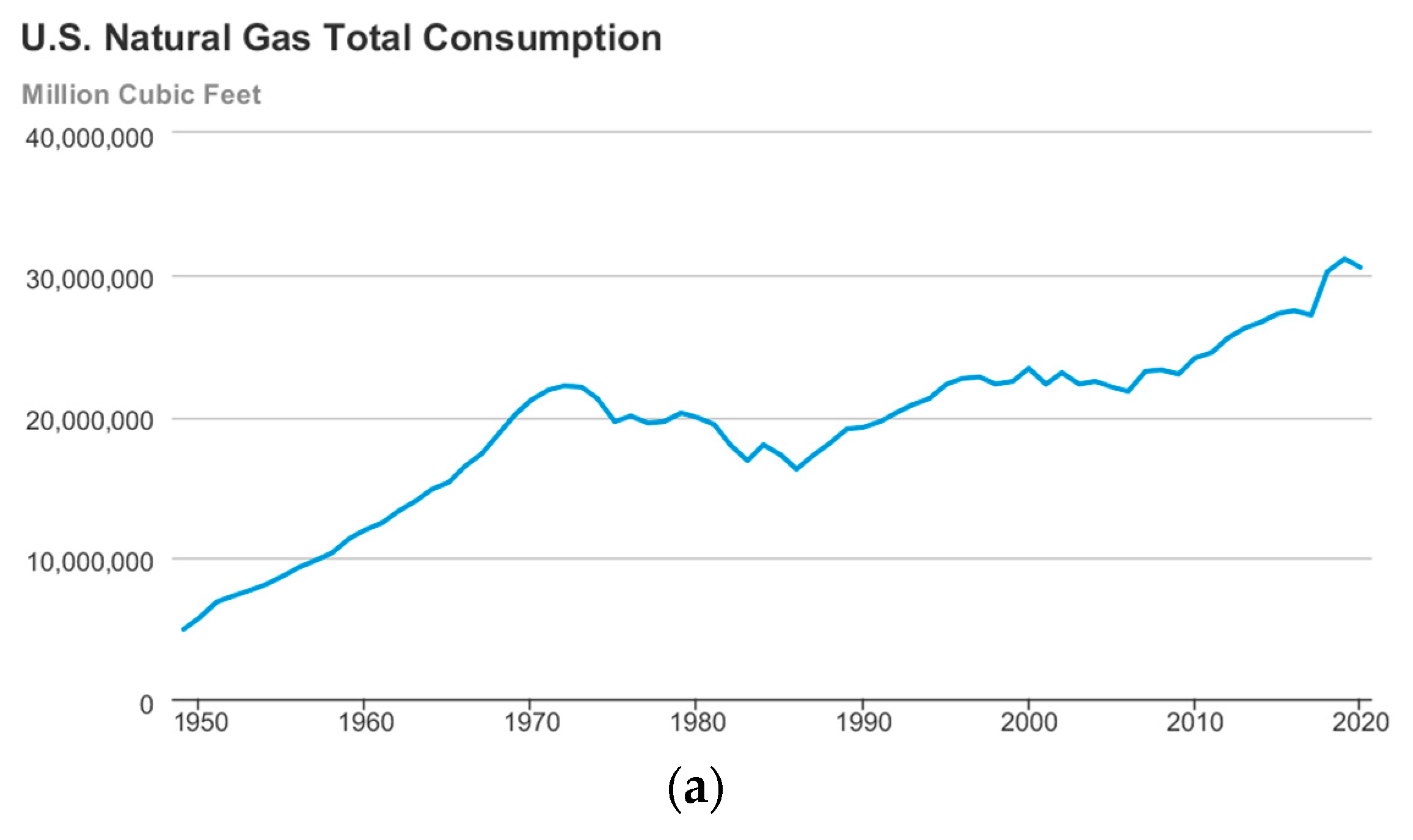
2.3. From the 1950s to the 1990s: Manufactured Gas to Natural Gas and LNG

The nation-wide organized transition from manufactured gas to natural gas occurred in the U.K., which is a good example of a government-assisted energy transition. In 1948, the U.K. Parliament passed the Gas Act and nationalized the gas industry through amalgamation. At that time, 1050 gas works existed, supplying a total of 2119 million therms to 11.3 million consumers [50]. The Gas Act also established the British Gas Council with 12 Area Gas Boards, which were responsible for arranging their own supplies and finances. The British Gas Council consisted of the 12 chairmen of the Area Boards, a Deputy Chairman, and a Chairman, whose role was to advise the government of the policies in the gas industry and coordinate different Area Boards.

A series of policies promoted by the British Gas Council significantly changed the British gas industry. For example, after the Gas Council was founded, 622 old gasworks were closed, some of the larger works were extended and linked together, and 21,200 miles of new gas mains were laid. Therefore, by 1962, the town gas production units decreased from 1050 in 1949 down to 341, of which 74 units produced around 73% of the nation’s town gas [65]. With the development of the industrial sector, the gas consumption in industry rose from 639 million therms (in 1953) to 819 million therms (in 1960).

Contrary to the wide adoption of town gas in industry, the town gas consumption in residential houses decreased from 1366 million therms (in 1953) to 1268 million therms (in 1960). This was mainly due to the increase in the price of town gas, which led the residential sector to look for alternative fuels. From 1950 to 1960, the town gas price increased by 65%; however, the electricity price only increased by 25% over the same time period. The major reason for the town gas price increase was the increasing cost and difficulty of sustaining suitable supplies of coking coal, for which the steel industry was also a major customer [66]. Facing these difficulties, the British Gas Council proposed three solutions:

• The gasification of alternative, lower-grade coal.
• Gas production from petroleum instead of coal.
• The introduction of natural gas to enrich manufactured gas.

Considering the cost and technology availabilities, the third solution became the final answer to solve the dilemma of the British gas industry. In 1953, the British Council started to work with the BP Exploration Company to find natural gas reserves all over the British Isles. The discovery of natural gas fields around the world also stimulated the British Gas Council to explore the overseas market. In the late 1950s, British Gas Council started a plan to explore the North Sea and also started to import LNG from the American Gulf Coast, Algeria, etc. [65].

In this manufactured-gas-to-natural-gas transition, combustion devices’ adaptation to natural gas posed a significant challenge. Natural gas has a volumetric heating value around twice that of town gas. Other fuel property differences, such as density, flame speed, etc., also introduced difficulties to existing combustion devices in switching from town gas to natural gas without modification. At first, it was proposed to blend other gaseous fuels into natural gas to make a fuel mixture that possessed similar burning properties to town gas while still keeping the heating value of this new fuel higher than that of town gas. This type of gas was once called “GS gas”. However, experiments showed that the old town gas appliance burners still needed modification, even with the specially made “GS gas”. Therefore, with the abundant supply and the decreasing price of natural gas, the British Council determined to take a one-step action, which was to replace the old residential appliance burners with new ones that were compatible with natural gas, instead of adopting the more expensive two-step method of exchanging both the fuel and appliances.

Starting from 1966, the appliance-conversion act took almost 10 years, with 40 million appliances from 14 million end users. By 1972, appliances from 6 million families were converted, and in the same year, the British Gas Council changed its name to the British Gas Corporation with more concentrated power authorized by the government after the 1972 Gas Act [66,67,68]. By the end of 1978, around 13.4 million town gas end-users converted to natural gas [50].

Table 4. Progress of the customer conversion to natural gas in the U.K. from the 1960s to the 1970s.

Year (April to March)	Total Customers (000s)	Annual Number Converted to NG (000s)	Cumulative Number Converted to NG (000s)
1967/68	13,210	51	51
1968/69	13,265	418	469
1969/70	13,347	1093	1562
1970/71	13,372	2029	3591
1971/72	13,390	2407	5998
1972/73	13,506	2100	8098
1973/74	13,559	2108	10,206
1974/75	13,682	1674	11,880
1975/76	13,925	1131	13,011
1976/77	14,200	329	13,340
1977/78	14,516	98	13,438

[50] shows the progress of the British gas end-users converting from town gas to natural gas.

This town-gas-to-natural-gas transition in residential homes was a huge task in British energy development history. More than 13.5 million sites had to be visited with 35 million appliances (200 million burners) and more than 8000 residential appliance models to convert. Because conversion always brings inconvenience to the residential gas end-users, the British Gas Council (British Gas Corporation after 1972) decided to provide advantageous terms for a new appliance purchase, or even offer it free of charge, when the old appliances could not be converted successfully. The British Gas Council also decided to supply the replacement parts to residential houses, so the conversion could be completed on-site. This was more efficient and cheaper compared to shipping the appliances to specific places and conducting conversion there. Figure 5 shows an on-site town gas purging using natural gas in England. To achieve this fuel conversion, not only were the training/education programs provided to technicians but the marketing strategies/advertisement of natural gas to the public were also equally, if not more, emphasized. For example, the first demonstration fuel conversion project was completed on Canvey Island, which gained public confidence in the fuel conversion. To assist the transition, the Conversion Executive was founded to coordinate among the British Gas Council, Area Boards, and the Society of British Industries, which represented the benefit of appliance manufacturers and contractors. At the same time, public relation strategies were adopted, including providing conversion handbooks/manuals, developing a better understanding of local conditions, and approaching gas end-users of different social classes/income levels using varying methods [69,70].

The successful conversion in Central London of Buckingham Palace, Parliament, the Bank of England, and Westminster Abbey acquired symbolic status in fuel conversion of the British upper class. However, different problems were encountered in other places of Britain. For example, cultural and linguistic issues became a hindering stone in the North East/West, East Midlands, etc. Specific lobby teams were developed to reach out to Asian immigrant communities, where women especially expressed greater concern for the work of fuel conversion [65]. In May 1968, a town gas explosion occurred at Ronan Point of London, which resulted in the death of four people and the injury of seventeen. The tragic accident further shook the public confidence in town gas during its campaign with natural gas. This also provided a window of opportunity for the natural gas supporters to reduce the public concern about converting from town gas to natural gas. For example, the government and the British Gas Council commissioned a report by Prof. Frank Morton of Manchester University addressing the concerns with natural gas and delivering the advantages of the fuel transition, such as reducing explosion accidents and gas poisoning [65,71].

The final cost of the fuel transition from town gas to natural gas in the U.K. was GBP 577 million in 1978 (~GBP 2.8 billion in 2021), which was less than the estimated GBP 400 million in 1966, considering inflation. However, other costs, such as writing off obsolete plants, brought the total bill to GBP 1027 million (~GBP 5.3 billion in 2021). In the April 1977/March 1978 Annual Report, British Gas Acclaimed: “The cost of the entire conversion programme was met without external subsidy of any kind” [50].

The United States experienced a different procedure of adopting natural gas in residential homes compared to the British way. Before the gas transition, the U.K. had already built a relatively mature town gas industry and gas transporting system beginning in the 1800s and then experienced an organized state-led town-gas-to-natural-gas transition by an almost monopolistic strategy developed by the British Gas Council and the British Government. However, being the world’s largest bastion of free market and entrepreneurship, the U.S. natural gas industry was developed in parallel with its manufactured gas industry due to the abundant and cheap supply of natural gas from international trades. From the late 1800s to the early 1900s, U.S. gas companies provided both manufactured gas and natural gas separately to customers depending on their specific needs. Figure 6 shows a gas company that used a wagon to advertise domestic gas usage in the early 1900s. In the U.S., the sale of natural gas exceeded that of manufactured gas in 1935. In the late 1940s, manufactured gas began to be phased out and ultimately replaced by natural gas in the 1950s [50]. However, at that time, the U.K. had not yet started the conversion project.

The first recorded usage of natural gas in the U.S. was from Fredonia, New York, in 1821. Local residents used logs and later lead pipes to transport the gas to nearby houses for illumination [72]. This first known natural gas practical application in New York was four years before the foundation of the New York Gas Light Company. However, in the United States, from the discovery of natural gas in 1821 to its sale exceeding manufactured gas in 1935, enormous volumes of natural gas were flared due to the lack of local usage or in hopes that oil might be lying under the gas. It was estimated that around 76 trillion cubic feet of natural gas were wasted from the early days of the oil industry to the late 1940s [50]. In the late 1800s, the natural gas industry started to thrive due to the development of pipeline transportation technology and the discovery of natural gas on U.S. land. In 1883, the Penn Fuel Company started to distribute natural gas by pipeline to customers in Pittsburgh’s East Liberty and Lawrenceville neighborhoods from Haymarket Well [73]. The first long-distance pipeline (217-mile/14- to 18-inch) transporting natural gas was completed in 1925 by the Mongolia Gas Company of Texas from northern Louisiana to Beaumont, Texas [74]. In 1947, the original oil-transporting pipelines (the “Big Inch” and the “Little Big Inch”) connecting Texas and the U.S. East Coast converted the fuel to natural gas after they were sold to Texas Eastern Transmission Corporation after the Second World War [75]. By 1966, natural gas pipelines were lying in every one of the lower 48 states. The natural gas consumption by American residential end-users also increased dramatically, as shown in

Table 5. U.S. domestic natural gas consumption from 1945 to 1977.

Year	Total Customers (Millions)	Total Consumption (Trillion Btu)	Average Consumption (Million Btu/Customer)
1945	18.6	775	41.6
1950	22.1	1384	62.6
1955	26.3	2239	85.2
1960	30.4	3188	104.8
1965	34.3	3999	116.5
1970	38.1	4924	129.2
1975	40.9	4991	121.9
1977	41.7	4946	118.7

[50].

The natural gas consumed in the U.S. was not only from domestic sites but had also been also imported from Canada, Mexico, or Algeria in liquid form since the 1950s. The natural gases on the energy market possess distinctive properties depending on their sources.

Table 6. Variation in composition of natural gas in the U.S. market.

Component	Volume (%)
	Mean	Standard Deviation	Minimum	Maximum
CH4	93.0	5.5	73	99
C2H6	3.0	2.6	0	13
C3H8	1.0	1.4	0	8
C4H10	0.5	1.0	0	7
C5H12	0.1	0.3	0	3
C6H14	0.1	0.1	0	1
N2	1.5	2.9	0	17
CO2	0.5	0.5	0	2

[76] summarizes the components and their relative abundance in investigated natural gases on the U.S. market. As shown, the major functional specie of natural gas is methane, together with some higher hydrocarbons. The diluents are usually nitrogen, carbon dioxide, or a trace of oxygen. It should be noted that the contents of the natural gas in Table 6 are only the ones investigated. Natural gas from non-investigated resources might extend the percentage of these species into a larger range.

With natural gas species varying from different sources, the natural gas either mined or purchased by the U.S. gas utility companies also varied significantly. Lacking the unified national natural gas quality regulation, gas companies in the U.S. developed their own standards for the natural gas species, such as the heating value and sulfur contents.

Table 7. Natural gas quality standards adopted by gas companies of the United States.

Gas Company	Heating Value (Btu/scf)		Water Content	Various Inerts			Hydrogen Sulfide (H2S)
	Min	Max	Lbs/MMscf	CO2	O2	Total Inerts	(Grain/100 scf)
SoCalGas	970	1150	7	3%	0.2%	4%	0.25
Dominion Transmission	967	1100	7	3%	0.2%	5%	0.25
Equitrans LP	970	-	7	3%	0.2%	4%	0.3
Florida Gas Transmission Co.	1000	1110	7	1%	0.25%	3%	0.25
Colorado Intrastate Gas Co.	968	1235	7	3%	0.001%	-	0.25
Questar Pipeline Co.	950	1150	5	2%	0.1%	3%	0.25
Gas Transmission Northwest Co.	995	-	4	2%	0.4%	-	0.25

[77,78] shows the natural gas quality regulations of some gas utility companies in the United States. Some of these regulations were modified every few years. For example, in 2019, SoCalGas decreased their natural gas minimum heating value from 990 Btu/scf to 970 Btu/scf [77].

Fuel-interchangeability studies in the United States started from the manufactured gas era and are still underway for natural gas from different sources. Although lacking a government-led uniform gas-transition strategy like the U.K., early records of fuel-interchangeability studies being conducted on manufactured gases and natural gas in the late 1800s and early 1900s from some U.S. institutes are noted.

In the late 19th century, the large cost increase in gas-making materials resulted in frequent manufactured gas price increases in the United States. In some localities, the gas price increase compelled a decrease in standards of quality. At that time, natural gas production was not as abundant as today. Therefore, a variety of gases were available on the market, including natural gas, manufactured gas, or artificially lower-standard manufactured gas. As a result, the investigation of residential burner mechanisms operating on multiple gases was conducted. The American Gas Association started to work on the project of improving the gas-utilization efficiency, which was one of its earliest tasks after its foundation in 1918. Meanwhile, the engineering section of the U.S. Bureau of Standards started to investigate the design and operation of atmospheric burners, which were, and still are, commonly adopted in residential appliances. Through these studies in the early 1900s, a better understanding of residential appliance burner working principles was obtained [79]. Later in 1932, other than the burner efficiency, reducing emissions from combustion such as carbon monoxide also became a consideration in residential burner design [80]. Therefore, more detailed residential burner optimization started to be conducted considering efficiency, flame characteristics, carbon monoxide emission, etc. [81]. The test setup for residential burners is shown in Figure 7.

One of the most successful fuel-interchangeability studies on residential burners was conducted by the American Gas Association started in 1927. This six-year-long project was called Mixed Gas Research, which conducted around 175,000 individual tests involving more than 250 gases. In 1936, AGA released their general formula, the “AGA Index C”, to represent the gas interchangeability, where C = the index of change in performance of appliances. The $\mathrm{AGA} \mathrm{Index} \mathrm{C}=\mathrm{H}/\sqrt{D}$, where H is the gas heating value and D is the gas-specific gravity [82]. This index is nowadays referred to as the Wobbe Index, which is widely adopted around the world in gaseous-fuel interchangeability studies. Not soon after, researchers realized that a single Wobbe Index was not enough to predict all the combustion behaviors. Therefore, more indices regarding flame blow-off, flashback, yellow tip, and so on were developed to examine the performance of residential burners. From the perspective of technical development, these preliminary fuel-interchangeability studies in the U.S. since the 1900s assisted the transition from manufactured gas to natural gas. The research results also benefited the historical energy conversion of the U.K. in the 1950s.

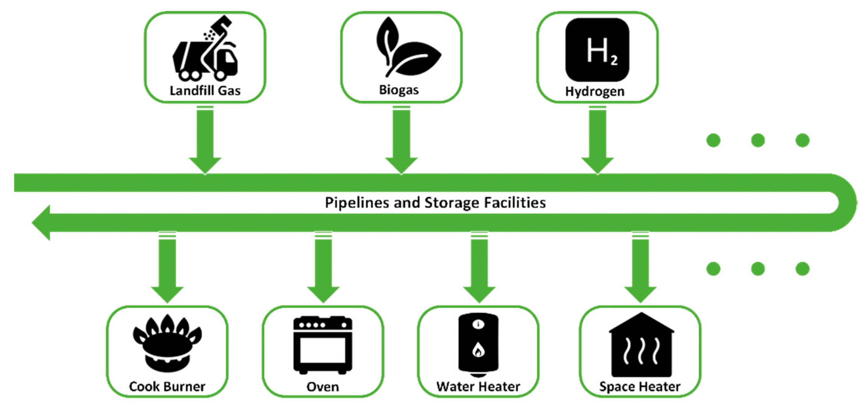
2.4. Since the 1980s: Renewable Gases

With the depletion of natural gas reserves and the urgency to reduce carbon emissions to combat climate change, replacing natural gas with renewable gases in pipelines has been of interest not only to fossil-fuel-dependent countries but also to all of human society. Although many complexities remain to be sorted out, reducing carbon emissions by replacing fossil fuels with renewable energy is a strategy that has international consensus, as evidenced by the endorsement of the United Nations Framework Convention on Climate Change in 1992 [83]. For the residential sector, one of the most effective ways of adopting renewable energy is to replace pipeline natural gas with renewable gases [84], as shown in Figure 8. The benefits of adopting renewable fuels in natural gas pipeline infrastructure include:

• Reducing carbon emissions, thus combating climate change.
• Extending the gaseous fuel from singular fossil fuel sources to more renewable sources, such as biogas or hydrogen.
• Obtaining energy security by alleviating the influence of natural gas price fluctuation.

2.4.1. Biogas

Biogas can be produced from various sources, including wood and agricultural products [85,86,87], landfill waste [88,89,90], and sewage [91,92,93]. Although biogas production sources may vary, the functional part in different sources is mainly biomass. The biogas sources influence the contents of biogas significantly, and

Table 8. Typical biogas contents.

Species	Units	Biogas
		Sewage Gas	Agricultural Gas	Landfill Gas
CH4	%	66–75	45–75	45–55
CO2	%	20–35	25–55	20–30
CO	%	<0.2	<0.2	<0.2
N2	%	3.4	0.01–5	10–25
O2	%	0.5	0.01–2	1–5
H2	%	trace	0.5	0.0
H2S	mg/N·m3	<8000	10–30	<8000
NH3	mg/N·m3	Trace	0.01–2.5	trace
Siloxanes	mg/N·m3	<0.1–5.0	trace	<0.1–5.0

[94] shows typical biogas contents.

The variation of biogas species is not only related to biomass sources but also to gasification technology and procedures. The two major species in biogas are methane and carbon dioxide. Other common fuel species such as carbon monoxide and hydrogen are present at much lower levels. Other species in raw biogas include nitrogen, oxygen, ammonia, hydrogen sulfide, etc. However, some of these trace gases might be detrimental to pipeline or combustion devices through direct contact or combustion. Therefore, before blending biogas into a pipeline or supplying it to combustion devices, the gas needs to be purified or processed to be “upgraded” to meet certain standards.

The major functional species in biogas is methane, which is usually called biomethane due to its production source. The first known large-scale project for blending biomethane into the natural gas grid was in Moenchengladbach, Germany. The sewage gas plant had a raw gas capacity of 400 m³/day and injected around 20 million m³ of purified biogas (biomethane) into the local gas grid from 1982 to 1996 [95]. This practice was later followed by the other countries in Europe [96], as well as the U.S. [97], Canada [98], Japan [99], etc. [100,101].

2.4.2. Renewable Hydrogen

Hydrogen has long been touted as a long-term solution for carbon reduction, and hydrogen from renewable sources has increasingly gained attention [15,102,103]. Hydrogen is the most abundant element in the universe and is also a carbon-free combustible fuel. Besides combustion, hydrogen can also be readily used in other applications, such as fuel cells, industrial refineries, or ammonia production for agricultural fertilizers. Moreover, being the lightest element, hydrogen has a much higher heating value on the mass base compared to fossil fuels, which also makes it a competitive energy carrier in addition to being a fuel. Therefore, storing renewable energy (solar, wind, etc.) into hydrogen, transporting hydrogen through pipelines, or directly blending hydrogen into the existing natural gas infrastructure can be an effective way to achieve renewable-energy-adoption and carbon-reduction goals.

Renewable hydrogen as a fuel supply and an energy carrier to power the world is far from being a new idea. The notion of using hydrogen from electrolization dates back 100 years. In 1923, the famous British scientist J.B.S. Haldane published the book Science and the future [104], which noted, “The country (U.K.) will be covered with rows of metallic windmills working electric motors which…will be used for the electrolytic decomposition of water into oxygen and hydrogen. These gasses will be liquefied, and stored in vast vacuum jacketed reservoirs, probably sunk in the ground”. Considering hydrogen as a highly condensed energy carrier, Haldane also mentioned that hydrogen “will enable wind-energy to be stored, so that it can be expended for industry, transportation, heating, and lighting, as desired”. Compared to coal and petroleum, which were fuels widely used in the U.K. in the 1920s, Haldane also mentioned the environmental benefit of using hydrogen as “no smoke or ash will be produced”. Despite the promising utilization of hydrogen, Haldane expressed his concerns regarding the capital investment by saying “the initial costs will be very considerable”. As natural gas storage and transporting technology have developed, the current cost of utilizing hydrogen in existing natural gas systems should be much lower than in 1923, when Haldane made this prediction. Today, hydrogen has already found a wide range of applications in industry and transportation and is being considered for residential heating.

Beyond Haldane’s suggestion of utilizing wind power, technologies are now available to generate renewable hydrogen from other sources, including renewable feedstocks [105], solar energy [106], nuclear power [107], or directly from water electrolysis by renewable grid power (P2G, Power to Gas) [108]. Hydrogen is categorized by color coding according to various generation sources. Black or brown hydrogen uses black (bituminous) or brown (lignite) coal in the hydrogen-production process, which is the most environmentally damaging method as both the carbon dioxide and carbon monoxide generated during the process are not recaptured. Gray hydrogen is the most common form used currently and is generated from methane or natural gas through steam reformation. Hydrogen is labeled blue when the carbon generated from steam reforming is captured and stored (CSS). Green hydrogen is produced from renewable energy sources, such as solar or wind power, using water electrolysis. Pink hydrogen is created through the electrolysis of water by nuclear energy. Hydrogen has already been integrated into pipeline infrastructure, as previously discussed. We can recall that Britain once had a high percentage of hydrogen (around 50 vol%) in their town gas for over half a century. Therefore, blending hydrogen into our existing pipeline should not be as difficult as the very early adoption of hydrogen in the manufactured gas era. However, since current pipeline infrastructures around the world are mainly designed for natural gas, blending hydrogen into the natural gas system warrants some technical considerations regarding the fuel property differences between natural gas and hydrogen.

Hydrogen has a much lower density compared to natural gas, and its high flame speed and wide flammability range limit its percentage in the current natural gas infrastructure. Therefore, the hydrogen utilization in the natural gas grid is still in the demonstration stage, and the hydrogen-blending percentage is still on the lower end (generally under 10–20 vol%). Reference [109] lists the demonstration projects of hydrogen injection into existing natural gas pipeline infrastructure.

Before trying to increase the percentage of hydrogen in residential pipelines, multiple sectors need to be considered, including pipeline material, sealing, and compression system adjustment. From a combustion perspective, the ability of end uses, such as residential appliances being able to safely operate on hydrogen/natural gas mixtures, is important to assess. Further, what adjustments should be made to existing appliances to increase their tolerance level of hydrogen? Ironically, the process may look like a reversal of the retrofit program undertaken in the U.K. to adapt appliances to switch from town gas to natural gas.

Some preliminary studies have been conducted and are still ongoing in several countries. In the 1970s, Pangborn et al. [110] projected technical considerations on a typical residential atmospheric burner (designed for natural gas) operating on hydrogen. In Europe, the NATURALHY project was initiated in 2004, which aims to prepare for the hydrogen economy. After the start of this project, De Vries et al. conducted both theoretical and experimental research to investigate the feasibility of using hydrogen in our current natural gas appliances. However, these studies mainly stayed on either atheoretical level or only tested on fundamental burners [111,112,113,114].

In 2018, Jones et al. conducted tests on a commercial cooktop burner designed for natural gas and successfully injected 34.7% hydrogen into the cooktop burner without inducing flashback [115]. Around the same time, the California Energy Commission (U.S.) sponsored the University of California, Irvine, to conduct a more comprehensive study on existing natural gas appliances operating on natural gas/biogas and natural gas/hydrogen mixtures. Using both experimental and numerical methods, this study investigated the combustion performance of multiple commercial and residential appliances, including cooktop burners [116,117,118], oven burners [119], water heaters [120,121], room furnaces [122], etc. The investigated combustion performance included flashback/blow-off limits, ignition behavior, burner temperature, emissions (CO, UHC, NO, NO₂, N₂O, NH₃), combustion noise, efficiency, etc. In 2019, the University of Zaragoza worked with the BSH Home Appliances Group in Spain on reaction mechanism simplification to generate numerical models to predict combustion behaviors of appliances operating on hydrogen-rich fuel [123]. Additionally, in 2019, an appliance test project was initiated by E.ON, which is one of the largest companies in Europe working on P2G programs. E.ON planned to raise the hydrogen percentage in the natural gas pipeline grid to as much as 20% in Schopsdorf (Germany). To help achieve this goal, 400 commercial and residential appliances were selected for tolerance tests [124]. These activities are summarized in

Table 9. Tests on residential appliances operating on hydrogen-enriched natural gas.

Organization	Starting Time	Appliances/Burners	Description	References
Gas Technology Institute, U.S.	1977	Atmospheric burner	Provided technical considerations of appliances operating on hydrogen-rich natural gas.	[110]
DNV GL Oil & Gas/University of Groningen, Netherlands	2004	Fundamental aspirating burner	Conducted fundamental analysis on natural gas/hydrogen mixture properties and conducted experiments on a Bunsen burner.	[111,114]
Swansea University, U.K.; King Saud University, Saudi Arabia	2018	Cooktop burner	Conducted experiments on a cooktop burner operating on over 30 vol% hydrogen.	[115]
University of California, Irvine, U.S.	2018	Cooktop burner, oven burner, room furnace, water heaters, etc.	Conducted experiments on multiple appliances and tested multiple performances (ignition, emissions, burner temperature, etc.) of various appliances operating on hydrogen/natural gas mixtures.	[116,122]
University of Zaragoza, BSH Home Appliances Group, Spain	2019	Cooktop burner	Developed simplified reaction mechanism to simulate the combustion performance of a cooktop burner.	[123]
E.ON/DVGW, Germany	2019	Various appliances	Around 400 residential appliances were tested while operating on hydrogen/natural gas mixtures.	[124]

.

As mentioned, hydrogen was already integrated into gas pipeline systems during the manufactured gas era. Replacing part of pipeline natural gas with renewable hydrogen is thus plausible. Technical considerations regarding hydrogen compression, leakage, pipeline material, etc., can draw lessons from the manufactured gas era. To increase the hydrogen tolerance level of current natural gas appliances, insight can also be obtained from the designs of manufactured gas burners. However, it should be noted that, since the manufactured gas era, modern residential burner designs have more requirements. Besides safety concerns, other requirements such as low emissions, high efficiency, ease of operability, longer lifetime period, and visual appeal must be considered in modern residential appliances design. As a result, while “reversing” the transition from manufactured gas to natural gas can give guidance, shifting from natural gas to natural gas/hydrogen mixtures and perhaps ultimately 100% renewable hydrogen will require more effort.

2.5. Summary

When it comes to fuel consumption, technology advancement, or emission control, the power generation, industry, and transportation sectors are usually first in line. The residential sector, which is most related to our daily lives, is usually overlooked. However, as discussed above, nearly every energy transition in human history was either initiated by or highly influenced by the residential sector. From fuelwood to coal, then to oil and different gaseous fuels, industry consumed large amounts of resources, which led to higher prices being less affordable to residents. The old fuel depletion due to the industrial sector drives the residential sector to seek less-expensive alternative fuels. For large fuel-consumption sectors such as industry, when the benefit of adopting the new fuel can balance out with the cost of throwing out their old fuel-consumption devices, the fuel transition will occur in these high-energy-consuming sectors. Therefore, in the energy transition, industry usually has a time delay in adopting the new fuel due to the capital investment required for their devices to adapt to the new energy source. However, the residential sector is more flexible and price-sensitive due to the relatively low capital investment in appliances and more flexibility in consumer adoption/replacement tendencies. Examples besides appliances include electric vehicles, rooftop solar, IOT devices in the home, etc. This places the residential sector in the pioneering position when energy transition occurs. Therefore, investigating the energy transition in the residential sector is not only beneficial to the residential sector study itself but can also help foresee future fuel transitions in other energy-consuming sectors.

Fuel transitions have also been assisted or promoted by other factors, such as government policies and stricter emission regulations. For example, after the Great Smog of London in 1952, the necessity of replacing coal with cleaner fuels was finally widely accepted by the U.K. society. The Clean Air Act 1956 passed by the Parliament of the U.K. was principally in response to the smog, which accelerated the transition of the U.K. from coal consumption to gas adoption. This successful fuel transition is a great example of how rational policy can play a leading role in energy transitions and emission control.

Yet, it is clear that air pollution problems in London were evident well before the 1950s. People were suffering from respiratory deceases due to coal combustion, and church roofs were being damaged by the high sulfur content of coal ashes in the smog hundreds of years ago before the London Smog in 1952. Numerous policies were put in place before the Clean Air Act 1956, but they all failed in some manner. The successful adoption of the Clean Air Act of 1956 is usually attributed to the human reflection and awakening after the deadly tragedy of the 1952 London Smog, which finally ended the coal era in London. Under this government-led energy transition, another critical factor that helped facilitate the transition was the large amount of natural gas discovered in the North Sea in the 1950s. While this discovery did not have the public impact of the London Smog episodes, it enabled Europe to use cheaper and cleaner natural gas than coal. As a result, one must ask: Did the discovery of cheap natural gas or the Clean Air Act 1956 end the smog tragedy? If the Clean Air Act were proposed in the Victorian era, would it be as successful as the one in 1956, or would it have been another failed policy like its predecessors? It is apparent that transitions require many factors to properly align in order for action to occur.

The discussion above touches on general trends in fuel transition. Of course, not all countries in the world were participating in this transition or experiencing the same processes. Even in the U.K. and the U.S., not every city was participating in the energy transition. For example, while the U.S. transitioned into the natural gas era more than 50 years ago, around 10% of U.S. residential houses still use fuelwood or coal for residential heating. Other countries may not follow this procedure or may skip several steps. For example, some developing countries in Africa or Asia continue to use biomass combustion for residential heating, including dry bushes, tree leaves, and residuals of crops, which corresponds to a fuel-consumption stage even preceding the fuelwood era in the developed world. However, these later-developed countries may be able to skip some energy-transition steps and directly enter the renewable gas era by adopting biomass gasification technologies if assisted by the developed world. Certainly, the world must adopt renewable resources in the near future to help combat climate change.

3. Domestic Gas Appliances vs. Electric Appliances

3.1. Lighting Market

A current debate is ongoing relative to transitioning from gas fuel combustion appliances to those that run on electricity [125,126]. Such debates between residential devices operating on electricity vs. gas fuel have been taking place since the introduction of technologies that enabled widespread availability of the electric infrastructure in the 1870s. The first battlefield between the gas and electricity industries was in the lighting market.

Before the 1870s, the lighting market was mainly dominated by kerosene and gas lighting. However, as shown in

Table 10. Lighting system development path since the 1870s.

Year	Event	References
Early 1870s	Introduction of the electric dynamo posed a competitive threat to kerosene and gas lighting.	[127]
1877	Carbon arc lamp was first used in Paris in May 1877, which triggered the interest of London.	[128]
	Dr. Carl Auer von Welsbach of Vienna invented the incandescent gas light mantle. Welsbach established the first factory to make gas mantles in London in 1877.	[53,129]
1878–1879	On 14 December 1878, the Holborn Viaduct electric lighting was switched on in London. Afterward, four circuits, each with four lamps, were powered by a 20-horse-power Robey steam engine that drove a Gramme alternator and exciter. However, the experimental lighting was shut down on 9 May 1879. The city engineer reported that the cost was 3.75 times that of gas.	[128]
1879	Edison invented the long-life light bulb and applied for a patent.	[130,131]
1882	Electric Lighting Act (U.K.) led to the establishment of electricity undertakings on a statutory basis, but the high cost of electricity hindered the wide application of electric lighting.	[132,133]
1890s	Gas mantle started to be widely used for streetlights.	[133]
1900s–1910s	By the early 1900s, the cost of electric lighting was becoming closer to that of gas. However, only the wealthy could afford to wire their houses until the 1910s.	[21]
After 1910s	World War I resulted in coal shortage and the coal gas quality fluctuation, which gave a chance for electric lighting popularization. After World War II, the power-generation technologies and electric grid were rapidly developed, which brought down the electric lighting price, and electric lighting found wide applications not only in street lighting but also in residential houses.	[134]

, electrical systems started to be introduced at this time, offering a possible alternative for lighting. In 1877, the first electric arc lamp was tested on the street of Paris, which triggered interest in adopting electric lighting in Europe. In 1878, London started to perform tests on electric streetlamps; however, this project was ended a few months later due to the high cost of relatively scarce electricity. While the electric lighting systems were being tested in the 1870s, the gas industry invested in high-efficiency gas lamps to compete with electric lamps. In 1877, Dr. Carl Auer von Welsbach opened the first factory in London to produce incandescent gas light mantles, but the gas mantles did not gain much popularity until the 1890s. From the 1870s to the 1880s, electric lighting technologies advanced rapidly, including the invention of the light bulb by Thomas Edison. The U.K. government passed the Electric Lighting Act in 1882 to promote electric lighting adoption. Ironically, the market share of electric lighting remained limited. In fact, the gas mantle lighting system started to take market share back from electric lighting due to electricity price fluctuations.

In the time around World War I, electric lighting started to gain favor due to shortages in coal gas and related price fluctuations. As the technologies for electricity generation and transport matured after World War II, electricity prices dropped significantly, and electric lighting dominated all market sectors as it still does today.

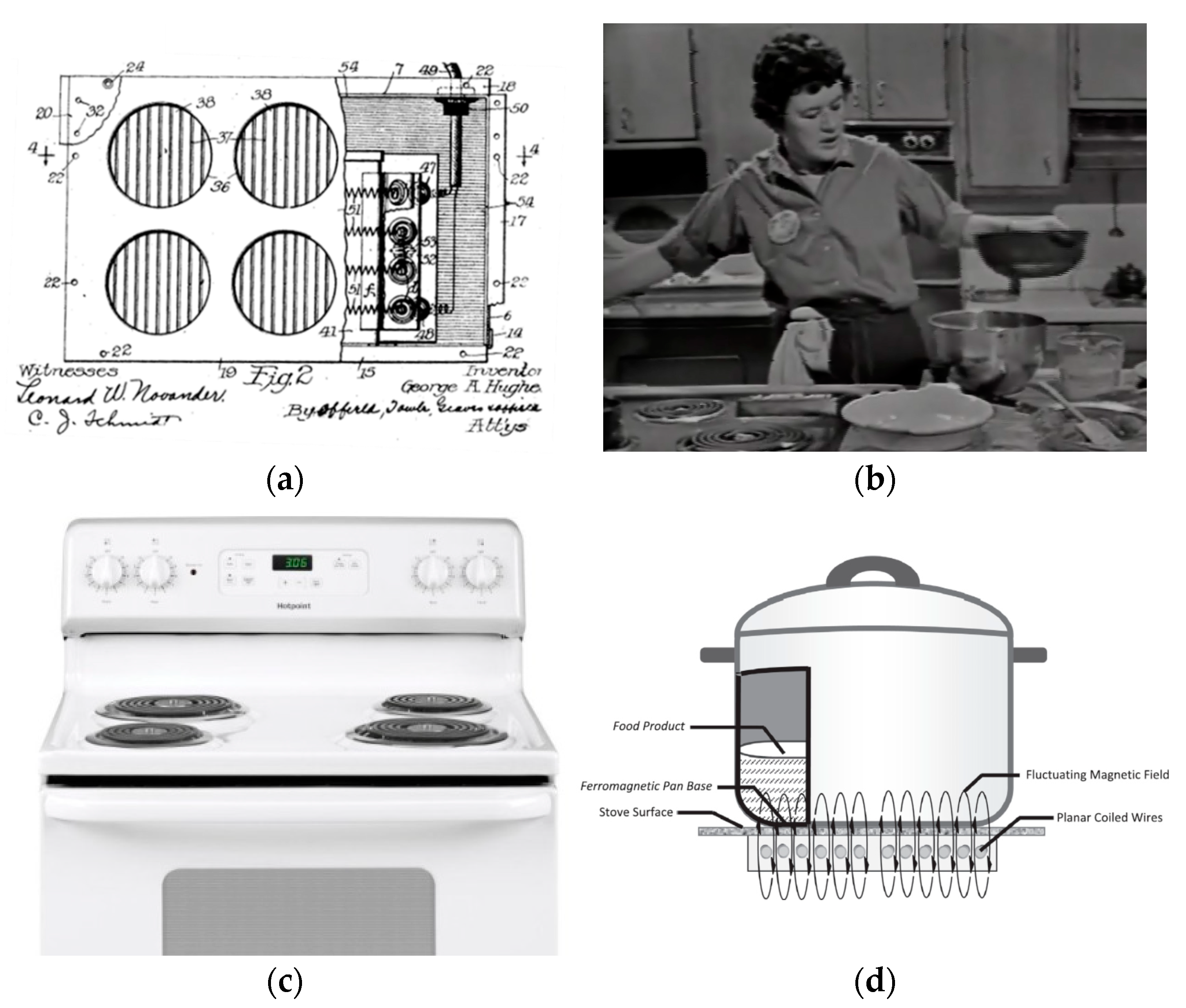
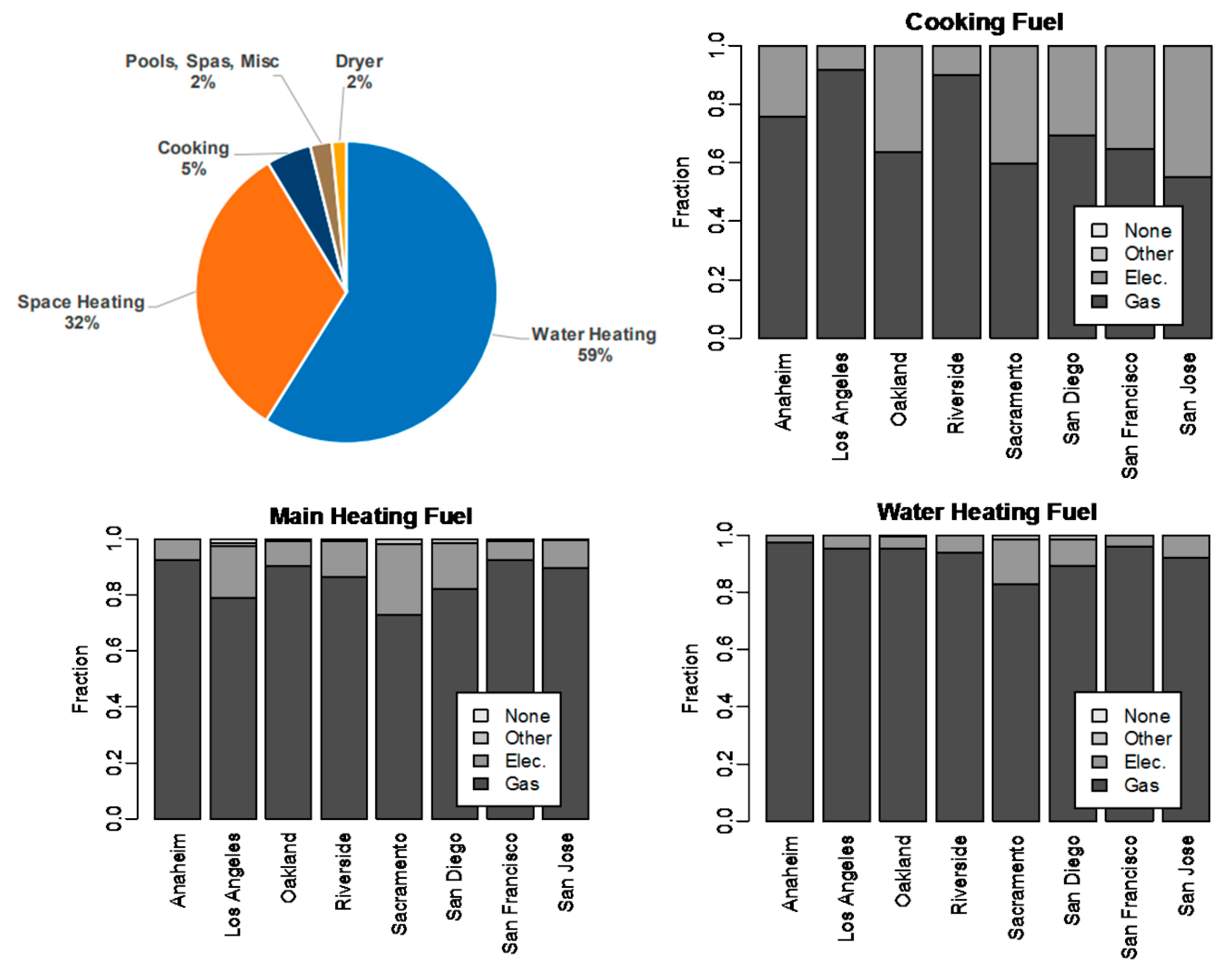
3.2. Cooking, Air/Water Heating, and Other Applications

The majority of energy consumption in residential homes is associated with lighting and heating. Heating includes cooking, air (space) heating, water heating, and other small applications such as irons, dryers, and kettles.

It is believed that the first successful commercial cooking range was from the United States. In 1915, George A. Hughes from Iowa applied for a patent on his invention—an electric range with simple heating element wires set in clay bricks [135]. In 1918, Hughes merged his company with General Electric. In the 1920s, electric appliances started to appear in residential homes in both the U.S. and Europe due to the thrust of appliance manufacturers such as General Electric, Westinghouse, and Siemens [136,137,138]. Figure 9 shows the evolution of the appearance of electric cooking ranges. Not much change is evident even over 100 years. When it was first developed (as shown in Figure 9a), the electric wires were in parallel; then, they were optimized into coil shapes to promote better contact and support to the cooking utensils. Figure 9b shows an image from the TV show “The French Chef” with Julia Child cooking with electric stove tops in the early 1960s. Even today, the basic electric stove tops remain similar, as shown in Figure 9c.

In recent years, another type of electric cooking technology, induction, has gained popularity. Induction cooking technology is based on the principle of static magnetic fields. Alternating current flowing through an induction coil generates a magnetic field with changing polarities. This alternating field “induces” eddy currents that are trapped within the steel material that forms the base of the pan and transfers heat to the food it contains. The induction cooking surface provides a “clean” appearance and higher efficiency compared to traditional electric stoves. However, it is generally more expensive and also requires specific cooking pots and pans that are made of magnetizable materials.

Compared to gas cooking appliances, electric cooking appliances usually have higher operating efficiencies. In the U.S., the average efficiency of gas stoves is around 40%, which is significantly lower than the 74% efficiency of their electric competitors [141]. In Europe, electric cooking appliances have similar efficiencies as that of the U.S., but gas cooking appliances have a higher range of efficiency, from 52% up to 69% [140].

However, despite their early appearance in the market and evolution over 100 years, electric appliances do not dominate the current residential market. The high price and maintenance fee of electric appliances and electricity itself is part of the reason. Additionally, when considering the “source to pot” efficiency, it is evident that many losses occur. As shown in Figure 10, the total system efficiency of utilizing electric appliances not only includes the appliance efficiency itself but also includes the efficiency of electricity production and transmission process. Currently, most of the electricity in the world is generated from fossil-fuel-based power plants, whose highest efficiency is around 60% [142]. Further, according to the U.S. EPA, in 2019, the average efficiency of fossil-fueled power plants in the United States was only 36% [143]. Figure 10b compares the efficiencies of cooking appliances using multiple energy sources. As shown, even if the end-use efficiency of electric cooking appliances is assumed to be relatively high at 80%, the total efficiency is only around 18%, which is much lower than the natural gas appliance efficiency of 45%.

Figure 10b shows an efficiency comparison of different types of residential cooking appliances. Cooking applications exhibit smaller variations in system efficiency due to the large energy loss in the cooking process. However, when it comes to air-heating and water-heating appliances, the gas appliance total system efficiency is higher than the electric competitors. The operating efficiency of residential gas-fired air furnaces is typically greater than 80% [122,144]. Tankless water heater efficiencies are typically greater than 90% [120]. With the large gap between electric appliances and gas appliances in the water-heating and space-heating applications, it does not seem likely that energy savings will result from electrifying residential homes.

One possible advantage of electrifying residential houses is shifting the emissions of greenhouse gases and other pollutants such as CO/NO_X to the electricity generating sector, which is mainly power plants. It is relatively easy to control the emissions from a few power plants rather than from millions of households. However, as electrification increases, more demand for electricity will occur, which will likely drive prices up. Further, with the higher penetration of clean but intermittent renewable energy sources, such as solar and wind, electrifying residential homes may add extra dispatchable fossil-fuel-based power and/or expensive energy-storage devices. This might increase the total greenhouse gas emissions, which is quite the opposite of what is intended. Combined with the decrease in electric appliance efficiency compared to gas-fueled appliances, an even greater impact on the electrical system results again, foreshadowing higher electricity prices.

Figure 11a shows the U.S. natural gas consumption in the residential sector from 1949 to 2020. After the 1970s, natural gas consumption reached a plateau. Starting in the late 1980s, natural gas consumption showed a slowly increasing trend, with a small surge before the COVID-19 pandemic. As shown in Figure 11b, in 2019, about 16.1% of natural gas was consumed in the residential sector, which is the third-largest percentage after power generation and the industrial sector. In the near term, if renewable power supplies are not available, electrification of the residential sector will require this 16.1% to be provided by power generation. As shown in Figure 11c, this electrification will increase the total natural gas consumption by 25%, and the natural gas consumption percentage in the electricity generation sector will increase from 36.3% to 59%, if not assisted by renewable electricity supply. The total U.S. natural gas consumption will also increase by 16% up to more than 36 M cubic feet per year. This assumption is relatively conservative since the efficiency difference of the cooking appliances in Figure 10b is used to predict the system efficiency decrease in the residential sector. If considering the larger system efficiency gap of water heaters and air furnaces between using gas and electricity, even more natural gas would be consumed in the electric-power-generation sector.

The challenge for this transition is significant. The State of California in the United States is one of the most ambitious regions in the world, promoting renewable energy and reducing carbon emissions. In September 2018, California passed Senate Bill 100, setting a world-leading precedent by committing to 100% renewable electricity by 2045 [146]. Together with the renewable electricity goal, California also aims to electrify home appliances [11,147,148,149]. Yet, even with these actions, a significant time lag in available renewable electricity resources is likely, which warrants an approach with diverse sources in the near term. Figure 12 shows the natural gas consumption by different appliances in residential homes of California (U.S.), which reveals that water heating, air (space) heating, and cooking dominate the use of natural gas [150]. The column charts show the energy sources for these three sectors in large representative cities of California. More than 60% of the households in California use natural gas to cook, and more than 80% of the households use natural gas to heat water and space [151]. Based on the current status, electrifying Californian residential homes will face great challenges. The increased demand for renewable electricity will likely increase utility costs for consumersm, which may hinder the progress of electrifying residential homes. It is estimated by the California Building Industry Association (CBIA) that it could cost (1) USD 7200 per household to upgrade wiring and electrical panels to purchase new appliances, (2) USD 877 higher annual utility costs per household, and (3) an overall cost increase of USD 4.3 to USD 6.1 billion per year in California [152]. It should be noted that when the U.K. was undergoing the transition, the cost of replacing appliances across the country was covered by the government-owned British Gas Council. For countries with a free market today, the cost of converting gas appliances to more expensive electric appliances is less likely to be covered 100% by electricity utility companies.

It is apparent that electrifying residential homes must be assisted by renewable energy sources. This is exacerbated by the fact that current renewable electricity availability is far less than that needed to replace the fossil fuel power supply. Governments around the world are trying to establish policies to increase the percentage of renewable electricity generation.

The discussions above focused on energy consumption and cost concerns. However, another important challenge is people’s acceptance of using electric over gas appliances. If not considering possible higher electricity bills, people may have less concern for adopting electric appliances for heating air and water because they cannot feel the difference between gas and electric appliances from the heated air or water. However, when it comes to cooking, a clear preference of gas over electricity is evident. In 2014, a survey was conducted among 100 professional chefs across the United States, and 96 reported they prefer using gas burners. The reported advantages of using gas stoves include fast response speed and controllability, high adaptability of cookware, simple cleaning, and inexpensive maintenance [153]. Advantages of gas over electric cooking appliances have been highlighted since the introduction of electric cookstoves 100 years ago. Given the limited advances in either gas or electric cooking appliances in past decades, sentiment regarding the preferred fuel has not changed. Even though Julia Child used electric stoves on the TV show in the 1960s, it still did not popularize them enough to displace gas ranges. It is also interesting to note that while Julia Child used electric appliances on TV, she actually had a gas stove in her own house [154]. The reason she used the electric stove on TV was more of a sponsor issue. When WGBH planned to shoot the scene at the demonstration kitchen of the Boston Gas Company, they learned that the kitchen was dismantled in 1962. As a result, the Cambridge Electric Light Company offered to provide their electric demonstration kitchen for the “The French Chef” [155]. Moreover, General Electric was the co-sponsor for this show and provided the electric stove. Besides her personal use of a gas range, in published letters to her book editor and friend Avis Devoto, it was also clear that Julia Child strongly preferred cooking with gas [156]. It should be noted that the promotion of any specific energy form might have been motivated by the pursuit of profits.

3.3. Summary

It took less than 40 years for electricity to take over residential lighting since the first arc lamp was lighted in 1877 on a street in Paris. However, more than 100 years have passed since electric appliances for cooking and heating were first introduced, and they still remain a small portion of the heating appliances market. This might be caused by the intrinsic disadvantage of electric appliances for cooking and heating. In reality, people do not necessarily need electricity to heat food, air, and water.

For lighting systems, electricity has the intrinsic advantage of converting to light with high efficiency. However, combustion converts most of the energy in the fuel into heat, which is what is needed for cooking and domestic heating. If heat is required to first be converted into electricity in power plants before the output electricity is transported into residential homes, it needs to be converted to heat again. The energy loss in this process is significant.

Currently, the major consideration of electrifying residential homes is to reduce emissions from the residential sector and allocate the emissions into the power-generation sector. As discussed above, due to the efficiency loss in this appliance-conversion process, there might be an increase in greenhouse gas emissions if this conversion is not assisted by the high uptake of renewable electricity from solar, wind, or hydro power. This renewable electricity adoption might be practical for cities that have access to renewable energy sources. California, for example, has implemented policies to reduce carbon emissions by requiring solar panels to be added to any new residence constructed from 2020 onward [157]. However, this policy might not be practical for cities such as London or Seattle, where solar energy is much less abundant than in California. Even if London could utilize the electricity from offshore wind farms, energy loss in the electricity transport through the grid would occur.

Therefore, instead of electrifying all residential homes, another strategy has already been in commission: replacing pipeline natural gas with renewable gases, including biogas and hydrogen. This method of adopting renewable energy requires much less investment for replacing appliances and wiring adaptation for electric appliances and takes advantage of existing infrastructure widely prevalent in most developed regions.

Table 11. Comparison between electrifying residential homes and adopting renewable gases in residential pipelines.

	100% Electrifying Residential Homes	Adopting Renewable Gases in Pipelines
System Efficiency	System efficiency decreases due to the energy loss in the electricity-generation process.	The efficiency should not change significantly.
Carbon Reduction	Shifting the carbon emissions to power plants may increase total carbon emissions if not assisted by renewable energy sources.	Carbon emissions will drop in proportion to the amount of biomethane or renewable hydrogen adopted.
Combustion Pollutants	Shifts pressure to power plants to reduce emissions.	Pollutants do not change much [116].
Appliance upgrade	Need to replace all the gas appliances with electric appliances, potentially together with upgrading the house’s wiring system.	Do not need appliance upgrades for biomethane adoption. Need studies on hydrogen fuel interchangeability.
Cost	Electric appliances are usually of a higher price, and electricity price is more expensive than gas.	Gas price might increase due to limitation of renewable gas source availability.
Technology Availability	Technology available.	Technology available.
Energy Security	Might be vulnerable when blackout occurs due to a single type of energy source.	Energy system is more diverse.
People’s Acceptance Level	Gas cooking appliances are usually preferred.	Appliances’ performances should be consistent or improved.

compares various aspects of electrification vs. using renewable fuels.

A full energy transition from gas to electricity in the residential sector remains a current area of debate. Regardless, if it is ultimately achieved, residential gas pipelines should be and already are adopting renewable fuels.

4. Technical Considerations of Adopting Renewable Fuels in Residential Burners

Adopting renewable fuels in residential homes requires the technical evaluation of fuel-interchangeability studies on residential burners, including burner design principles and properties of renewable fuels.

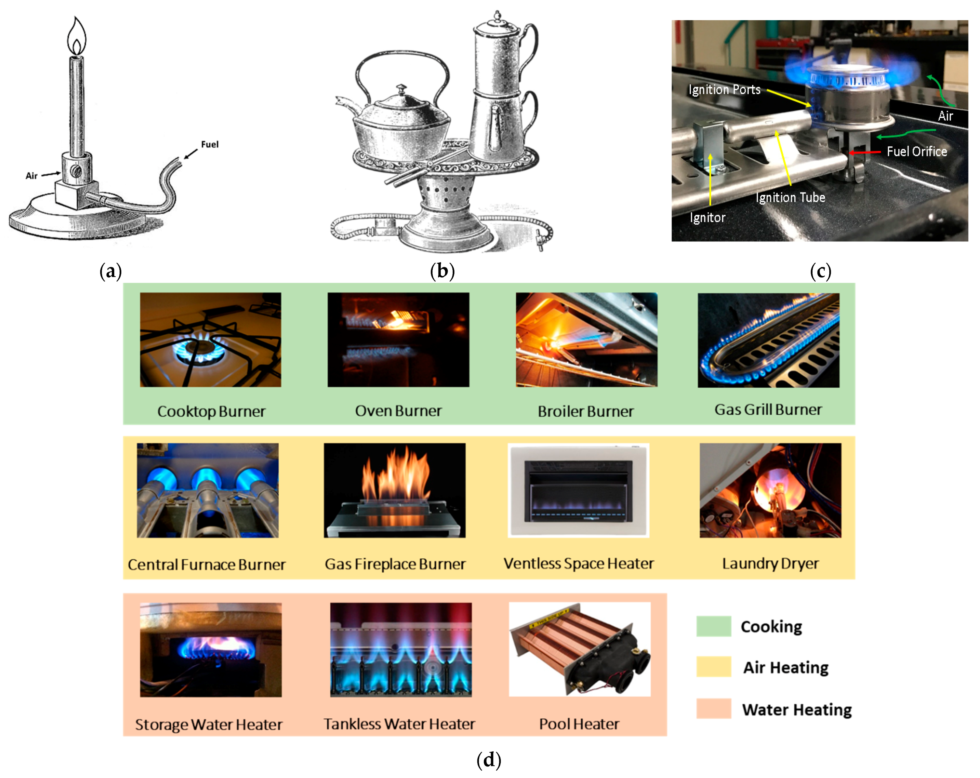
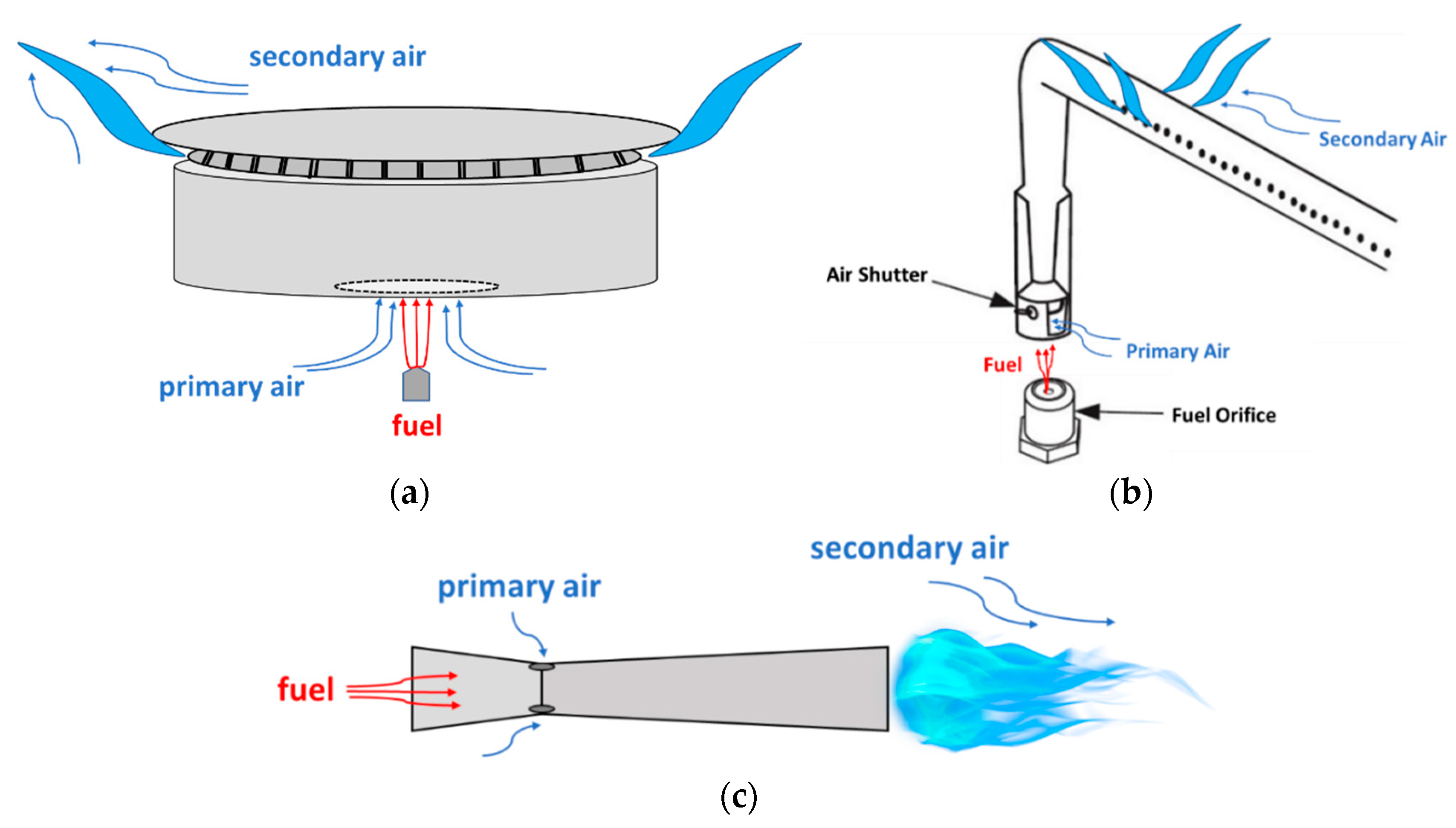
4.1. Working Principles of Residential Burners

Residential burners are usually mounted in domestic appliances. Compared to higher heating load gas burners designed for turbines or industrial applications, residential burners usually adopt simple designs that are easily manufactured, maintained, or replaced if damaged. Lacking complicated fuel/air flow control systems, most residential burners adopt self-adjusting fuel/air mixing technologies. The most common, if not the only, burner type in residential appliances is self-aspirating, also called an aspirated burner, whose flame type is usually partially premixed. This combustion technology was first introduced in the 1850s by the German chemist Robert Wilhelm Bunsen, who invented the later Bunsen burner and influenced the combustion applications and the gas industry significantly [52].

Figure 13a shows a model of the Bunsen burner. It is an atmospheric burner with a jet from a gas-aspirating part, and the air can be entrained through adjustable shutters into a fuel/air mixing tube before reaching the burner port for combustion. Due to the pre-mixing of fuel and air before combustion, the soot formation and carbon monoxide emissions are significantly diminished, and the flame length or position is more controllable by adjusting the air shutter. Therefore, the Bunsen burner gained popularity not soon after it was introduced to the public and was modified into various applications. Figure 13b shows a domestic aspirating burner for cooking and water heating in the late 19th century. As shown, the fuel is supplied to the burner through a valve at the bottom and then entrains some air through the small circular openings on the burner surface before reaching the flame zone. Till today, self-aspirating burners are still dominant in residential appliances. Figure 13c shows a representative cooktop burner that is available on the market today. As shown, fuel is injected into the burner head while entraining a small amount of surrounding air. Part of the mixture flows out of the ignition ports and arrives at the ignitor through the ignition tube. After ignition, the flame propagates to the burner head, and a full flame is established. Figure 13d shows that most of the current representative appliances on the market, including cooking, air-heating, and water-heating applications, use self-aspirating technology. As can be seen, most of the flames appear blue in color due to their relatively low equivalence ratio at operating conditions, which helps reduce soot, unburned hydrocarbons, and carbon monoxide emissions. However, due to different heating purposes, some appliances might glow yellow/red in color. For example, outdoor grillers usually have yellow tips to enhance heat transfer in grilling. A gas fireplace’s flame appearance is close to a diffusion flame because it needs the soot radiation to heat the surrounding space.

Due to the simple burner design and outstanding combustion performance, self-aspirating combustion is not only the most common combustion technique in residential homes but also in laboratories and the light industry.

Although these residential burners adopt the same combustion technology, their appearances might still be distinct from each other. Figure 14 shows the most common self-aspirating burner types in residential burners. Figure 14a shows the configuration of a flat self-aspirating burner, which usually has the fuel and primary air inlet at the burner bottom and flame at the top. The primary air is usually not adjustable for this simple design, and it is hard to replace the designated fuel with alternative fuels. This burner type is widely adopted in cookstoves and storage water heaters. Figure 14b is a tube burner, which is usually equipped with an air shutter at the fuel-injection location. This burner is used in ovens, broilers, outdoor grillers, etc. Figure 14c is a Venturi jet burner, which has the primary air suction openings at the smallest diameter of the burner. The Venturi effect produces a low pressure at the primary air opening area, thus helping aspirate more primary air into the burner. This burner type is usually used for higher-heating-load residential appliances, such as laundry dryers and room furnaces.

4.2. Fuel Properties

As discussed in the earlier chapters, the most used fuel in residential pipelines is natural gas, whose major content is methane. In the manufactured gas era, the major contents were carbon monoxide, hydrogen, and some higher hydrocarbons. Due to the toxicity of carbon monoxide, it is considered to be a dangerous substance in the residential pipeline and has already been eliminated in most residential pipeline systems around the world. However, due to its carbon-free property and ease of production from renewable energy sources, hydrogen might play an important role in future residential pipeline systems. Therefore,

Table 12. Property comparison among common residential fuels (at 298.15 K and 1 atm).

Fuel Properties	Unit	Propane (C3H8)	Ethane (C2H6)	Methane (CH4)	Carbon Monoxide (CO)	Hydrogen (H2)
Density	kg/m3	1.808	1.219	0.648	1.131	0.0813
Viscosity	10−5 Pa·s	0.82	0.94	1.11	1.8	0.89
Laminar Flame Speed (ϕ =1)	m/s	0.46	0.45	0.43	0.17 [160]	2.1
Low Flammability	ϕ	0.51	0.50	0.46	0.34	0.1 *
	vol%	2	3	5	12.5	4
High Flammability	ϕ	2.83	2.72	1.64	6.76	7.2 *
	vol%	11	14	15	74	75
Ignition Energy (ϕ =1)	10−5 J	30.5	42	33	-	2
Quenching Distance (ϕ =1)	mm	2.0	2.3	2.5	-	0.64
Adiabatic Flame Temperature (ϕ =1)	K	2267	2259	2226	2400	2318
Lower Heating Value	MJ/m3	83.9	57.9	32.4	11.5	9.8
	MJ/kg	46.4	47.5	50.0	10.2	120.1
Higher Heating Value	MJ/m3	91.1	63.3	36.0	11.5	11.6
	MJ/kg	50.4	51.9	55.5	10.2	142.1
Wobbe Index	MJ/m3	73.7	62.4	48.6	11.8	44.3

* It should be noted that the flammability range in [158] has errors. The correction is made through personal communication with Prof. Stephen Turns, and a corrigendum has been published under [117].

lists the key physical and chemical properties of representative residential gaseous fuels. The major fuel properties are from [158,159], with exceptions noted.

Lower hydrocarbons have smaller sizes of molecules, which result in a lower density and ease of leakage. Currently, the leakage of natural gas into the atmosphere from residential buildings is becoming a concern for climate change [161]. Additionally, if pipeline gas contains carbon monoxide, the leakage of this gas can be detrimental due to the density similarity between carbon monoxide and the air, which makes it harder for it to dissipate out of residential houses. Hydrogen has the smallest molecule and thus the lowest density among all the combustible fuels; therefore, hydrogen can more easily leak from pipelines. However, some studies also show that the leakage rate of hydrogen is at the same level as natural gas in low-pressure infrastructures such as a pipeline in residential buildings [162]. Due to the high reactivity of hydrogen, the leakage danger can be a big challenge in its residential applications. Some researchers are also arguing that the leakage of hydrogen might be less dangerous compared to other fuels because the low density of hydrogen increases its ventilation rate. Both numerical and experimental studies were conducted to evaluate the danger level of hydrogen leakage in residential houses, and results show that the ventilation rate of leaked hydrogen is highly dependent on the leakage rate and location [163,164]. There is no definite conclusion yet regarding the danger level of natural gas and hydrogen leakage.

Another important fuel property is the flame speed of the fuel. Table 12 compares the laminar flame speed of different fuels at stoichiometric conditions. As shown, listed hydrocarbons have a very similar flame speed, which is between 0.4 and 0.5 m/s. It is important to note that the laminar flame speed of hydrogen is around five times that of methane. This might increase the danger level of flashback when replacing the pipeline’s natural gas with hydrogen.

Another property difference is the fuel flammability range in air. Methane, which is the major content in natural gas, has a relatively small range of 5–15%. This property makes it a “safe” gas to be used in residential buildings. Ethane and propane have similar flammability properties. However, carbon monoxide and hydrogen have much wider flammable ranges, especially hydrogen. Hydrogen can be ignited when its volume percentage in the air is between 4% and 75%. This property brings extra challenges to fuel/air flow rate control and burner design.

The high reactivity of hydrogen is also reflected in its low ignition energy and smaller quenching distance. However, these properties also have positive influences on combustion performance. For example, the ease of hydrogen ignition can reduce the ignition time, which decreases the fuel leakage in the ignition process. Moreover, the high reactivity can also increase the flame stability to allow combustion to take place at a fuel-lean condition, which helps decrease thermal NO_X emissions by deviating the reaction from the stoichiometric condition. On the other hand, the adiabatic flame temperature of hydrogen is slightly higher than that of methane (around 4% higher in stoichiometric conditions). Therefore, in stoichiometric conditions, if the heat-release rate is kept constant, the theoretical thermal NO_X of hydrogen flames is slightly higher than that of methane.

An important fuel property for combustion is the heat-release rate, which is closely related to the heating value and the Wobbe Index. The heating value is either interpreted on a volume base or on a mass base. A higher heating value is usually used to describe the total heat release from the fuel, including the latent heat from the water in the exhaust. In contrast, a lower heating value does not consider the latent heat. It should be noted that natural gas is usually sold from utilities to customers with a higher heating value; however, most residential appliances cannot recover the latent heat. This means that we pay the gas bill for the higher heating value of the fuel, but we only use the lower heating value of the gas. It is important to note that some modern high-efficiency appliances, when equipped with water-condensing heat exchangers, can recover the latent heat from the exhaust. These appliances are usually of higher heating loads, such as room furnaces or water heaters. Appliances with water-condensing systems are usually labeled as having an energy efficiency higher than 90%.

As shown in

Table 13. AGA flame code classifications.

Code	Flame Description
+5	Flames lifting from ports with no flame on 25% or more of the ports.
+4	Flames tend to lift from ports but become stable after short period of operation.
+3	Short inner cone; flames may be noisy.
+2	Inner cones distinct and pointed.
+1	Inner cones and tips distinct.
0	Inner cones rounded; soft tips.
−1	Inner cones visible; very soft tips.
−2	Faint inner cones.
−3	Inner cones broken at top; lazy wavering flames
−4	Slight yellow streaming in the outer mantles or yellow fringes on tops of inner cones. Flames deposit no soot on impingement.
−5	Distinct yellow in outer mantles or large volumes of luminous yellow tips on inner cones. Flames deposit soot on impingement.

, the volumetric heating value of a gaseous fuel decreases as the fuel reaches lower hydrocarbons or carbon/hydrogen-free. However, on a mass base, the heating values of hydrocarbon fuels are at a similar level. Although the volumetric lower heating value of hydrogen is at 9.8 MJ/m³, which is around 30% of methane, the heating value of hydrogen on the mass base is more than twice that of natural gas. The Wobbe Index is usually correlated to the heat-release rate in combustion applications. It should be noted that although methane and hydrogen have distinct heating values, their Wobbe Index values are very similar, which is a positive sign for fuel interchangeability.

4.3. Interchangeability Considerations

Although all of the fuel properties can influence the combustion performance, there are some essential parameters that need to be considered ahead of other ones when it comes to fuel interchangeability. For example, the heating value and the Wobbe Index are two priorities regarding the heat-release properties of the fuels.

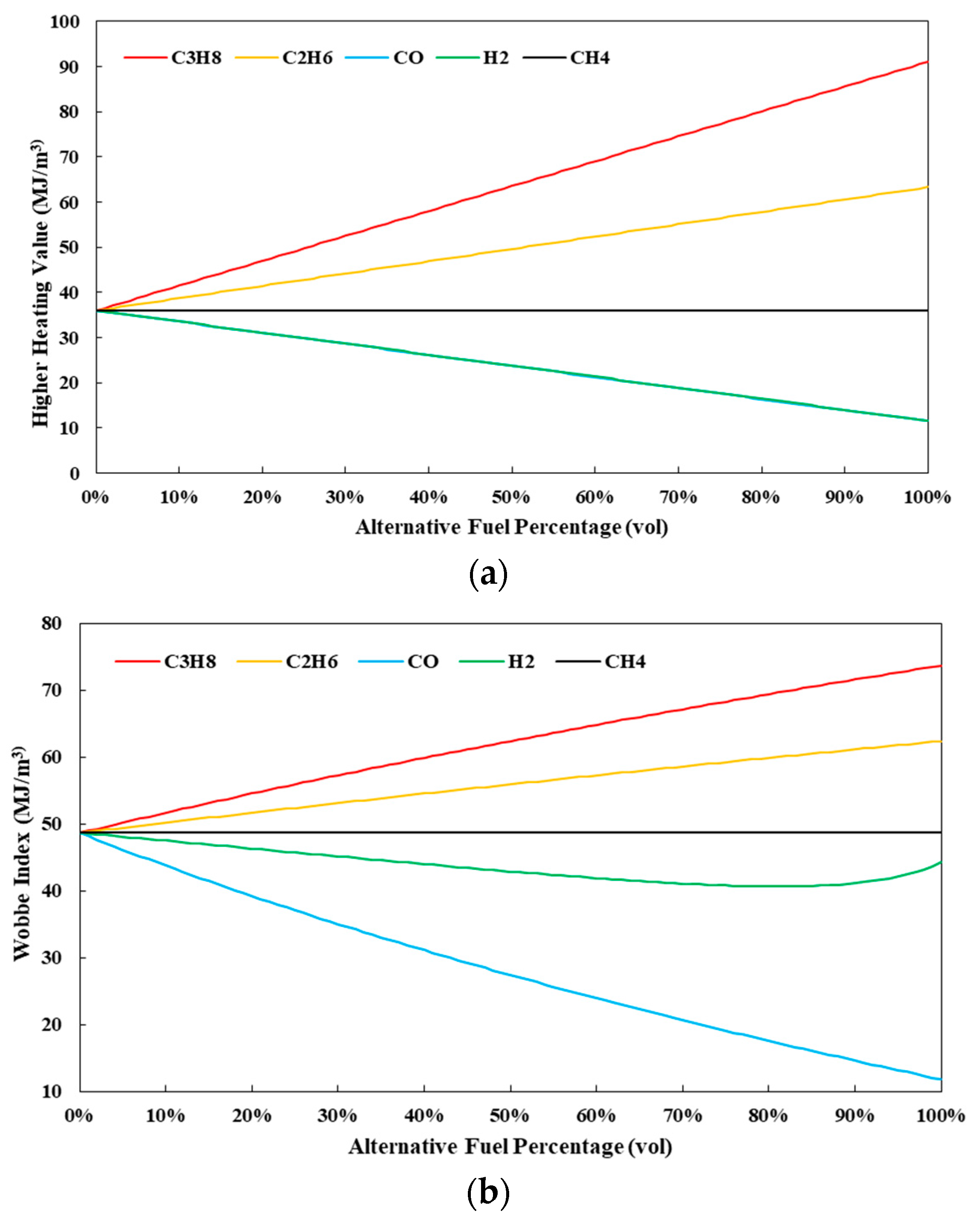
4.3.1. Heating Value and Wobbe Index

The major function of fuel is to convert its chemical energy into heat—this potential is presented as the heating value. Due to the similarity between natural gas and methane properties, methane is used to conduct analysis. The higher heating value and Wobbe Index of methane and other fuel mixtures are plotted in Figure 15.

Figure 15a shows the heating value curves of methane and other fuel mixtures. The volumetric heating value of methane is 36.0 MJ/m³ (298 K, 1 atm). With alternative fuels mixed with methane, the higher heating value of fuel mixtures shows a linear change. When methane is mixed with fuels of a higher heating value, such as propane and ethane, the volumetric heating value shows an increasing trend. However, when methane is mixed with hydrogen and carbon monoxide, the heating value of the mixture shows a decreasing trend. Due to the similarity of the higher heating value between hydrogen and carbon monoxide, the two lines overlap.

Differing from the fuel mixture heating value plot, the Wobbe Index plot does not show a linear plot due to the definition of the Wobbe Index.

$$\mathrm{Wobbe} \mathrm{Index}=\frac{\mathrm{Higher} \mathrm{Heating} \mathrm{Value}}{\sqrt{\mathrm{Fuel} \mathrm{Specific} \mathrm{Gravity}}}$$

(1)

While the Wobbe Index is widely adopted today, the concept of using the heating value over the square root of fuel density as a fuel-interchangeability parameter originates from an American Gas Association (AGA) study in the 1920s, as mentioned in the previous discussion. In this study, a “C-index” of change in performance of appliances was established as a critical parameter, which is the predecessor of the widely used Wobbe Index today.

To illustrate why the Wobbe Index can be used to predict the interchangeability of the heat-release rate, the Bernoulli equation can be used as a starting point, and a few assumptions can be made that are applicable to typical operating conditions of appliances. By assuming the fuel flow is at a steady state and the flow is incompressible (constant fluid density) and inviscid, the Bernoulli equation is reduced to Equation (2).

$$p_1+\frac{1}{2}{\rho }_f{V}_1^2=p_2+\frac{1}{2}{\rho }_f{V}_2^2$$

(2)

In the above equation, p₁ is the natural gas pressure in a household pipeline, which is at a low level, around 2000 Pa. For most appliances, combustion usually takes place in open-air conditions; therefore, p₂ is the atmospheric pressure. Equation (2) can be rearranged to solve for the volumetric flow of the gas exiting the fuel port:

$${\dot{V}}_f=A_2\sqrt{\frac{2\mathsf{\Delta }p}{{\rho }_f\left(1-{\left(\frac{A_2}{A_1}\right)}^2\right)}}$$

(3)

As shown, the volume flow rate of the fuel is a function of the fuel density, fuel flow areas, and pressure drop from the household pipeline to the combustion device. However, due to the relatively small orifice area for the combustion device compared to the gas feed cross-section, (A₂/A₁)² can usually be ignored, which leads to Equation (4).

$${\dot{V}}_f=A_2\sqrt{\frac{2\mathsf{\Delta }p}{{\rho }_f}}$$

(4)

Therefore, the heat output of a combustion device can be presented as

$$\dot{q}={\dot{V}}_{f}HHV=\sqrt{\frac{2\mathsf{\Delta }p}{{\rho }_{air}}}\frac{HHV}{\sqrt{s{g}_f}}$$

(5)

Based on the assumption of constant density and neglecting the viscous effect, the heat output of the combustion device is only a function of the heating value over the square root of the fuel-specific density.

$$\mathrm{Wobbe} \mathrm{Index}=\frac{HHV}{\sqrt{s{g}_f}}~\dot{q}$$

(6)

The reason why the Wobbe Index is good at predicting the heat output of different combustion devices is due to the validity of the assumptions in practice. The Mach number of the gas flow in the household pipeline is much smaller than 0.3. Therefore, it can be assumed that the gas is incompressible in the pipeline. When the gas flows through the orifice of a combustion device, the gas pressure drop can accelerate the flow, which will result in friction loss. However, the gauge pressure in the pipeline is only at around 2000 Pa, which is less than 2% of the atmospheric pressure. Therefore, the pressure loss is not significant.

The Wobbe Index of methane and alternative fuel mixtures (assuming alternative fuel takes x% of the volume in the fuel mixture) are given by Equation (7).

$$W{I}_{Mix}=\frac{\left(1-x\%\right)HH{V}_{CH4}+x\%HH{V}_{Al}}{\sqrt{\frac{\left(1-x\%\right){\rho }_{CH4}+x\%{\rho }_{Al}}{{\rho }_{Air}}}}$$

(7)

As shown in Figure 15b, although the heating values of hydrogen and methane are significantly different, they have similar Wobbe Index values. This observation leads to the consideration that part of the pipeline natural gas can be replaced with hydrogen without influencing the heat output in current combustion devices. In other words, a 5 kW burner will retain a nearly 5 kW rating when operating on natural gas/hydrogen mixtures.

4.3.2. AGA Indices

Even though the heating value and Wobbe Index are essential indicators for fuel interchangeabilities, they cannot predict all the other combustion performances, such as flame characteristics, flashback limits, and emissions. For example, due to the nonlinear character of the Wobbe Index definition, a 37% hydrogen/63% methane mixture has the same Wobbe Index as pure hydrogen. These two different fuel classes might have the same heat-release rate in a combustion device; however, their combustion performances should differ from each other significantly. Therefore, there are also other flame indices that can help predict the combustion performances besides the heat-release rate, such as flame lifting, flash-back, and a yellow tip.

The most widely applied flame indices are AGA flame indices regarding flame lifting (I_L), flame flashback (I_F), and yellow tip (I_Y) [82,165,166]. It should be noted here that in [82], the flame-lifting index (I_L) was wrong.

$$I_L=\frac{K_a}{\frac{f_a{a}_s}{f_s{a}_a}\left\{K_s-\log \left(\frac{f_a}{f_s}\right)\right\}}$$

(8)

$$I_F=\frac{K_s{f}_s}{K_a{f}_a} \sqrt{\frac{H_s}{39934}}$$

(9)

$$I_Y=\frac{f_s{a}_a{Y}_a}{f_a{a}_s{Y}_s}$$

(10)

-

K: lifting limit constant; a: volume of air theoretically required for complete combustion; f: primary air factor; H: a higher heating value of the fuel (unit: kJ/N·m³); Y: yellow tip coefficient.

-

Subscripts a and s: designating adjustment and substitute gases, respectively.

AGA flame codes are listed in Table 13. When the code stays at low absolute values, the flame is predicted to be acceptable. Gas utility companies usually have their own AGA index regulations. For example, the SoCalGas Company in the U.S. has the following requirement: I_L ≤ 1.06, I_F ≤ 1.2, I_Y ≥ 0.8.

4.3.3. Weaver Indices

Another series of the interchangeability index is the Weaver index series [82]. This series included the considerations of all AGA indices and three other additional indices. The additional indices are the consideration of the Wobbe Index, primary air entrainment, and incomplete combustion prediction.

The heating load index (J_H) is the ratio of the substitute gas Wobbe Index over the original gas Wobbe Index. As J_H becomes close to 1, it becomes easier to keep the heating load constant while replacing the original fuel with the substitute gas.

$$J_H=\frac{H_s\sqrt{D_a}}{H_a\sqrt{D_s}}=\frac{W{I}_s}{W{I}_a}$$

(11)

-

D: specific density of the fuel

The primary air index (J_A) shows the change in the primary air that accompanies a change of gas. It is indicated by Weaver that this index not only provides an accurate measure of primary air to burn two gases but an almost accurate measure of secondary air as well. The ideal value of J_A is also 1.

$$J_A=\frac{a_s\sqrt{D_a}}{a_a\sqrt{D_s}}$$

(12)

-

a: volume of air theoretically required for complete combustion

The lifting index (J_L) notes the relative tendency for flames of the two gases to lift from the burner ports. When J_L = 1, the two gases are interchangeable regarding the flame position.

$$J_L=J_A\frac{S_s}{S_a}\frac{100-Q_s}{100-Q_a}$$

(13)

-

S: flame speed of the fuel in the air.

-

Q: percentage of oxygen in the gas.

The flashback index (J_F) shows the relative tendency for flames of the two gases to flash back into the burners. J_F = 0 indicates there is no difference between the gases in this respect.

$$J_F=\frac{S_s}{S_a}-1.4J_A+0.4$$

(14)

The yellow tip index (J_Y) indicates the tendency of fuel-producing soot, therefore yellow tips, in flames. As shown in the definition, the higher content of carbon in a fuel, the higher the index can be. Therefore, the ideal value for J_Y is 0.

$$J_Y=J_A+\frac{N_s-N_a}{110}-1$$

(15)

-

N: the number, in 100 molecules of gas, of the total carbon atoms minus one, except for methane.

The last index in this series is the incomplete combustion index, which is used to represent the tendency of a fuel to produce unburned hydrocarbons or carbon monoxide in the exhaust. When the two gases are equally likely to liberate carbon monoxide during combustion, J_I = 0.

$$J_I=J_A-0.366\frac{R_s}{R_a}-0.634$$

(16)

-

R: the ratio of hydrogen to carbon atoms contained in the fuel.

4.3.4. Other Indices

The AGA indices and Weaver indices are the two most widely applied flame index series regarding fuel interchangeability. Although the Weaver index series (six total) is more comprehensive in covering flame characteristics, the three AGA indices are more commonly adopted by gas utilities around the world. This is because gas utilities usually have their own regulations on fuel species, the heating value, and the Wobbe Index. These basic regulations from utility companies ensure that the combustion performance of the substitute fuel does not deviate from the original fuel too significantly. After the substitute fuel meets all requirements, the application of the AGA Index can help further test the flame lifting, flashback, and yellow tip performance.

Besides the AGA and Weaver indices, there are also other indices developed around the world to predict interchangeability among gaseous fuels. They are usually considered or adopted in scientific research because they are either too focused on one or two combustion performances or too complicated to be applied in industrial applications. The other indices are listed in

Table 14. Flame indices besides AGA and Weaver indices.

Name	Description	Reference
Knoy index	Similar to Wobbe Index, which predicts heat-release rate interchangeability.	[167]
Dutton indices	This series of indices mainly considers the incomplete combustion behavior or near blow-off condition for higher hydrocarbons. It consists of incomplete combustion index, lift index, and soot index.	[168]
Delbourg indices	This series is composed of two indices: yellow tip index and soot-formation index.	[168,169,170]

.

5. Residential Burner Performance Evaluation

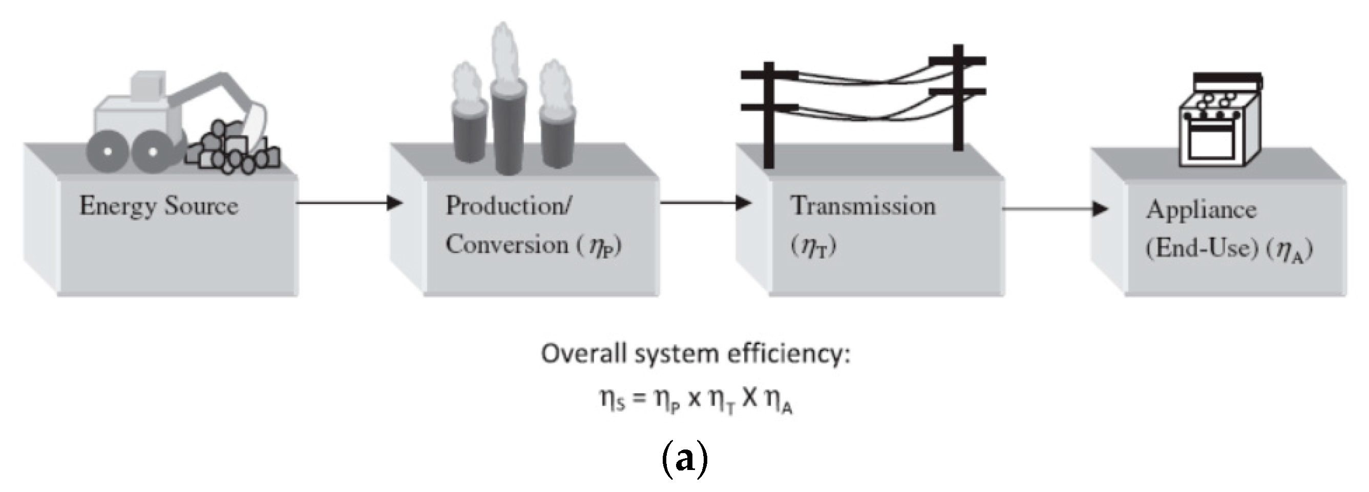
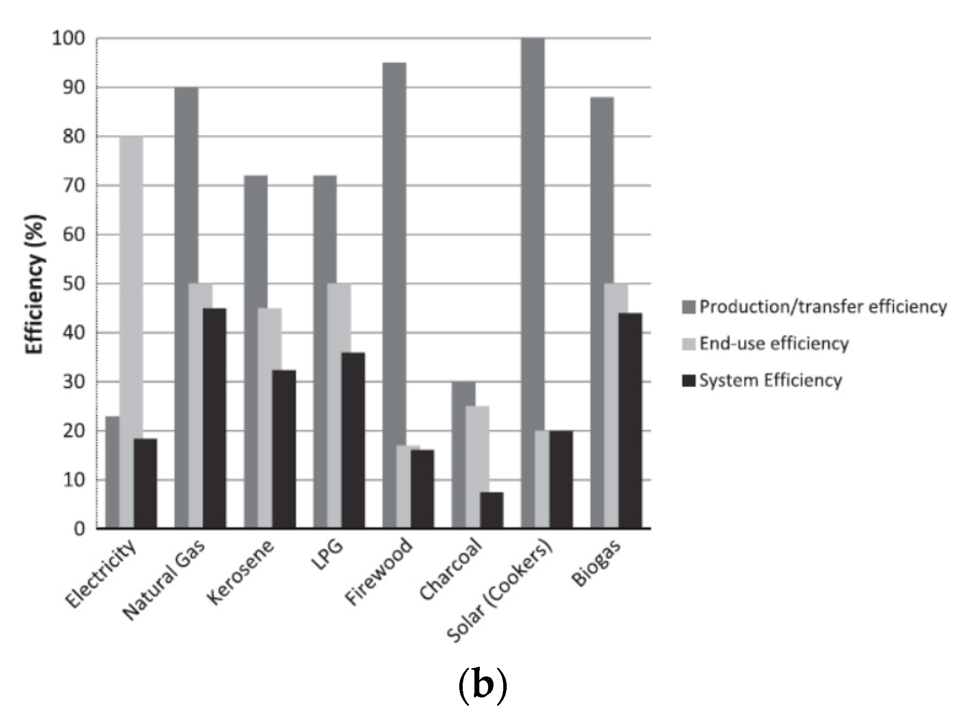
5.1. Efficiency

Efficiency, which is directly related to the utility bill, is one of the primary considerations for a residential householder choosing an appliance. Therefore, improving efficiency has always been a motive for appliance manufacturers to upgrade their products. To guide the residential sector to a higher energy-efficiency level, regulations are also being improved to promote this process worldwide [171]. Among all the energy-efficiency-promoting programs, the most influential one might be the ENERGY STAR program executed by the U.S. Environmental Protection Agency and the U.S. Department of Energy in 1992 [172]. Over the past few years, this program has been adopted worldwide, including in the European Union, Japan, and Australia.

For gas appliances, the efficiency of an appliance is closely related but not equal to the burner’s combustion efficiency. The combustion efficiency of a burner is the ratio of the total heat release over the total chemical energy in the fuel. Therefore, the major combustion efficiency loss is from the unburned hydrocarbons or carbon monoxide emissions. In modern residential appliances, these emissions are mostly at the ppm level, which makes the combustion efficiency close to 100%. Therefore, the appliance efficiency loss is most likely from aspects regarding the appliance’s inner structure design, including the burner location, heat-exchanger arrangement, etc.

It should also be noted that a high appliance efficiency can also be coupled with a low combustion efficiency, which might increase the emission levels. For example, in a cooktop burner support rack optimization process, it was found that the lower rack could shorten the distance between the flame and the cooking utensil, which helps reduce radiation loss to the environment, thus increasing efficiency. However, this also results in flame impingement onto the cooking utensil surface and can increase the carbon monoxide emission level and also degrade the cooking utensil’s lifespan [173]. Therefore, improving appliance efficiency is a task that involves numerous aspects; sometimes, a compromised efficiency level should be adopted to optimize other aspects of the appliance’s performance.

Among various residential appliances, water heating and air heating efficiency are relatively easy to measure using the energy output/input method. Most of the existing room furnaces can easily achieve an energy efficiency of 80%, and water heater efficiency can be higher than 90% with a latent-heat-recovering (water-condensing) system [120,122].

Compared to the mature efficiency testing method for air/water-heating appliances, there is yet to be a universal efficiency testing standard for cooking appliances. In contrast to air/water heating, heating food to a certain temperature is not the only purpose of cooking, so it is relatively hard to define a perfect cooking process. However, efforts are still being made around the world to quantify cooking efficiency to help improve cooking appliances’ performance. As shown in

Table 15. Cooking appliance efficiency evaluation methods.

Name	Method	Reference
Food cooking	Cooking a specific food (egg, etc.) and evaluating the food appearance to interpret efficiency	[174,175]
Water boiling	Boiling water and calculating the ratio of heat absorbed by water over the total heat-release rate	[116,117,176,177,178,179,180]
Object heating	Heating some materials (usually metal rod/disk) and measure the temperature change of the material to quantify the efficiency	[181,182]

, the most common ways to evaluate cooking efficiency are food cooking, water boiling, and object heating. Cooking a specific food is an intuitive way to evaluate cooking performance. For example, Oberascher [174] used boiling eggs and cooking potatoes to evaluate the cooking performance of different cooking appliances. To evaluate the cooking results, the egg yolk status was scaled to five levels: very liquid, liquid, a firm outer edge, can be separated from the egg white, firm, and dry. The egg yolk status was also coupled with the yolk color judgment to distinguish the cooking efficiency of different appliances. Cheng [175] conducted experiments on meat and used the meat moisture loss rate as one of the cooking efficiency measurement methods. The food cooking method is effective in evaluating the cooking performance at one location and time, but it is relatively hard to repeat the results for other testing locations or even the same location at different times due to the tested food quality variation. Moreover, it is also hard to generate a universal quantified standard to evaluate the cooked food characteristics related to cooking efficiency.

Therefore, the water boiling test is more widely adopted to evaluate cooking appliances’ efficiency. To avoid the influence of cooking utensils on cooking efficiency, the American National Standards Institute (ANSI) regulated the dimension of the water boiling pot and testing method [176]. Although boiling water deviates from the actual cooking process, it is relatively easy to quantify the cooking efficiency using Equation (17). Efficiency is defined as the heat absorbed by water (including the latent heat from the escaped water vapor) over the total heat released from the fuel. Most cooking appliances cannot recover heat from the water vapor in the exhaust; therefore, a lower heating value is usually adopted to calculate the heat released from the fuel.

$${\eta }_{cooking}=\frac{c_{p, water}*m_{water}*\mathsf{\Delta }T+h_{vapor}*\mathsf{\Delta }{m}_{vapor}}{V_{fuel}*LHV}$$

(17)

Heating an intermediate object instead of food or water is also a method to evaluate the cooking efficiency by measuring the object’s temperature variance over time. The material should be able to resist high temperatures and have high thermal conductivity; therefore, metals such as steel or aluminum are usually adopted [181,182]. This method requires the temperature of the intermediate object being relatively uniform over time, so it is more commonly adopted in oven testing.

It should be emphasized that the cooking speed and cooking efficiency are different from each other when evaluating the cooking performance of different fuel classes. If the heat-release rate is constant for two testing conditions, a faster cooking time can be regarded as higher efficiency. However, when the fuel classes have different heating values or Wobbe Index values, less cooking time can also result from a higher heating load of the burner. In this case, faster cooking, which might result in overcooking, may become a non-ideal situation. For example, Zhao et al. [116] evaluated the cooking efficiency of a cooktop burner operating on natural gas and biogas. The results showed that the cooking time increased as natural gas was replaced by biogas due to the heating load decreasing. However, the cooking efficiency stayed at a constant level. The cooking performance of a cooktop burner operating on natural gas/hydrogen mixtures was also tested. It was found that both the cooking time and efficiency did not change much up to 50 vol% hydrogen added into natural gas [117].

5.2. Emissions

Besides increasing efficiency, reducing emissions from appliances is also one of the major incentives for appliance manufacturers due to the stricter emission regulation worldwide. In the past few decades, combustion technologies have been advanced to reduce emissions, mainly in power generation, transportation, and industry. However, the emissions from the residential sector did not draw as much attention as other energy-utilization sectors. Residential appliances are closely related to our daily life, so the emissions from them not only harm the environment but might also threaten our health. Therefore, the existing emission regulations on appliances and the current emission levels of existing appliances should be understood as projecting the future.

5.2.1. Residential Appliance Emission Regulations

Currently, the emission regulations on power generation, transportation, and industrial applications are frequently updated and widely adopted worldwide. These regulations also play a significant role in motivating combustion technology advancement in power generation. It is believed that strict emission regulations for residential appliances can also stipulate the development of residential combustion technologies.

One of the most active agencies promoting appliances standards is the American National Standard Institute (ANSI) and the Canadian Standards Association (CSA). They update the ANSI-CSA standards on appliance performance every few years. Currently, the ANSI-CSA standards are not only adopted in North America but are also being learned and adopted by more countries worldwide. However, the ANSI-CAS standards only cover carbon monoxide emissions for safety reasons while lacking regulation on other emissions, such as nitrogen oxides. Therefore, the ANSI-CSA standards have to be coupled with other standards to form a more comprehensive emission-regulation series, especially standards regulating nitrogen oxides emissions. One of the most pro-active regions regulating NO_X emissions and promoting new combustion–pollutants control technologies is California (U.S.). To deal with the Los Angeles smog hazard caused by NO_X-O₃ photochemical reactions, several environmental-protection and emission-regulation-promoting agencies were founded after the U.S. Congress passed the Clean Air Act in 1963. These agencies include the U.S. Environmental Protection Agency (EPA, 1970) promoting federal regulations, the California Air Resources Board (CARB, 1967) regulating vehicle emissions, and the South Coast Air Quality Management District (SCAQMD, 1976) issuing emission standards on standard sources of air pollution. Among these agencies, the SCAQMD issues emission regulations for multiple sectors, including industrial and residential applications.

Table 16. Representative emission regulations for residential appliances in North America.

	Regulation Title	Agency	Adopted Time	Major Contents
Water-heating appliances	ANSI Z21.10.1 [183] ANSI Z21.10.3 [184]	ANSI-CSA	2017	CO < 800 ppm (heating load ≤ 75,000 Btu/h). CO < 400 ppm (heating load > 75,000 Btu/h).
	Rule 69.5.1 [185]	SDCAPCD	2017	NOX < 10 ng/J (calculated as NO2) or NOX < 15 ppm (@ 3% O2, dry).
	Rule 1121 [186]	SCAQMD	2004	NOX < 10 ng/J (calculated as NO2) or NOX < 15 ppm (@ 3% O2, dry).
Space-heating appliances	HSC-1988 [187]	California Law	1997	No person shall sell, or offer for sale, any new or used unvented heater that is designed to be used inside any dwelling house or unit, with the exception of an electric heater or decorative gas logs for use in a vented fireplace.
	ANSI Z21.86 [188]	ANSI-CSA	2016	CO: less than 200 ppm in the air free sample.
	Rule 4905 [189]	SJVAPCD	2018	NOX: 14 ng of oxides of nitrogen (calculated as NO2) per joule of useful heat delivered to the heated space.
	Rule 1111 [190]	SCAQMD	2018	NOX: 14 ng of oxides of nitrogen (calculated as NO2) per joule of useful heat delivered to the heated space.
Cooking appliances	Rule 1153 [191]	SCAQMD	1995	VOC of commercial bakery ovens (≥2 million Btu/h) should be less than 50 pounds/day.
	Rule 1138 [192]	SCAQMD	1997	Chain-driven charbroiler must be equipped with catalytic oxidizer reducing PM and VOC.
	Rule 1131 [193]	SCAQMD	2003	The VOC content of each solvent used ≤120 g per liter of material.
	Rule 1153.1 [194]	SCAQMD	2014	Commercial ovens: CO: 800 ppm (@ 3% O2). NOX: 40 ppm (@ 3% O2)-500 °F-60 ppm (@ 3% O2).
	ANSI Z21.1 [176]	ANSI-CSA	2016	CO: cooking appliances less than 800 ppm.
	Rule 4692 [195]	SJVUAPCD	2018	In lieu of SCAQMD-Rule 1138. The catalytic oxidizer shall have a control efficiency ≥ 83% for PM-10 emissions and a control efficiency ≥ 86% for VOC emissions.

lists the existing emission regulations for residential appliances in North America, which is also considered as one of the strictest regulation series in the world. It should be noted that most of these regulations are only adopted in very few places around the world. For example, some of the NO_X emission regulations from SCAQMD are not even extensively adopted in California itself. However, these regulations should indicate the future of appliance emissions levels worldwide.

For residential water-heating appliances, the ANSI-CSA regulates that CO should be lower than 400 ppm or 800 ppm in an undiluted exhaust sample for water-heating appliances of different heating loads [183,184]. The most widely adopted NO_X standard in the U.S. is the SCAQMD-14 ng/J emission regulation [186]. The water heaters that adopt this regulation are usually labeled low-NO_X water heaters on the market. The ultra-low-NO_X 10 ng/J standard is from the San Diego County Air Pollution Control District (SDCAPCD) [185], which is being adopted by more and more residential water-heater manufacturers.

Space heating is also a major emission contributor from residential houses. In 1997, California banned the sale of ventless space heaters in residential homes. Currently, vented heaters being sold or installed in California, the CO emission should be lower than 200 ppm [188]. Additionally, the maximum NO_X emission of residential water heaters dropped from 40 ng/J to 14 ng/J. If the residential water heaters on the market cannot meet this standard by the year 2021, a penalty will be paid by manufacturers for each water heater unit sold in California [122,189,190].

Currently, the major emission regulations on cooking appliances are mainly for VOC or particle emissions from the food, which requires ventilation in the kitchen. The threatening emissions to human health from kitchens are mainly particle emissions instead of emissions from kitchen flames [196,197]. However, residential houses with bad ventilation might have CO and NO_X accumulation in the living space, which creates health issues. Even if the direct influence of residential flame emissions on human health is negligible compared to particle emission from food itself, reducing kitchen flame emissions should also help reduce the total emissions released into the atmosphere. Due to the uncertainness of kitchen burners’ operating conditions, ANSI-CSA imposes a relatively “generous” restriction on CO emission (400 ppm/800 ppm) compared to water and space heaters. Although there are no direct NO_X emission regulations on residential cooking appliances, SCAQMD restricts the NO_X emission of commercial ovens to lower than 40 ppm at an operating temperature lower than 500 °F. With the oven temperature exceeding 500 °F, the NO_X emission limit is extended to 60 ppm.

It should be noted that the emission regulations in Table 16 are mainly for gaseous fuels. There are still a lot of developing countries and even some areas in developed countries that use wood, coal, or biomass as residential heating/cooking energy sources. For these areas, particle emissions might be a larger or more direct threat to human health.

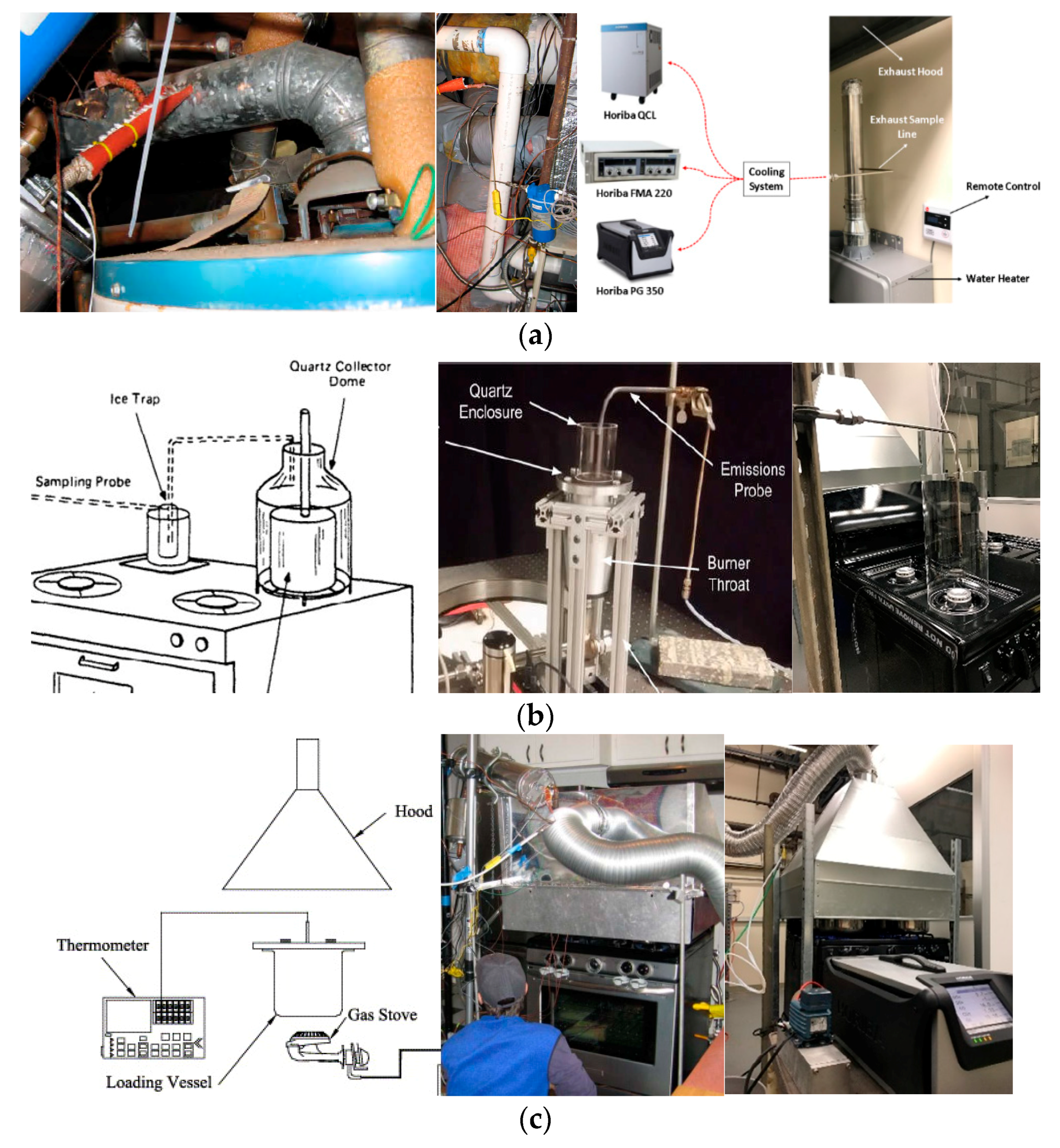
5.2.2. Emission Evaluation Methods’ Conclusion

As can be seen in Table 16, there are multiple ways to interpret emission levels of an appliance: for instance, the volume percentage in an undiluted exhaust sample (ppm), volume percentage at a corrected oxygen concentration (ppm @ 3% O₂), and emission level per unit energy output (ng/J). The lack of universal standards is reflected in the different ways to interpret emission levels. In fact, not only the emission level interpretations of residential appliances are hard to achieve a consensus on, but there are also various sorts of emission-testing methods.

As shown in Figure 16a, secured exhaust sampling is an ideal way to sample the emissions from an appliance’s exhaust-venting location. This is an effective method to avoid air dilution in the exhaust. However, this method is only practical for confined combustion appliances such as room furnaces or water heaters. Before all the exhaust is vented into the atmosphere, it will first be directed into a pipe, which the sampling probe can be located at.

However, a large number of residential burners have open-air flames, which means combustion takes place in an open space and dilution from the surrounding air is inevitable. Therefore, quartz enclosure and hood sampling methods are usually adopted, as shown in Figure 16b,c, respectively. The quartz enclosure sampling method is more suitable for small-sized burners. When adopting this method, it is necessary to make sure that the sampled mixture is homogeneous. If not, multiple locations within the quartz enclosure should be tested over a certain time period, and the average should be calculated to present the emission level of a burner. The exhaust hood sampling method is more commonly adopted for kitchen burners. The exhaust hood collects all the emissions before venting them into the atmosphere. Before the sample is taken from the hood, the exhaust mixture should be homogeneous. The distance between the hood and the burner should be especially emphasized. The hood should be close enough to the burner so that all the exhaust can be collected; otherwise, the tested emission level will be lower than the actual level. However, if the hood is too close to the flame, it might cut off the source of the oxidants (air) to the flame, which results in a carbon monoxide increase in the exhaust. ANSI Z21.1 recommends this gap should be around 5 inches (12.7 cm).

As shown above, the emission tests on residential burners are sometimes naturally diluted. Even for confined combustion, such as water heaters and room furnace burners, the secondary air from atmosphere also dilutes the emission to a lower absolute level. Therefore, the emissions are usually corrected under a certain reference level so they can be compared with each other.

A common emission correction method is to covert the absolute value of the emission to a certain oxygen level in the exhaust. As shown in Equation (18), the emission is corrected at 3% O₂.

$${\left[X\right]}_{3{\% \mathrm{O}}_2, \mathrm{ppm}}={\left[X\right]}_{\mathrm{abs}, \mathrm{ppm}}\frac{20.9-3}{20.9-{\left[{\mathrm{O}}_2\right]}_{\mathrm{abs},\%}}$$

(18)

The oxygen correction method has already been verified to be valid in industry, and so it is applied to the residential sector. Zhao et al. [119] compared the influence of the air dilution on an oven’s emission and found that the oxygen correction method could interpret the emission level without bias. As shown in Figure 17a,b, two exhaust methods were adopted and compared with each other: flue collar sampling without dilution and hood sampling with significant dilution. As shown in Figure 17c, the emissions have periodic readings due to the oven burner’s automatic on/off switching to keep the temperature constant. As can be seen in the figure, by the end of the first period, the flue collar sampling method has a NO reading of 35 ppm with 15% O₂ in the exhaust. When the exhaust hood is adopted, the NO emission level is diluted down to around 10 ppm with 19% O₂ in the exhaust. However, when the emissions readings of these two methods are both corrected to 3% O₂, they show a very similar emission reading in spite of the significant difference in dilution.

Another common reference level is 12% CO₂. This is because the carbon dioxide percentage in the dry exhaust for natural gas oxidized in the air in stoichiometric conditions is close to 12% [202]. This correction method is sometimes called the “air-free” method. The 12% CO₂ correction is shown in Equation (19). However, it should be noted that this correction method might increase the corrected emission level when carbon-free fuel (such as H₂) is added to the original fuel. This is due to the intrinsic property of Equation (19): the CO₂ percentage of the exhaust is in the denominator, which decreases as the carbon-free fuel percentage increases. For example, Zhao et al. [122] tested a room furnace burner operating on natural gas/hydrogen mixtures with the hydrogen percentage increasing from 0 to 40%. Although the 3% O₂ correction method shows a flat emission curve, the 12% CO₂ gives an obvious increasing trend for all emissions.

$${\left[X\right]}_{12{\% \mathrm{CO}}_2, \mathrm{ppm}}={\left[X\right]}_{\mathrm{abs}, \mathrm{ppm}}\frac{12}{{\left[{\mathrm{CO}}_2\right]}_{\mathrm{abs},\%}-{\left[{\mathrm{CO}}_2\right]}_{\mathrm{air},\%}}$$

(19)

Equation (20) presents the calorific correction, which is also considered as a reliable emission correction method due to its independence from the exhaust species. In theory, the representation provided by calorific correction should be the most robust because it is independent of both O₂ and CO₂ in the clarification. However, it requires more information to be known in addition to the adjusted measured emissions levels, which makes it inherently more difficult to implement.

$${\left[X\right]}_{\mathrm{ng}/\mathrm{J}}=\frac{0.1·{\left[X\right]}_{\mathrm{abs}, \mathrm{ppm}}}{{\left[{\mathrm{CO}}_2\right]}_{\mathrm{abs},\%}-{\left[{\mathrm{CO}}_2\right]}_{\mathrm{air},\%}}\frac{{\mathrm{mol} \mathrm{CO}}_2}{\mathrm{MJ} \mathrm{Fuel}}{\mathrm{M}}_{\mathrm{X}, \mathrm{g}/\mathrm{mol}}$$

(20)

5.3. Flame Characteristics

As shown in Table 13, most flames of residential appliances should have a relatively small absolute code value. The flame cones are usually blue in color and have laminar flame characteristics. However, there are also exceptions. Since stable laminar flames are more likely to have a low flow rate, they are more for lower-heating-load appliances. Higher-heating-load appliances, such as room furnaces and laundry dryers, tend to have turbulent flames. Moreover, not all flames are supposed to have blue color. Gas fireplaces need to generate soot to promote radiation; therefore, the flames are usually yellowish or orangish. Although the yellow tip index was developed to guide fuel selection, avoiding yellow tips, outdoor grillers are allowed to have yellow tips, which help increase the heat-transfer rate to the food.

When replacing natural gas with renewable gases, the flame characteristics should be re-evaluated. For example, a hydrogen flame is invisible under sunlight, which might limit its use in existing gas fireplaces or outdoor grillers. The light flame color of hydrogen-rich fuel might also cause danger if an existing flame cannot be identified. However, researchers around the world also find a random reddish glow in hydrogen flames. It is believed that the color is from a contaminant in hydrogen, which might be related to the hydrogen embrittlement effect on metals [118].

5.4. Ignition Performance

Appliance ignition is also a crucial aspect of evaluating the performance of an appliance. Failure of ignition can result in natural gas leakage into residential homes, which endangers the safety of residents. Moreover, a long ignition time also results in methane leakage into the atmosphere for natural gas appliances. The greenhouse gas effect of methane is about 20 times that of carbon dioxide; therefore, the methane emissions from a delayed ignition also contribute to the greenhouse effect [161,203]. Some regulations set an upper limit for appliance ignition time. For example, ANSI Z21.1 [176] requires that residential cooking appliances achieve ignition within four seconds. Higher-heating-load appliances need an even stricter ignition time limit. ANSI Z21.86 [188] regulates that room furnace ignition should be completed within 0.8 s.

Ignition is an unsteady process, which might become a limiting factor for fuel-interchangeability studies. For example, Zhao et al. [117,204,205] replaced more than 75% of natural gas with hydrogen without having flashback in a cooktop burner under steady operating conditions. However, ignition flashback only occurs at 20% hydrogen addition. This is because, in steady operating conditions, the mixture within the burner is usually fuel-rich and out of the flammability range. In ignition conditions, when the fuel starts to fill the burner, the existing air within the burner makes the mixture fall into the flammability range. This causes ignition flashback.

Therefore, ignition performance should draw special attention to the burner design or residential appliance regulations.

5.5. Other Aspects

Other performance metrics are also considered in residential appliance evaluations, such as the burner temperature and combustion noise [117,119,122,206,207]. Modern appliances not only require high durability and working performance, but they are also expected to occupy a small space and have a neat design or even esthetic appearance.

6. Conclusions and Future Prospects

This paper summarizes the historical development of the residential fuel transition and appliances. Future energy transition and energy structure in the residential sector are projected. Following are the major conclusions and future prospects:

Almost every energy transition in human history was initiated in the residential sector. This residential energy source transition is either forced by the higher price of traditional fuels or a result of new needs. For example, the urbanization and industrialization in Europe first caused scarcity of fuelwood and forced the residential sector to turn to coal combustion. As coal needs developed in residential heating, mining technology was advanced, and coal’s transportation costs decreased. When the coal price became lower than fuelwood, the industry sector started to switch its energy source to coal, which boosted coal utilization worldwide. The oil industry was first initiated by residential lighting needs. Kerosene was extracted from crude oil to extend the lighting duration and quality. By that time, gasoline was just an abandoned by-product due to its high volatility, which made it difficult to store and use safely in the residential sector. However, as transportation needs increased, the cheap price of gasoline witnessed the booming of the transport engine industry. Natural gas was first regarded as a waste product in the oil industry and was usually vented into the atmosphere. This cheap or almost free gaseous fuel was first transported and utilized in nearby residential houses. Now, natural gas is one of the major fuel sources in the world. Thus, the residential sector fuel choice is interactive with large energy consumption sectors, such as industry and transportation, and on many occasions in history, it was the lead end use for exploring future fuel sources.

The power generation, transportation, and industrial sectors have received attention for centuries due to high energy consumption and demand and the adoption of novel technologies. This is in sharp contrast with the simple light and heating needed by the residential sector. This leaves sectors with a large energy consumption with time lag for energy transition due to their high demand for capital investment for equipment upgrades when facing an energy transition. In contrast, residential appliances are more focused on fuel itself and therefore are quicker to respond and to adapt during an energy transition. The inertia of power generation, transportation, and industrial applications transitioning to renewable energy systems inhibits steps that could be taken against climate change. The more flexible residential sector is, therefore, in the leading position again for transitioning into a renewable future.

The challenge of electrifying the residential sector by 100% is significant, perhaps not practical, based on the current power-generation technologies. Most of the residential needs, such as cooking, air heating, and water heating, come from a low grade of energy: heat. By electrifying the residential sector, the energy loss in electricity generation, transport, and conversion from electricity to heat is significant. Currently, more than 70% of the power in the world is still from combustion. Because the renewable energy sources are far from meeting the current energy needs in the world, electrifying the residential sector might increase the burden on power generation using combustion technologies and might result in more greenhouse gas emissions due to the efficiency loss in the electrification process.

The energy transition of the 21st century might be different from previous transitions. Most of the previous transitions were among existing fossil fuels, and the technology was mainly combustion. However, due to the scarcity and environmental impact of fossil fuels, future energy sources must involve various energy forms and a large number of new technologies. This energy transition in the residential sector will not only be led by the fuel market, but it also highly involves the policymaking by governments considering carbon emission reduction, air pollution control, and energy security issues.

Even if new energy sources are being invented in great numbers, it is very unlikely that the old energy sources will be completely abandoned. For example, even in developed countries, large numbers of people still use traditional energy sources such as burning crop residuals or coal. Renewable gaseous fuels such as biogas and renewable hydrogen are becoming strong competitors serving as an energy source for the future. These renewable gases can be generated by biomass or P2G technologies from solar, wind, hydropower, etc. Compared to the high capital investment and expensive operation and maintenance of fuel cells and solar panels for residential houses, replacing current pipelines’ natural gas with renewable gases can be an easier method for the residential energy transition. For a long period of time, maybe hundreds of years to come, combustion technology will coexist with other technologies. As pipelines’ natural gas can be replaced by renewable gases and renewable gases are energy carriers for different renewable technologies, combustion might be able to sustain its market share in residential applications, if not increase its share.

Incorporating renewable gases in residential houses requires a re-evaluation of the interchangeability criteria. Technical terms such as fuel mixture properties and flame indices need to be considered collectively. The flame indices being used by the residential sector are from the 1930s, by which time greenhouse gas emissions or air pollutants such as NO_X were not yet considered or understood at all. Therefore, for future fuel-interchangeability studies in residential appliances, new flame indices might need to be developed.

Compared to the frequently updated regulations on gas turbines, car engines, or industrial combustion devices, little attention has been paid to residential appliances. The emission regulations on appliances are mostly local rules, and the residential sector also lacks international testing standards. In the future, more efforts will be needed in policymaking as much as the technology advancement for appliances.

In conclusion, the energy transition in the residential sector in the developed world experienced several stages: from biomass (agricultural residuals) to fuelwood, to coal (heating)/oil (lighting), to manufactured gas, to natural gas/electricity, and now, to the renewable hybrid energy sources.

It should also be noted that we live in a very unbalanced world today, and energy utilization significantly differs in different countries and even in different regions in the same country. Some regions might stay in one energy form for a long period of time, and some might skip several transition steps. For example, in the past few years, some residential sectors in east Asia, such as China, transitioned from coal combustion for residential heating directly into natural gas consumption, skipping the manufactured gas era. Moreover, the Clinton Foundation developed and donated solar stoves to Africa and helped a lot of residential homes there transfer directly from burning crop residuals to renewable energy cooking.

Although renewable energy forms are promising, a single renewable energy form is not likely to be dominant again on earth like fossil fuels. For example, newly built southern California residential homes are required to install solar panels on their rooftops. However, this policy might become unreasonable for residents in places with rainy weather, such as London or Seattle. Direct renewable energy adoption in residential houses requires a large amount of capital investment; therefore, intermediate energy carriers are more likely to be adopted, at least in the near future. However, the competition between renewable electricity and renewable gases could last for a long period of time in the residential sector.

References

1. Fouquet, R. The slow search for solutions: Lessons from historical energy transitions by sector and service. Energy Policy 2010, 38, 6586–6596. [Google Scholar] [CrossRef] [Green Version]
2. Fouquet, R.; Pearson, P.J. Past and prospective energy transitions: Insights from history. Energy Policy 2012, 50, 1–7. [Google Scholar] [CrossRef]
3. Samuelsen, S. Rich burn, quick-mix, lean burn (RQL) combustor. In Gas Turbine Handbook; 2006; Chapter 3.2.1.3, pp. 227–233. Available online: https://www.netl.doe.gov/sites/default/files/gas-turbine-handbook/3-2-1-3.pdf (accessed on 20 March 2022).
4. Dunn-Rankin, D. (Ed.) Lean Combustion: Technology and Control; Academic Press: Cambridge, MA, USA, 2011. [Google Scholar]
5. Cavaliere, A.; de Joannon, M. Mild combustion. Prog. Energy Combust. Sci. 2004, 30, 329–366. [Google Scholar] [CrossRef]
6. Forzatti, P. Present status and perspectives in de-NOx SCR catalysis. Appl. Catal. A Gen. 2001, 222, 221–236. [Google Scholar] [CrossRef]
7. Jones, H.R. The Application of Combustion Principles to Domestic Gas Burner Design; Taylor & Francis: London, UK, 1989. [Google Scholar]
8. Singer, B.C. Natural Gas Variability in California: Environmental Impacts and Device Performance: Literature Review and Evaluation for Residential Appliances: PIER Final Project Report; California Energy Commission: Sacramento, CA, USA, 2007. [Google Scholar]
9. Krishnamurti, T.; Schwartz, D.; Davis, A.; Fischhoff, B.; DE Bruin, W.B.; Lave, L.; Wang, J. Preparing for smart grid technologies: A behavioral decision research approach to understanding consumer expectations about smart meters. Energy Policy 2011, 41, 790–797. [Google Scholar] [CrossRef]
10. Arabul, F.K.; Arabul, A.Y.; Kumru, C.F.; Boynuegri, A.R. Providing energy management of a fuel cell–battery–wind turbine–solar panel hybrid off grid smart home system. Int. J. Hydrogen Energy 2017, 42, 26906–26913. [Google Scholar] [CrossRef]
11. Wei, M.; Nelson, J.H.; Greenblatt, J.B.; Mileva, A.; Johnston, J.; Ting, M.; Yang, C.; Jones, C.; E McMahon, J.; Kammen, D.M. Deep carbon reductions in California require electrification and integration across economic sectors. Environ. Res. Lett. 2013, 8, 014038. [Google Scholar] [CrossRef]
12. Fowler, R.; Elmhirst, O.; Richards, J. Electrification in the United Kingdom: A Case Study Based on Future Energy Scenarios. IEEE Power Energy Mag. 2018, 16, 48–57. [Google Scholar] [CrossRef]
13. Weiland, P. Biogas production: Current state and perspectives. Appl. Microbiol. Biotechnol. 2009, 85, 849–860. [Google Scholar] [CrossRef]
14. Urban, W. Biomethane injection into natural gas networks. In The Biogas Handbook; Woodhead Publishing: Wolfgang, Germany, 2013; pp. 378–403. [Google Scholar]
15. Turner, J.; Sverdrup, G.; Mann, M.K.; Maness, P.C.; Kroposki, B.; Ghirardi, M.; Evans, R.J.; Blake, D. Renewable hydrogen production. Int. J. Energy Res. 2008, 32, 379–407. [Google Scholar] [CrossRef] [Green Version]
16. Hosseini, S.E.; Wahid, M.A. Hydrogen production from renewable and sustainable energy resources: Promising green energy carrier for clean development. Renew. Sustain. Energy Rev. 2016, 57, 850–866. [Google Scholar] [CrossRef]
17. O’Connor, P.; Cleveland, C. US energy transitions 1780–2010. Energies 2014, 7, 7955–7993. [Google Scholar] [CrossRef] [Green Version]
18. Smil, V. Energy Transitions: History, Requirements, Prospects; ABC-CLIO: Santa Barbara, CA, USA, 2010; Available online: https://www.abc-clio.com/products/a2598c/ (accessed on 20 March 2022).
19. Humphrey, W.S.; Stanislaw, J. Economic growth and energy consumption in the UK, 1700–1975. Energy Policy 1979, 7, 29–42. [Google Scholar] [CrossRef]
20. Edomah, N.; Foulds, C.; Jones, A. Energy Transitions in Nigeria: The Evolution of Energy Infrastructure Provision (1800–2015). Energies 2016, 9, 484. [Google Scholar] [CrossRef] [Green Version]
21. Jones, C. The Carbon-Consuming Home: Residential Markets and Energy Transitions. Enterp. Soc. 2011, 12, 790–823. [Google Scholar] [CrossRef] [PubMed]
22. Nef, J.U. An Early Energy Crisis and its Consequences. Sci. Am. 1977, 237, 140–151. [Google Scholar] [CrossRef]
23. Kernot, C. The Coal Industry; Elsevier: Cambridge, UK, 2000. [Google Scholar]
24. Lewis, W.D.; Binder, F.M. Coal Age Empire: Pennsylvania Coal and Its Utilization to 1860. Technol. Cult. 1976, 17, 140. [Google Scholar] [CrossRef]
25. Bowers, B.; Anastas, P. Lengthening the Day: A History of Lighting Technology; Oxford University Press: Oxford, UK, 1998. [Google Scholar]
26. Rose, M.H. Cities of Light and Heat: Domesticating Gas and Electricity in Urban America; Penn State Press: University Park, TX, USA, 1995. [Google Scholar]
27. Gibbs, L.; Anderson, B.; Barnes, K.; Engeler, G.; Freel, J.; Horn, J.; Ingham, M.; Kohler, D.; Lesnini, D.; MacArthur, R.; et al. Motor Gasolines Technical Review; Chevron Products Company: San Ramon, CA, USA, 2009. [Google Scholar]
28. Outhwaite, R.B.; Houston, R.A. The Population History of Britain and Ireland, 1500–1750. Econ. Hist. Rev. 1993, 46, 821. [Google Scholar] [CrossRef]
29. Fouquet, R. Heat, Power and Light: Revolutions in Energy Services; Edward Elgar Publishing: Cheltenham, UK, 2008. [Google Scholar]
30. Wilson, C. England’s Apprenticeship, 1603–1763; Longman Group: London, UK, 1967. [Google Scholar]
31. Evelyn, J. Fumifugium; Rota: Exeter, UK, 1772. [Google Scholar]
32. Brimblecombe, P. The Big Smoke (Routledge Revivals): A History of Air Pollution in London since Medieval Times; Routledge: London, UK, 2012. [Google Scholar]
33. Price, W.H. The English Patents of Monopoly; Harvard University Press: Cambridge, MA, USA, 1920. [Google Scholar]
34. Peter, S.R. The Subterranean Forest; The White Horse Press: Cambridge, UK, 2001. [Google Scholar]
35. Hatcher, J. The History of the British Coal Industry; Clarendon Press: Oxford, USA, 1993. [Google Scholar]
36. Nef, J.U. The Rise of the British Coal Industry; Routledge: London, UK, 2013. [Google Scholar]
37. Brimblecombe, P. Attitudes and Responses towards Air Pollution in Medieval England. J. Air Pollut. Control Assoc. 1976, 26, 941–945. [Google Scholar] [CrossRef]
38. Jenner, M. The politics of London air John Evelyn’s Fumifugium and the Restoration. Hist. J. 1995, 38, 535–551. [Google Scholar] [CrossRef] [Green Version]
39. O’Connor Peter, A. Aspects of Energy Transitions: History and Determinants. Ph.D. Thesis, Boston University, Boston, MA, USA, 2014. [Google Scholar]
40. Höök, M.; Aleklett, K. Historical trends in American coal production and a possible future outlook. Int. J. Coal Geol. 2009, 78, 201–216. [Google Scholar] [CrossRef]
41. Taylor, G.R. The Transportation Revolution, 1815–1860; Routledge: London, UK, 2015. [Google Scholar]
42. Powell, H.B. Philadelphia’s First Fuel Crisis: Jacob Cist and the Developing Market for Pennsylvania Anthracite; Pennsylvania State University Press: State College, PA, USA, 1978. [Google Scholar]
43. Taylor, R.C. Statistics of Coal; JW Moore: Archbald, PA, USA, 1848. [Google Scholar]
44. Brewer, P.J. From Fireplace to Cookstove: Technology and the Domestic Ideal in America. J. Early Repub. 2001, 21, 566. [Google Scholar] [CrossRef]
45. Adams, S.P. Warming the poor and growing consumers: Fuel philanthropy in the early republic’s urban north. J. Am. Hist. 2008, 95, 69–94. [Google Scholar] [CrossRef]
46. Auzanneau, M. Oil, Power, and War: A Dark History; Chelsea Green Publishing: White River Junction, VT, USA, 2018. [Google Scholar]
47. Van Vactor, S.A. Historical Perspective on Energy Transitions (May 14, 2018); USAEE Working Paper; SSRN: Online, 2018. [Google Scholar]
48. Williamson, H.F.; Daum, A.R. The American Petroleum Industry: 1859–1899. The Age of Illumination; Northwestern University Press: Evanston, IL, USA, 1959. [Google Scholar]
49. Gordon, R.J. The Rise and Fall of American Growth: The US Standard of Living since the Civil War; Princeton University Press: Princeton, NJ, USA, 2017. [Google Scholar]
50. Peebles, M.W. Evolution of the Gas Industry; Macmillan International Higher Education: London, UK, 1980. [Google Scholar]
51. Clendinning, A. Gas Cooker. Vic. Rev. 2008, 34, 56–62. [Google Scholar] [CrossRef]
52. Jensen, W.B. The Origin of the Bunsen Burner. J. Chem. Educ. 2005, 82, 518. [Google Scholar] [CrossRef]
53. Baumgartner, E. Carl Auer von Welsbach: A pioneer in the industrial application of rare earths. In Episodes from the History of the Rare Earth Elements; Springer: Dordrecht, The Netherlands, 1996; pp. 113–129. [Google Scholar]
54. Webber, W.H. Town Gas and Its Uses for the Production of Light, Heat, and Motive Power; A. Constable & Company, Limited: London, UK, 1907. [Google Scholar]
55. Hatheway, A.W.; Doyle, B.C. Technical History of the Town Gas Plants of the British Isles. In Proceedings of the International Association of Engineering Geologists Conference; 2006; Volume 564. Available online: http://citeseerx.ist.psu.edu/viewdoc/download?doi=10.1.1.472.7729&rep=rep1&type=pdf (accessed on 20 March 2022).
56. Newsome, D.S. The water-gas shift reaction. Catal. Rev. Sci. Eng. 1980, 21, 275–318. [Google Scholar] [CrossRef]
57. Murphy, B.L.; Sparacio, T.; Shields, W.J. Manufactured gas plants—Processes, historical development, and key issues in insur-ance coverage disputes. Environ. Forensics 2005, 6, 161–173. [Google Scholar] [CrossRef]
58. Hamper, M.J. Manufactured Gas History and Processes. Environ. Forensics 2006, 7, 55–64. [Google Scholar] [CrossRef]
59. Ray, H.S. Energy in Minerals and Metallurgical Industries; Allied Publishers: New Delhi, India, 2005. [Google Scholar]
60. Fry, J.F. Town gas explosions in dwellings. Fire Saf. Sci. 1970, 813, 1. [Google Scholar]
61. Ernst, A.; Zibrak, J.D. Carbon monoxide poisoning. N. Engl. J. Med. 1998, 339, 1603–1608. [Google Scholar] [CrossRef] [Green Version]
62. Chalke, H.D.; Dewhurst, J.R.; Ward, C.W. Loss of Sense of Smell in Old People. A Possible Contributory Factor in Accidental Poisoning from Town Gas. Public Health 1958, 72, 223–230. [Google Scholar] [CrossRef]
63. Clarke, R.V.; Mayhew, P. The British Gas Suicide Story and Its Criminological Implications. Crime Justice 1988, 10, 79–116. [Google Scholar] [CrossRef]
64. Kreitman, N. The coal gas story. United Kingdom suicide rates, 1960–1971. J. Epidemiol. Community Health 1976, 30, 86–93. [Google Scholar] [CrossRef] [PubMed] [Green Version]
65. Arapostathis, S.; Carlsson-Hyslop, A.; Pearson, P.J.G.; Thornton, J.; Gradillas, M.; Laczay, S.; Wallis, S. Governing transitions: Cases and insights from two periods in the history of the UK gas industry. Energy Policy 2013, 52, 25–44. [Google Scholar] [CrossRef]
66. Williams, M. A History of the British Gas Industry; Oxford University Press: Oxford, UK, 1981. [Google Scholar]
67. Tiratsoo, E.N. Natural Gas; Scientific Press: Beaconsfield, UK, 1972. [Google Scholar]
68. Elliott, C. The History of Natural Gas Conversion in Great Britain; Cambridge Information and Research Services: Cambridge, UK, 1980. [Google Scholar]
69. Falkus, M.E. Always under Pressure: A History of North Thames Gas since 1949; Palgrave Macmillan: London, UK, 1988. [Google Scholar]
70. Falkus, M. The Canvey Experiment and the Beginnings of Conversion. In Always under Pressure; Palgrave Macmillan: London, UK, 1988; pp. 89–122. [Google Scholar]
71. Morton, F. Report of the Inquiry into the Safety of Natural Gas as a Fuel; HM Stationery Office: London, UK, 1970. [Google Scholar]
72. Lash, G.G.; Lash, E.P. Early History of the Natural Gas Industry, Fredonia, New York. In Proceedings of the AAPG Annual Conventional and Exhibition, Houston, TX, USA, 6–9 April 2014. [Google Scholar]
73. Tarr, J.A.; Clay, K.; Clay, J.A.T. Boom and Bust in Pittsburgh Natural Gas History: Development, Policy, and Environmental Effects, 1878–1920. Pa. Mag. Hist. Biogr. 2015, 139, 323. [Google Scholar] [CrossRef]
74. Troxel, C.E. Long-distance natural gas pipe lines. J. Land Public Util. Econ. 1936, 12, 344–354. [Google Scholar] [CrossRef]
75. Liu, H. Pipeline Engineering; CRC Press: Boca Raton, FL, USA, 2003. [Google Scholar]
76. Rao, A. Sustainable Energy Conversion for Electricity and Coproducts: Principles, Technologies, and Equipment; John Wiley & Sons: Hoboken, NJ, USA, 2015. [Google Scholar]
77. Southern California Gas Company. Rule No. 30: Transportation of Customer-Owned Gas; Southern California Gas Company: Los Angeles, CA, USA, 2019. [Google Scholar]
78. American Gas Association. Report #4A Natural Gas Contract Measurement and Quality Clauses; American Gas Association: Washington, DC, USA, 2009. [Google Scholar]
79. Berry, W.M.; Brumbaugh, I.V.; Moulton, G.F.; Shawn, G.B. Design of Atmospheric Gas Burners; US Government Printing Office: Washington, DC, USA, 1921. [Google Scholar]
80. Brumbaugh, I.V.; Jones, G.W. Carbon Monoxide in the Products of Combustion from Natural Gas Burners; US Government Printing Office: Washington, DC, USA, 1922. [Google Scholar]
81. Eiserman, J.; Weaver, E.; Smith, F. A method for determining the most favorable design of gas burners. Bur. Stand. J. Res. 1932, 8, 669. [Google Scholar] [CrossRef]
82. Weaver, E. Formulas and graphs for representing the interchangeability of fuel gases. J. Res. Natl. Inst. Stand. Technol. 1951, 46, 213. [Google Scholar] [CrossRef]
83. Protocol, K. United Nations Framework Convention on Climate Change; Kyoto Protocol: Kyoto, Japan, 1997. [Google Scholar]
84. DNV. Hydrogen and Other Routes to Decarbonization of the Gas Network; FCH2 Conference: Birmingham, UK, 2018. [Google Scholar]
85. Hobson, P.N. Production of biogas from agricultural wastes. In Advances in Agricultural Microbiology; Butterworth Scientific: London, UK, 1982; pp. 523–550. [Google Scholar]
86. Osman, G.A.; El-Tinay, A.H.; Mohamed, E.F. Biogas production from agricultural wastes. J. Food Technol. 2006, 4, 37–39. [Google Scholar]
87. Mackuľak, T.; Prousek, J.; Švorc, Ľ.; Drtil, M. Increase of biogas production from pretreated hay and leaves using wood-rotting fungi. Chem. Pap. 2012, 66, 649–653. [Google Scholar] [CrossRef]
88. Gardner, N.; Probert, S. Forecasting landfill-gas yields. Appl. Energy 1993, 44, 131–163. [Google Scholar] [CrossRef]
89. Bove, R.; Lunghi, P. Electric power generation from landfill gas using traditional and innovative technologies. Energy Convers. Manag. 2006, 47, 1391–1401. [Google Scholar] [CrossRef]
90. Kamalan, H.; Sabour, M.; Shariatmadari, N. A review on available landfill gas models. J. Environ. Sci. Technol. 2011, 4, 79–92. [Google Scholar] [CrossRef]
91. Midilli, A.; Dogru, M.; Howarth, C.R.; Ling, M.J.; Ayhan, T. Combustible gas production from sewage sludge with a downdraft gasifier. Energy Convers. Manag. 2001, 42, 157–172. [Google Scholar] [CrossRef]
92. Elango, D.; Pulikesi, M.; Baskaralingam, P.; Ramamurthi, V.; Sivanesan, S. Production of biogas from municipal solid waste with domestic sewage. J. Hazard. Mater. 2007, 141, 301–304. [Google Scholar] [CrossRef] [PubMed]
93. Acelas, N.Y.; López, D.P.; Brilman, D.W.; Kersten, S.R.; Kootstra, A.M. Supercritical water gasification of sewage sludge: Gas production and phosphorus recovery. Bioresour. Technol. 2014, 174, 167–175. [Google Scholar] [CrossRef]
94. Deublein, D.; Steinhauser, A. Biogas from Waste and Renewable Resources: An Introduction; John Wiley & Sons: Hoboken, NJ, USA, 2011. [Google Scholar]
95. Wellinger, A.; Murphy, J.D.; Baxter, D. (Eds.) The Biogas Handbook: Science, Production and Applications; Woodhead Publishing: Sawston, UK, 2013. [Google Scholar]
96. Scarlat, N.; Dallemand, J.-F.; Fahl, F. Biogas: Developments and perspectives in Europe. Renew. Energy 2018, 129, 457–472. [Google Scholar] [CrossRef]
97. Gamba, S.; Pellegrini, L.A. Biogas upgrading: Analysis and comparison between water and chemical scrubbings. Chem. Eng. 2013, 32, 1273–1278. [Google Scholar]
98. Morin, P.; Marcos, B.; Moresoli, C.; Laflamme, C.B. Economic and environmental assessment on the energetic valorization of organic material for a municipality in Quebec, Canada. Appl. Energy 2010, 87, 275–283. [Google Scholar] [CrossRef]
99. Fujino, J.; Morita, A.; Matsuoka, Y.; Sawayama, S. Vision for utilization of livestock residue as bioenergy resource in Japan. Biomass-Bioenergy 2005, 29, 367–374. [Google Scholar] [CrossRef]
100. Persson, M.; Jönsson, O.; Wellinger, A. Biogas upgrading to vehicle fuel standards and grid injection. In IEA Bioenergy Task; IEA: Paris, France, 2006; Volume 37, pp. 1–34. [Google Scholar]
101. Available online: www.iea-biogas.net (accessed on 20 March 2022).
102. Kim, S.H.; Kumar, G.; Chen, W.H.; Khanal, S.K. Renewable hydrogen production from biomass and wastes (ReBioH2-2020). Bioresour. Technol. 2021, 331, 125024. [Google Scholar] [CrossRef] [PubMed]
103. Chaubey, R.; Sahu, S.; James, O.O.; Maity, S. A review on development of industrial processes and emerging techniques for production of hydrogen from renewable and sustainable sources. Renew. Sustain. Energy Rev. 2013, 23, 443–462. [Google Scholar] [CrossRef]
104. Haldane, J.B.; Daedalus, O. Science and the Future. A Paper Read to the Heretics, Cambridge, on February 4th. 1923; Kegan Paul: Whitelackington, UK, 1924. [Google Scholar]
105. Das, D.; Veziroǧlu, T.N. Hydrogen production by biological processes: A survey of literature. Int. J. Hydrogen Energy 2001, 26, 13–28. [Google Scholar] [CrossRef]
106. Muradov, N.Z.; Veziroğlu, T.N. “Green” path from fossil-based to hydrogen economy: An overview of carbon-neutral technologies. Int. J. Hydrogen Energy 2008, 33, 6804–6839. [Google Scholar] [CrossRef]
107. Sorgulu, F.; Dincer, I. Cost evaluation of two potential nuclear power plants for hydrogen production. Int. J. Hydrogen Energy 2018, 43, 10522–10529. [Google Scholar] [CrossRef]
108. Götz, M.; Lefebvre, J.; Mörs, F.; McDaniel Koch, A.; Graf, F.; Bajohr, S.; Reimert, R.; Kolb, T. Renewable Power-to-Gas: A technological and economic review. Renew. Energy 2016, 85, 1371–1390. [Google Scholar] [CrossRef] [Green Version]
109. Quarton, C.J.; Samsatli, S. Power-to-gas for injection into the gas grid: What can we learn from real-life projects, economic assessments and systems modelling? Renew. Sustain. Energy Rev. 2018, 98, 302–316. [Google Scholar] [CrossRef]
110. Pangborn, J.; Scott, M.; Sharer, J. Technical prospects for commercial and residential distribution and utilization of hydrogen. Int. J. Hydrogen Energy 1977, 2, 431–445. [Google Scholar] [CrossRef]
111. De Vries, H.; Florisson, O.; Tiekstra, G.C. Safe Operation of Natural Gas Appliances Fueled with Hydrogen/Natural Gas Mixtures (Progress Obtained in the Naturalhy-Project). In Proceedings of the International Conference on Hydrogen Safety, San Sebastian, Spain, 11–13 September 2007. [Google Scholar]
112. Van Essen, V.M.; De Vries, H.; Levinsky, H.B. Possibilities for admixing gasification gases: Combustion aspects in domestic natural gas appliances in The Netherlands. In Proceedings of the International Gas Union Research Conference, Seoul, Korea, 19–21 October 2011. [Google Scholar]
113. De Vries, H.; Mokhov, A.V.; Levinsky, H.B. The impact of natural gas/hydrogen mixtures on the performance of end-use equipment: Interchangeability analysis for domestic appliances. Appl. Energy 2017, 208, 1007–1019. [Google Scholar] [CrossRef]
114. De Vries, H.; Levinsky, H.B. Flashback, burning velocities and hydrogen admixture: Domestic appliance approval, gas regulation and appliance development. Appl. Energy 2019, 259, 114116. [Google Scholar] [CrossRef]
115. Jones, D.R.; Al-Masry, W.A.; Dunnill, C.W. Hydrogen-enriched natural gas as a domestic fuel: An analysis based on flash-back and blow-off limits for domestic natural gas appliances within the UK. Sustain. Energy Fuels 2018, 2, 710–723. [Google Scholar] [CrossRef] [Green Version]
116. Zhao, Y.; Choudhury, S.; McDonell, V. Influence of Renewable Gas Addition to Natural Gas on the Combustion Performance of Cooktop Burners. In Proceedings of the ASME 2018 International Mechanical Engineering Congress and Exposition, Pittsburgh, PA, USA, 9–15 November 2018. [Google Scholar]
117. Zhao, Y.; McDonell, V.; Samuelsen, S. Influence of hydrogen addition to pipeline natural gas on the combustion performance of a cooktop burner. Int. J. Hydrogen Energy 2019, 44, 12239–12253. [Google Scholar] [CrossRef]
118. Zhao, Y.; Leytan, K.N.S.; McDonell, V.; Samuelsen, S. Investigation of visible light emission from hydrogen-air research flames. Int. J. Hydrogen Energy 2019, 44, 22347–22354. [Google Scholar] [CrossRef]
119. Zhao, Y.; McDonell, V.; Samuelsen, S. Experimental assessment of the combustion performance of an oven burner operated on pipeline natural gas mixed with hydrogen. Int. J. Hydrogen Energy 2019, 44, 26049–26062. [Google Scholar] [CrossRef]
120. Zhao, Y.; Morales, D.; McDonell, V. Influence of Blending Hydrogen and Biogas Into Natural Gas on the Combustion Performance of a Tankless Water Heater. In Proceedings of the ASME 2019 International Mechanical Engineering Congress and Exposition, Salt Lake City, UT, USA, 11–14 November 2019. [Google Scholar]
121. Choudhury, S.; McDonell, V.G.; Samuelsen, S. Combustion performance of low-NOx and conventional storage water heaters operated on hydrogen enriched natural gas. Int. J. Hydrogen Energy 2019, 45, 2405–2417. [Google Scholar] [CrossRef]
122. Zhao, Y.; McDonell, V.; Samuelsen, S. Assessment of the combustion performance of a room furnace operating on pipeline natural gas mixed with simulated biogas or hydrogen. Int. J. Hydrogen Energy 2020, 45, 11368–11379. [Google Scholar] [CrossRef]
123. Gimeno-Escobedo, E.; Cubero, A.; Ochoa, J.S.; Fueyo, N. A reduced mechanism for the prediction of methane-hydrogen flames in cooktop burners. Int. J. Hydrogen Energy 2019, 44, 27123–27140. [Google Scholar] [CrossRef]
124. E.ON. Hydrogen Levels in German Gas Distribution System to be Raised to 20 Percent for the First Time; E.ON: Essen, Germany, 2019. [Google Scholar]
125. Lewis, J. Short-run and long-run effects of household electrification. In Economic History Workshop; Queen’s University: Kingston, ON, Canada, 2014. [Google Scholar]
126. Deason, J.; Borgeson, M. Electrification of Buildings: Potential, Challenges, and Outlook. Curr. Sustain./Renew. Energy Rep. 2019, 6, 131–139. [Google Scholar] [CrossRef]
127. Brittain, J.E. The International Diffusion of Electrical Power Technology, 1870–1920. J. Econ. Hist. 1974, 34, 108–121. [Google Scholar] [CrossRef]
128. Bourne, R. The beginnings of electric street lighting in the City of London. Eng. Sci. Educ. J. 1996, 5, 81–88. [Google Scholar] [CrossRef]
129. Gutmann, V. More light: A short historical sketch of Carl Auer von Welsbach. J. Chem. Educ. 1970, 47, 209. [Google Scholar] [CrossRef]
130. Moran, M.E. The light bulb, cystoscopy, and Thomas Alva Edison. J. Endourol. 2010, 24, 1395–1397. [Google Scholar] [CrossRef] [PubMed]
131. Edison, T.A. Electric Lamp. U.S. Patent 223,898, 27 January 1880. [Google Scholar]
132. Hughes, T.P. British Electrical Industry Lag: 1882–1888. Technol. Cult. 1962, 3, 27. [Google Scholar] [CrossRef]
133. Shiman, D.R. Explaining the collapse of the British electrical supply industry in the 1880s: Gas versus electric lighting prices. Bus. Econ. Hist. 1993, 21, 318–327. [Google Scholar]
134. Fouquet, R.; Pearson, P.J.G. Seven Centuries of Energy Services: The Price and Use of Light in the United Kingdom (1300–2000). Energy J. 2006, 27, 139–177. [Google Scholar] [CrossRef]
135. Hughes, G.A. Electrical Stove. U.S. Patent 1,169,827, 1 February 1916. [Google Scholar]
136. Bowden, S.; Offer, A. Household appliances and the use of time: The United States and Britain since the 1920s. Econ. Hist. Rev. 1994, 725–748. [Google Scholar] [CrossRef]
137. Ronald, W. The Electrical Workers: A History of Labor at General Electric and Westinghouse, 1923–1960; University of Illinois Press: Champaign, IL, USA, 1987. [Google Scholar]
138. Morton, D.L., Jr. Reviewing the history of electric power and electrification. Endeavour 2002, 26, 60–63. [Google Scholar] [CrossRef]
139. WGBH. Picture Clipped form The French Chef by Julia Child—The Potato Show; WGBH: Boston, MA, USA, 1963. [Google Scholar]
140. Hager, T.J.; Morawicki, R. Energy consumption during cooking in the residential sector of developed nations: A review. Food Policy 2013, 40, 54–63. [Google Scholar] [CrossRef]
141. DOE. U.S. Department of Energy: Office of Energy Efficiency and Renewable Energy. Technical Support Document: Energy Efficiency Program for Consumer Products and Commercial and Industrial Equipment: Residential Dishwashers, Dehumidifiers, and Cooking Products, and Commercial Clothes Washers (Chapters 4–6; Appendix 6A); DOE: Washington, DC, USA, 2008. [Google Scholar]
142. Breeze, P. Gas-Turbine Power Generation, Chapter 7: Combined Cycle Power Plants; Academic Press: Cambridge, MA, USA, 2016. [Google Scholar]
143. United States Environmental Protection Agency. Combined Heat and Power Partnership. Available online: https://www.epa.gov/chp/chp-benefits (accessed on 20 March 2022).
144. Han, H.J.; Jeon, Y.I.; Lim, S.H.; Kim, W.W.; Chen, K. New developments in illumination, heating and cooling technologies for energy-efficient buildings. Energy 2010, 35, 2647–2653. [Google Scholar] [CrossRef]
145. EIA. EIA NG Consumption in 2018; EIA: Washington, DC, USA, 2018. Available online: https://www.eia.gov/dnav/ng/ng_cons_sum_dcu_nus_a.htm (accessed on 20 March 2022).
146. California Legislative Information; Senate Bill No. 100. 2018. Available online: https://leginfo.legislature.ca.gov/faces/billTextClient.xhtml?bill_id=201720180SB100 (accessed on 20 March 2022).
147. Mahone, A.; Subin, Z.; Orans, R.; Miller, M.; Regan, L.; Calviou, M.; Saenz, M.; Bacalao, N. On the path to decarbonization: Electrification and renewables in California and the Northeast United States. IEEE Power Energy Mag. 2018, 16, 58–68. Available online: https://ieeexplore.ieee.org/abstract/document/8386887 (accessed on 20 March 2022). [CrossRef]
148. Raghavan, S.V.; Wei, M.; Kammen, D.M. Scenarios to decarbonize residential water heating in California. Energy Policy 2017, 109, 441–451. [Google Scholar] [CrossRef] [Green Version]
149. Ebrahimi, S.; Mac Kinnon, M.; Brouwer, J. California end-use electrification impacts on carbon neutrality and clean air. Appl. Energy 2018, 213, 435–449. [Google Scholar] [CrossRef]
150. DNV GL Energy Insights USA, Inc. 2019 California Residential Appliance Saturation Study; California Energy Commission: Sacramento, CA, USA, 2020. [Google Scholar]
151. Fischer, M.L.; Chan, W.; Jeong, S.; Zhu, Z.; Lawrence Berkeley National Laboratory. Natural Gas Methane Emissions from California Homes; California Energy Commission: Sacramento, CA, USA, 2018; Publication Number: CEC-500-2018-021. [Google Scholar]
152. Nemec, R. California Reports Show Homeowners Prefer NatGas over Electrification. Natural Gas Intelligence. 2018. Available online: https://www.naturalgasintel.com/california-reports-show-homeowners-prefer-natgas-over-electrification/ (accessed on 20 March 2022).
153. Kellner, S. 5 Reasons Top Chefs Prefer Gas Cooktops. The Daily Meal. 2014. Available online: https://www.thedailymeal.com/cook/5-reasons-top-chefs-prefer-gas-cooktops (accessed on 20 March 2022).
154. Child, J.; Prud’homme, A. My Life in France; Knopf Doubleday Publishing Group: New York, NY, USA, 2006. [Google Scholar]
155. Fitch, N.R. Appetite for Life: The Biography of Julia Child; Knopf Doubleday Publishing Group: New York, NY, USA, 2012. [Google Scholar]
156. Reardon, J. (Ed.) As Always, Julia: The Letters of Julia Child and Avis DeVoto; Houghton Mifflin Harcourt: Boston, MA, USA, 2010. [Google Scholar]
157. California Energy Commission. 2019 Building Energy Efficiency Standards. Available online: https://www.energy.ca.gov/programs-and-topics/programs/building-energy-efficiency-standards/2019-building-energy-efficiency (accessed on 20 March 2022).
158. Turns, S.R. Introduction to Combustion; McGraw-Hill Companies: New York, NY, USA, 1996. [Google Scholar]
159. Glassman, I.; Yetter, R.A.; Glumac, N.G. Combustion; Academic Press: Burlington, MA, USA, 2014. [Google Scholar]
160. Dong, C.; Zhou, Q.; Zhao, Q.; Zhang, Y.; Xu, T.; Hui, S. Experimental study on the laminar flame speed of hydrogen/carbon mon-oxide/air mixtures. Fuel 2009, 88, 1858–1863. [Google Scholar] [CrossRef]
161. Fischer, M.L.; Chan, W.; Delp, W.; Jeong, S.; Rapp, V.; Zhu, Z. An Estimate of Natural Gas Methane Emissions from California Homes. Environ. Sci. Technol. 2018, 52, 10205–10213. [Google Scholar] [CrossRef] [PubMed]
162. Mejia, A.H.; Brouwer, J.; Mac Kinnon, M. Hydrogen leaks at the same rate as natural gas in typical low-pressure gas infrastructure. Int. J. Hydrogen Energy 2020, 45, 8810–8826. [Google Scholar] [CrossRef]
163. Barley, C.D.; Gawlik, K. Buoyancy-driven ventilation of hydrogen from buildings: Laboratory test and model validation. Int. J. Hydrogen Energy 2009, 34, 5592–5603. [Google Scholar] [CrossRef] [Green Version]
164. Hajji, Y.; Jouini, B.; Bouteraa, M.; Elcafsi, A.; Belghith, A.; Bournot, P. Numerical study of hydrogen release accidents in a residen-tial garage. Int. J. Hydrogen Energy 2015, 40, 9747–9759. [Google Scholar] [CrossRef]
165. Interchangeability of Other Fuel Gases with Natural Gas. In American Gas Association Research Bulletin No. 36; American Gas Association: Washington, DC, USA, 1946.
166. Interchangeability of Various Fuel Gases with Manufactured Gas. In American Gas Association Research Bulletin No. 60; American Gas Association: Washington, DC, USA, 1950.
167. Briggs, T. The Combustion and Interchangeability of Natural Gas on Domestic Burners. Combustion 2014, 4, 67–87. [Google Scholar]
168. Honus, S.; Kumagai, S.; Yoshioka, T. Replacing conventional fuels in USA, Europe, and UK with plastic pyrolysis gases—Part II: Multi-index interchangeability methods. Energy Convers. Manag. 2016, 126, 1128–1145. [Google Scholar] [CrossRef]
169. Visser, P. The testing of cookstoves: Data of water-boiling tests as a basis to calculate fuel consumption. Energy Sustain. Dev. 2005, 9, 16–24. [Google Scholar] [CrossRef]
170. Grimsby, L.; Rajabu, H.; Treiber, M. Multiple biomass fuels and improved cook stoves from Tanzania assessed with the water boiling test. Sustain. Energy Technol. Assess. 2016, 14, 63–73. [Google Scholar] [CrossRef]
171. Turiel, I. Present status of residential appliance energy efficiency standards—An international review. Energy Build. 1997, 26, 5–15. [Google Scholar] [CrossRef]
172. Brown, R.; Webber, C.; Koomey, J. Status and future directions of the Energy Star program. Energy 2002, 27, 505–520. [Google Scholar] [CrossRef] [Green Version]
173. Ashman, P.J.; Junus, R.; Stubington, J.F.; Sergeant, G.D. The effects of load height on the emissions from a natural gas-fired domestic cooktop burner. Combust. Sci. Technol. 1994, 103, 283–298. [Google Scholar] [CrossRef]
174. Oberascher, C.; Stamminger, R.; Pakula, C. Energy efficiency in daily food preparation. Int. J. Consum. Stud. 2011, 35, 201–211. [Google Scholar] [CrossRef]
175. Cheng, Q.; Sun, D.-W.; Scannell, A.G. Feasibility of water cooking for pork ham processing as compared with traditional dry and wet air cooking methods. J. Food Eng. 2005, 67, 427–433. [Google Scholar] [CrossRef]
176. ANSI Z21.1-2016/CSA 1.1-2016; Household Cooking Gas Appliances; ANSI: New York, NY, USA, 2016.
177. Decker, T.; Baumgardner, M.; Prapas, J.; Bradley, T. A mixed computational and experimental approach to improved biogas burner flame port design. Energy Sustain. Dev. 2018, 44, 37–46. [Google Scholar] [CrossRef]
178. Natarajan, R.; Karthikeyan, N.; Agarwaal, A.; Sathiyanarayanan, K. Use of vegetable oil as fuel to improve the efficiency of cooking stove. Renew. Energy 2008, 33, 2423–2427. [Google Scholar] [CrossRef]
179. Karunanithy, C.; Shafer, K. Heat transfer characteristics and cooking efficiency of different sauce pans on various cooktops. Appl. Therm. Eng. 2016, 93, 1202–1215. [Google Scholar] [CrossRef]
180. Anozie, A.; Bakare, A.; Sonibare, J.; Oyebisi, T. Evaluation of cooking energy cost, efficiency, impact on air pollution and policy in Nigeria. Energy 2007, 32, 1283–1290. [Google Scholar] [CrossRef]
181. Probert, D.; Newborough, M. Designs, thermal performances and other factors concerning cooking equipment and associated facilities. Appl. Energy 1985, 21, 81–222. [Google Scholar] [CrossRef]
182. Cernela, J.; Heyd, B.; Broyart, B. Evaluation of heating performances and associated variability of domestic cooking appliances (oven-baking and pan-frying). Appl. Therm. Eng. 2014, 62, 758–765. [Google Scholar] [CrossRef]
183. ANSI Z21.10.1-2017/CSA 4.1-2017; Gas Water Heaters, Volume I, Storage Water Heaters with Input Ratings of 75,000 btu per Hour or Less; ANSI: New York, NY, USA, 2017.
184. ANSI Z21.10.3-2017/CSA 4.3-2017; Gas-Fired Water Heaters, Volume III, Storage Water Heaters with Input Ratings above 75,000 btu per Hour, Circulating and Instantaneous; ANSI: New York, NY, USA, 2017.
185. San Diego County Air Pollution Control District. Rule 69.5.1 Natural Gas-Fired Water Heaters; San Diego County Air Pollution Control District: San Diego, CA, USA, 2015. [Google Scholar]
186. South Coast Air Quality Management District. Rule 1121—Control of Nitrogen Oxides from Residentialtype, Natural Gas-Fired Water Heaters; South Coast Air Quality Management District: Diamond Bar, CA, USA, 2004. [Google Scholar]
187. California Legislative Information. Health and Safety Code–HSC-Division 13. Housing-Part 3. Miscellaneous-Chapter 12: Heating Appliances and Installations. Available online: https://law.justia.com/codes/california/2013/code-hsc/division-13/part-3/chapter-12/ (accessed on 20 March 2022).
188. ANSI Z21.86-2016/CSA 2.32-2016; Vented Gas-Fired Space Heating Appliances; ANSI: New York, NY, USA, 2016.
189. San Joaquin Valley Air Pollution Control District. Rule 4905: Natural Gas-Fired, Fan-Type Central Furnaces; San Joaquin Valley Air Pollution Control District: Fresno, CA, USA, 2020. [Google Scholar]
190. South Coast Air Quality Management District. Rule 1111: Reduction of NOX Emissions from Natural Gas-Fired, Fan-Type Central Furnaces; South Coast Air Quality Management District: Diamond Bar, CA, USA, 2018. [Google Scholar]
191. South Coast Air Quality Management District. Rule 1153: Commercial Bakery Ovens; South Coast Air Quality Management District: Diamond Bar, CA, USA, 1995. [Google Scholar]
192. South Coast Air Quality Management District. Rule 1138: Control of Emissions from Restaurant Operations; South Coast Air Quality Management District: Diamond Bar, CA, USA, 1997. [Google Scholar]
193. South Coast Air Quality Management District. Rule 1131: Food Product Manufacturing and Processing; South Coast Air Quality Management District: Diamond Bar, CA, USA, 2003. [Google Scholar]
194. South Coast Air Quality Management District. Rule 1153.1: Emissions of Oxides of Nitrogen from Commercial Food Ovens; South Coast Air Quality Management District: Diamond Bar, CA, USA, 2014. [Google Scholar]
195. San Joaquin Valley Air Pollution Control District. Rule 4692: Commercial Charboiling; San Joaquin Valley Air Pollution Control District: Fresno, CA, USA, 2018. [Google Scholar]
196. Schwela, D. Cooking smoke: A silent killer. People Planet 1997, 6, 24. [Google Scholar] [PubMed]
197. Wang, L.; Xiang, Z.; Stevanovic, S.; Ristovski, Z.; Salimi, F.; Gao, J.; Wang, H.; Li, L. Role of Chinese cooking emissions on ambient air quality and human health. Sci. Total Environ. 2017, 589, 173–181. [Google Scholar] [CrossRef]
198. Singer, B.C.; Apte, M.G.; Black, D.R.; Hotchi, T.; Lucas, D.; Lunden, M.M.; Mirer, A.G.; Spears, M.; Sullivan, D.P. Natural Gas Variability in California: Environmental Impacts and Device Performance Experimental Evaluation of Pollutant Emissions from Residential Appliances; Lawrence Berkeley National Lab. (LBNL): Berkeley, CA, USA, 2009. [Google Scholar]
199. Moschandreas, D.J.; Relwani, S.M.; Billick, I.H.; Macriss, R.A. Emission rates from range-top burners—Assessment of measurement methods. Atmos. Environ. 1987, 21, 285–289. [Google Scholar] [CrossRef]
200. Therkelsen, P.; Cheng, R.; Sholes, D.; California Energy Commission. Research and Development of Natural Draft Ultra-Low Emissions Burners for Gas Appliances; Lawrence Berkeley National Lab. (LBNL): Berkeley, CA, USA, 2015; Publication number: CEC-500-2016-054. [Google Scholar]
201. Hou, S.-S.; Lee, C.-Y.; Lin, T.-H. Efficiency and emissions of a new domestic gas burner with a swirling flame. Energy Convers. Manag. 2007, 48, 1401–1410. [Google Scholar] [CrossRef]
202. Jahnke, J.A. Continuous Emission Monitoring; John Wiley & Sons: Hoboken, NJ, USA, 2000. [Google Scholar]
203. Blake, D.R.; Rowland, F.S. Continuing Worldwide Increase in Tropospheric Methane, 1978 to 1987. Science 1988, 239, 1129–1131. [Google Scholar] [CrossRef]
204. Zhao, Y.; McDonell, V.; Samuelsen, S. Corrigendum to “Influence of hydrogen addition to pipeline natural gas on the combustion performance of a cooktop burner”[Int J Hydrogen Energy 44 (2019) 12239–12253] & An introduction to combustion: Concepts and applications [McGraw-Hill (2012)]. Int. J. Hydrogen Energy 2021, 46, 10586–10588. [Google Scholar] [CrossRef]
205. Zhao, Y. Impact of Increased Renewable Gases in Natural Gas on Combustion Performance of Self-Aspirating Flames. Ph.D. Dissertation, University of California, Irvine, CA, USA, 2020. [Google Scholar]
206. Glanville, P.; Fridlyand, A.; Sutherland, B.; Liszka, M.; Zhao, Y.; Bingham, L.; Jorgensen, K. Impact of Hydrogen/Natural Gas Blends on Partially Premixed Combustion Equipment: NOx Emission and Operational Performance. Energies 2022, 15, 1706. [Google Scholar] [CrossRef]
207. Zhao, Y.; Hickey, B.; Srivastava, S.; Smirnov, V.; McDonell, V. Decarbonized combustion performance of a radiant mesh burner operating on pipeline natural gas mixed with hydrogen. Int. J. Hydrogen Energy 2022, in press. [Google Scholar] [CrossRef]
Figure 1. Transition of energy consumption in the U.S. 1780–2010 [17].
Energies 15 03547 g001
Figure 2. Shares of U.S. oil refinery output from 1874 to 1919 [17].
Energies 15 03547 g002
Figure 3. Known and suspected locations of manufactured gas sites in the British Isles [55].
Energies 15 03547 g003
Figure 4. Relationship between residential gas species and suicide rates in U.K.: (a) CO percentage in the domestic gas of U.K. (b) England and Wales: suicide rates by mode of death [64].
Energies 15 03547 g004
Figure 5. Town-gas-to-natural-gas transition field work in a Midlands town in England [50].
Energies 15 03547 g005
Figure 6. Advertisement for gas cooking by Atlanta Gas Light Company in the 1900s [50].
Energies 15 03547 g006
Figure 7. Apparatus setup for studying burner performance at the Bureau of Standards of the U.S. in the 1920s [79,81].
Energies 15 03547 g007
Figure 8. Blending renewable gases into existing natural gas infrastructure.
Energies 15 03547 g008
Figure 9. Historic appearance of electric cooking range: (a) Cooking range invented by Hughes, 1915 [135]. (b) Julia Child cooking with an electric range, 1963 [139]. (c) Electric cooking range on market, 2022. (d) Induction cooking schematic [140].
Energies 15 03547 g009
Figure 10. Efficiency of residential cooking appliances using different energy sources: (a) System efficiency considerations of utilizing electric appliances. (b) Efficiency comparison among cooking appliances [140].
Energies 15 03547 g010aEnergies 15 03547 g010b
Figure 11. Natural gas consumption situation in the United States and future prediction: (a) U.S. natural gas residential consumption from 1949 to 2020 [145]. (b) U.S. NG consumption in 2019 (before pandemic) [145]. (c) U.S. NG consumption prediction.
Energies 15 03547 g011aEnergies 15 03547 g011b
Figure 12. Energy-consumption status by residential appliances in California (U.S.) [150,151].
Energies 15 03547 g012
Figure 13. Domestic burner technology and appearance. (a) Bunsen burner. (b) Domestic burner from the 19th century [50]. (c) Current cooktop burner. (d) Representative residential appliance burners on market.
Energies 15 03547 g013
Figure 14. Self-aspirating or aspirated burner types in residential appliances. (a) Flat/surface burner. (b) Tube burner. (c) Venturi burner.
Energies 15 03547 g014
Figure 15. HHV and WI of methane/alternative fuel mixtures. (a) Higher heating value of methane/alternative fuel mixtures. (b) Wobbe Index of methane/alternative fuel mixtures.
Energies 15 03547 g015
Figure 16. Emission testing methods of residential appliances. (a) Secured sampling [120,198]. (b) Quartz enclosure sampling [116,199,200]. (c) Exhaust hood sampling [117,201].
Energies 15 03547 g016
Figure 17. Validation of emission correction method using an oven burner [119]. (a) Flue collar sampling, (b) Exhaust hood sampling, (c) oven burner emission plot.
Energies 15 03547 g017