Trend- and Periodicity-Trait-Driven Gasoline Demand Forecasting

Abstract

In order to make reasonable production-sales-stock decision-making for gasoline production enterprises, it is necessary to make an accurate prediction of the gasoline demand. However, gasoline demand is often affected by many factors, which makes it very difficult to predict. Therefore, this paper tries to construct a trend- and periodicity-trait-driven decomposition-ensemble forecasting model in terms of trend and periodicity characteristics of gasoline demand data. In order to verify the effectiveness of the proposed model, the demand data of a typical gasoline product-93# gasoline in China, is used. The empirical results show that the proposed trend- and periodicity-trait-driven decomposition-ensemble forecasting model can achieve better prediction results than the single models, indicating that the proposed methodology can be used as a feasible solution to predict the gasoline demand series with trend and periodicity traits.

1. Introduction

As one of the most important refined oil products, gasoline demand changes are often affected by many factors. From the macro-perspective, national economic growth, consumer price indices, and carbon emission reductions are important influencing factors. From the meso perspective, the development of industries that rely on gasoline, such as the automotive industry and transportation industry, is an important factor that often affects gasoline demand. At the micro-level, gasoline prices, car ownership, and disposable income are key factors affecting gasoline demand. For this reason, a variety of factors cause gasoline demand to fluctuate violently and frequently, and thus it is increasingly difficult to predict gasoline demand.

In the existing literature, many scholars have used a variety of econometric models and artificial intelligence (AI) models to predict energy consumption or energy demand. For example, Azadeh et al. [1] first proposed a neural network-based prediction algorithm to predict long-term electricity consumption in high-energy industries and demonstrated the advantages of the neural network approach through an analysis of variance (ANOVA). Bianco et al. [2] investigated the effects of economic and demographic variables on Italy’s annual electricity consumption. Furthermore, they developed a cointegration- and stationary-data-based linear regression model to predict long-term electricity consumption and used different statistical test methods to verify the effectiveness of the proposed model. Kucukali and Baris [3] used the fuzzy logic method to forecast short-term electricity demand in Turkey. Wang et al. [4] presented a novel seasonal decomposition-based least squares support vector regression ensemble learning approach for hydropower consumption forecasting in China and obtained good prediction performance. Tang et al. [5,6] proposed a novel hybrid ensemble learning paradigm and a novel data-characteristic-driven modeling methodology for forecasting nuclear energy consumption. The experimental results demonstrated the effectiveness of the two proposed novel methods. Ahmad et al. [7] reviewed the building of power prediction methods based on artificial intelligence methods, such as in support vector machines (SVMs) and artificial neural networks (ANNs), and proposed a hybrid method titled the GLSSVM method, integrating the group method of data handling (GMDH) and the Least Squares Support Vector Machine (LSSVM) to predict the potential of a building’s electrical energy consumption. Tang et al. [8] presented a novel hybrid FA-based LSSVR learning paradigm for hydropower consumption forecasting and obtained good prediction performance. Akpinar and Yumusak [9] used a seasonal time series algorithm to forecast natural gas demand in Turkish cities, and the empirical results proved the effectiveness of the seasonal algorithm. Ruiz et al. [10] proposed a genetic-algorithm (GA)-based Elman neural network (ENN) to predict energy consumption and obtained a better prediction result. Yu et al. [11] proposed an online big data-driven oil consumption forecasting model based on data from Google Trends, and the empirical results showed that the proposed forecasting model outperformed traditional forecasting technology. Yan et al. [12] combined long-short-term memory (LSTM) neural networks with stationary wavelet transform (SWT) techniques to propose a hybrid deep learning model for household energy consumption prediction. The experimental results showed that the training efficiency of the proposed method was better than that of the general machine learning model, and the prediction accuracy was improved. Bedi and Toshniwal [13] presented a window-based multi-input, multi-output model for short-term electricity demand forecasting. Liu et al. [14] used an office building as an example and applied three commonly used deep reinforcement learning (DRL) techniques, namely, asynchronous advantage actor-critic (A3C), deep deterministic policy gradient (DDPG), and recurrent deterministic policy gradient (RDPG) to predict the energy consumption of buildings and achieved better prediction results. Yu et al. [15] adopted an effective rolling decomposition-ensemble model for gasoline consumption forecasting and obtained a better prediction performance than that of the benchmark models listed in the study. Similarly, Yu and Ma [16] proposed a data-trait-driven rolling decomposition-ensemble model for gasoline consumption forecasting and obtained good prediction performance.

From the perspective of the above demand forecasting methods, the data-trait-driven method has become a mainstream forecasting method. Using such a methodology empirical analysis has been conducted regarding gasoline consumption demand and achieved good forecasting results. However, the forecast of gasoline consumption demand in the existing literature only analyzes the seasonal characteristics of gasoline, but other data characteristics, such as trend, memory, chaos, fractality, and other important data characteristics, are not considered. More importantly, the existing energy demand forecasting studies have not considered the characteristics of the energy demand data itself, leading to arbitrary model selection. The construction of the forecasting methodology cannot give an obvious basis, resulting in unsatisfactory prediction accuracy. For this purpose, this paper tries to propose a prediction model based on the main data traits of gasoline demand data, improve the forecast accuracy, and support better decision making to production-sales-stock of enterprises. For this reason, this article selects trend and periodicity as the main characteristics of gasoline demand data and uses the trend and periodicity traits of gasoline demand data to conduct the empirical prediction analysis.

This paper is organized as follows. Section 2 presents the testing methods of trend and periodicity traits. Section 3 proposes a trend- and periodicity-trait-driven gasoline demand forecasting model. For verification, some experimental analyses are conducted, and the corresponding results are reported in Section 4. Lastly, the discussions and future directions are presented in Section 5.

2. Testing Methods of Trend and Periodicity Traits

2.1. Trend Test Method

The Mann-Kendall (MK) trend test method [17] is a mainstream test method for data trending. This method does not require data samples to follow a particular distribution. Thus, it is free of a small number of outliers and is often used for checking the trend changes in time series such as temperature, water quality, rainfall, and runoff. The general principle and calculation steps of the MK test are shown below.

(a)

Given a time series $X=\left\{x_1,x_2,\dots ,x_n\right\}$, the statistic of the MK test can be expressed in Equation (1):

$$S={{\displaystyle \sum }}_{k-1}^{n-1}{{\displaystyle \sum }}_{j-k+1}^{n}sgn\left(x_j-x_k\right)$$

(1)

where the symbolic function is shown in Equation (2):

$$\mathit{sgn}\left(x_j-x_k\right)=\left\{\begin{array}{c}1,x_j-x_k>0\\ 0,x_j-x_k=0\\ -1,x_j-x_k<0\end{array}\right.$$

(2)

(b)

The Mann-Kendall proved that $S$ roughly follows a normal distribution with a mean of 0 and a variance of $\mathrm{Var}\left(S\right)=\frac{n\left(n-1\right)\left(2n+5\right)-{{\displaystyle \sum }}_{i=1}^n{t}_i\left(i-1\right)\left(2i+5\right)}{18}$ where $t_i$ the number of the ith data points, when $n\ge 8$. Accordingly, the MK normalized statistic is shown in Equation (3).

$$Z_c=\left\{\begin{array}{cc}\frac{S-1}{\sqrt{\mathrm{Var}\left(S\right)}},& S>0\\ 0,& S=0\\ \frac{S+1}{\sqrt{\mathrm{Var}\left(S\right)}},& S<0\end{array}\right.$$

(3)

(c)

The null hypothesis in the MK test is that there is no monotonic trend in the time series $X$. When $\left|Z_c\right|>Z_{\frac{1-\alpha }{2}}$, the null hypothesis is rejected, where the standard normal variance is $Z_{\frac{1-\alpha }{2}}$, and $\alpha$ is the significance level. In particular, Z is positive for “uptrend” and Z is negative for “downtrend”. If values of $\left|Z_c\right|$ are greater than or equal to the critical values of 1.645, 1.96, and 2.576, the significance tests at the confidence levels of 90%, 95%, and 99% are passed, respectively.

2.2. Periodicity Test Method

For a periodicity test of the data, the OCSB test [18] is a typical test method. The specific test principle of OCSB test is shown below.

For time series $\left\{y_t\right\}$, the null hypothesis of OCSB is that a series contains a seasonal unit root. The regression test for OCSB is shown in Equation (4).

$${△}_1{△}_s{\mathrm{y}}_t={\beta }_1{△}_s{\mathrm{y}}_{t-1}+{\beta }_2{△}_1{\mathrm{y}}_{t-s}+{\epsilon }_t,\hspace{1em}t=1,\cdots ,\mathrm{T}$$

(4)

where $△$ is the seasonal difference operator. When the tested t-statistic is greater than the critical value, it means that the lag term is a periodic trait.

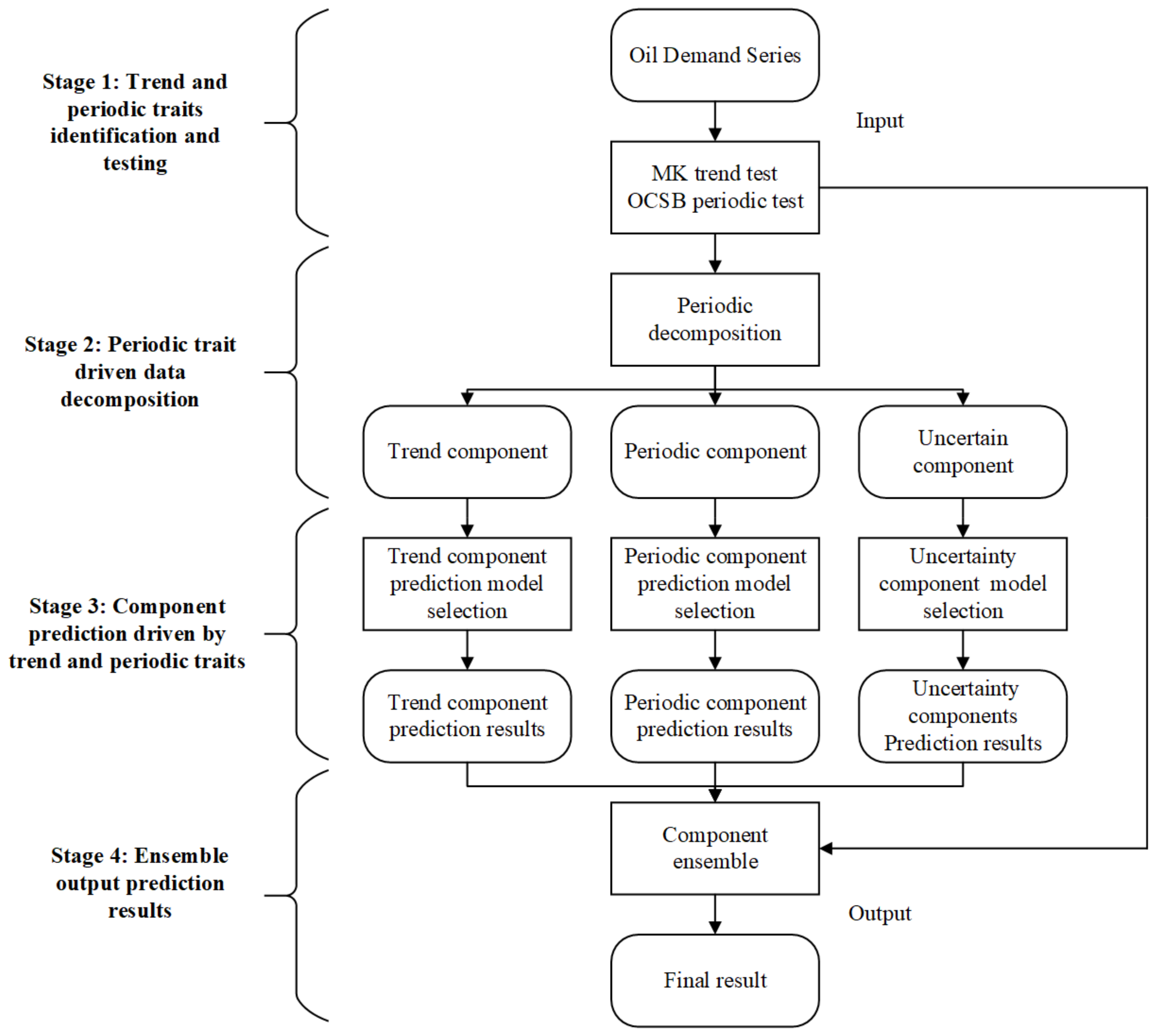
3. Trend- and Periodicity-Trait-Driven Decomposition-Ensemble Forecasting Model

In terms of the trend trait and periodicity trait of gasoline demand data, this paper proposed a trend- and periodicity-trait-driven decomposition-ensemble forecasting model to improve the prediction accuracy of gasoline demand, and the general theoretical framework is illustrated in Figure 1. In the proposed model, the trend and periodicity test of the gasoline demand data were first tested. In terms of the periodicity trait, the gasoline demand data were then decomposed into three components, i.e., trend, periodicity, and uncertainty components, by the periodic decomposition method. Subsequently, the component prediction model is selected in terms of the specific traits of the trend, periodic, and uncertain components so as to reflect the driving effect of the trend and periodicity characteristics on the prediction of gasoline demand.

As shown in Figure 1, the proposed trend- and periodicity-trait-driven decomposition-ensemble prediction model consists of four main stages, which are elaborated below.

Stage 1: Trend and periodicity trait identification and testing

Due to the influence of the economic and social environment and other factors, gasoline demand data has relatively regular cyclical fluctuations every year. Furthermore, due to the growth of car ownership, gasoline demand data has an obvious upward trend. Therefore, at this stage, the OCSB test is used as the main method for the periodic trait, and the MK test is used as the main method for the trend trait of the gasoline demand data.

Stage 2: Periodicity-trait-driven data decomposition

In terms of the test results of the periodicity trait of the gasoline demand data in the previous stage, seasonal decomposition is selected as the main decomposition method to reduce the difficulty of modeling. Thus, the original gasoline demand data were decomposed into three components: trend, periodicity, and uncertainty. Specifically, in the series of seasonal decomposition methods, the X11 seasonal decomposition method [19] is selected, and the strategy of additive decomposition is adopted. This method can decompose the original time series data into the trend component $T_t$, seasonal (periodic) component $S_t$, and residual term (uncertainty) component $R_t$, fully reflecting the data characteristics of each component.

Stage 3: Component prediction driven by trend and periodic traits

According to the specific data traits of each component obtained in Stage 2, the appropriate prediction model was selected for each component prediction with different data traits. For example, a linear regression (LR) model can be used as a prediction model for trend components with small fluctuations because it has the characteristics of stability predicting. For the cyclical component, the seasonal autoregressive integrated moving average (SARIMA) model with seasonal difference operators can therefore be used as a predictive model for component data with periodic or seasonal traits. Because neural networks can approximate any relationship and the neural network family model can be used as a prediction model for the uncertainty components with the complexity trait.

Stage 4: Ensemble output prediction results

The prediction results of each component were obtained through the component prediction of the previous stage, and at this stage, it is necessary to select the appropriate ensemble method to further integrate the component prediction result. Specifically, in this stage, it is necessary to comprehensively consider the trend and periodicity traits of the gasoline demand data to construct the connection rules between the selection of the ensemble method and the data traits. According to the rules, the suitable ensemble method can be used for integrated prediction so as to obtain the final prediction result. Based on the cyclical trait of the gasoline demand data and the additive decomposition that was used in Stage 2, the strategy of additive integration was adopted at this stage.

In practical use, the four main stages of the proposed trend- and periodicity-trait-driven decomposition-ensemble forecasting method will be conducted step by step. In the first step, the trend and periodicity traits of gasoline demand data are tested by the MK and OCSB test methods. In the second step, according to the periodicity trait, the gasoline demand data were divided into three parts, i.e., trend, periodicity, and uncertainty components, by the periodic decomposition method. In the third step, the component prediction models are selected in terms of the specific traits of the trend, periodic, and uncertain components so as to reflect the driving effect of the trend and periodicity characteristics on the prediction of gasoline demand. In the final step, the three component forecasting results are aggregated into the ensemble output as the final prediction result for gasoline demand. Using the above steps, the proposed trend- and periodicity-trait-driven decomposition-ensemble forecasting method can be used in practical forecasting tasks.

4. Experimental Results

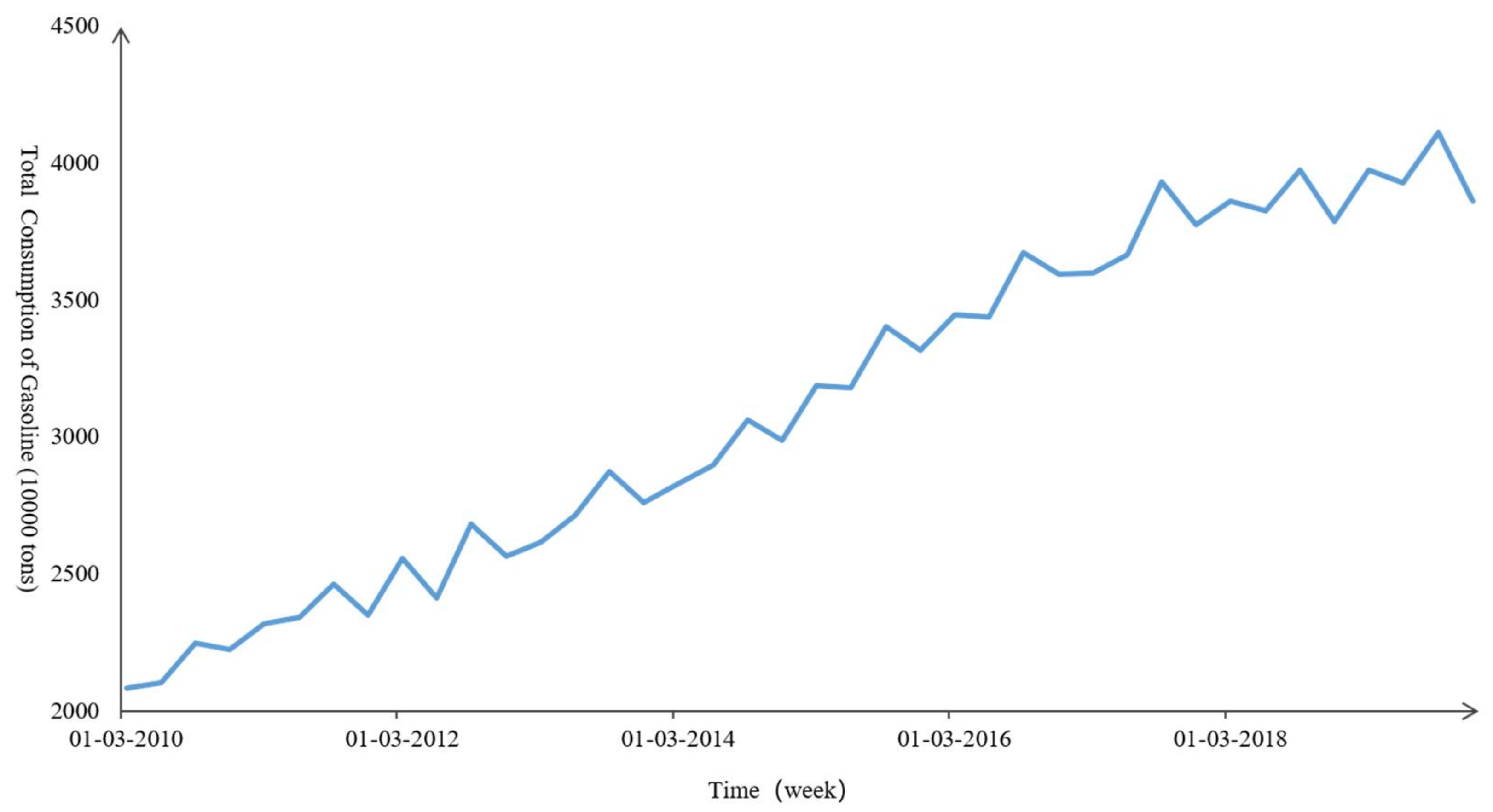
4.1. Data Description and Experimental Design

Since gasoline is a typical refined oil product with the largest consumption and the widest use range in China, this article selects the demand data for 93# gasoline as the research object to conduct predictive analysis. At the same time, for this research we selected the quarterly data of the total demand for 93# gasoline in China from Q1, 2010 to Q4, 2019 for the experiments. All of the data regarding gasoline demand were obtained from the Wind Database (http://www.wind.com.cn/), as shown in Figure 2.

For the raw data collected from the Wind database, the quarterly price data on gasoline demand needs to be preprocessed. Firstly, the missing values need to be handled. In this article, the missing values were filled in terms of the average of the previous quarter. After filling in the missing values, there were a total of 40 observations for the quarterly gasoline demand data, which covered from Q1, 2010 to Q4, 2019. At the same time, in order to eliminate the influence of data dimensions, this paper used the max-min normalization method to preprocess the data, and the normalization equation is expressed by

$$x_t^{\prime }=\frac{x_t-\min (x)}{\max (x)-\min (x)},\hspace{1em}\hspace{1em}t=1,2,3\dots k$$

(5)

where max(x) and min(x) are the maximum and minimum values in the sample data, respectively, x_t is the original sample, and $x_t^{\prime }$ is the normalized data. After normalization, all of the sample data were normalized to [0,1], which reduced the range of fluctuations in the data. It should be noted that the prediction results obtained based on the normalized data need to be denormalized to obtain the final prediction results.

In order to compare the prediction performance, seven single models, i.e., linear regression (LR), support vector regression (SVR), extreme learning machine (ELM), general regression neural network (GRNN), multilayer perceptron (MLP), extreme gradient boosting regression (XGB Regressor), and random forest (RF) were selected to predict gasoline demand. Subsequently, the above-mentioned typical single models were used as the component prediction technique to establish a trend- and periodicity-trait-driven decomposition-ensemble forecasting model and compare the prediction accuracy of all of the above models to select the optimal forecasting model. In order to statistically prove the superiority of the proposed decomposition-ensemble prediction model over other prediction models, this paper adopted a Diebold Mariano (DM) test [20] for this purpose. Finally, 80% of the sample data were used as the training set to train the model, and the remaining 20% of the data were used as the testing set to demonstrate the performance of the prediction models.

In order to test the effectiveness of the predictive model, this article uses three commonly used predictive indicators, mean absolute percent error (MAPE), root mean squared error (RMSE), and directional statistic (D_stat) to evaluate the prediction accuracy [16]. In particular, MAPE and RMSE are used to measure the of level accuracy, and D_stat is used to evaluate the accuracy of the direction predictions.

Considering that the gasoline demand forecast in the actual application of refined oil enterprises will affect the production-sales-stock plan of gasoline, short-term demand forecasting is often used to cope with the impact of instantaneous emergencies, and long-term demand forecasting is used to facilitate long-term planning. Therefore, this article forecasts future gasoline demand one-step, two-steps, three-steps, and four-steps in advance, i.e., the demand for the next quarter, second quarter, third quarter, and fourth quarter based on historical data. In particular, this article uses Python 3.7 (https://www.python.org/downloads/release/python-373/) to write codes that use the sitsmodels and scikit-learn modules to implement seasonal decomposition and prediction, respectively. By comparing the prediction results of each model, the optimal model can be selected for gasoline oil demand forecasting.

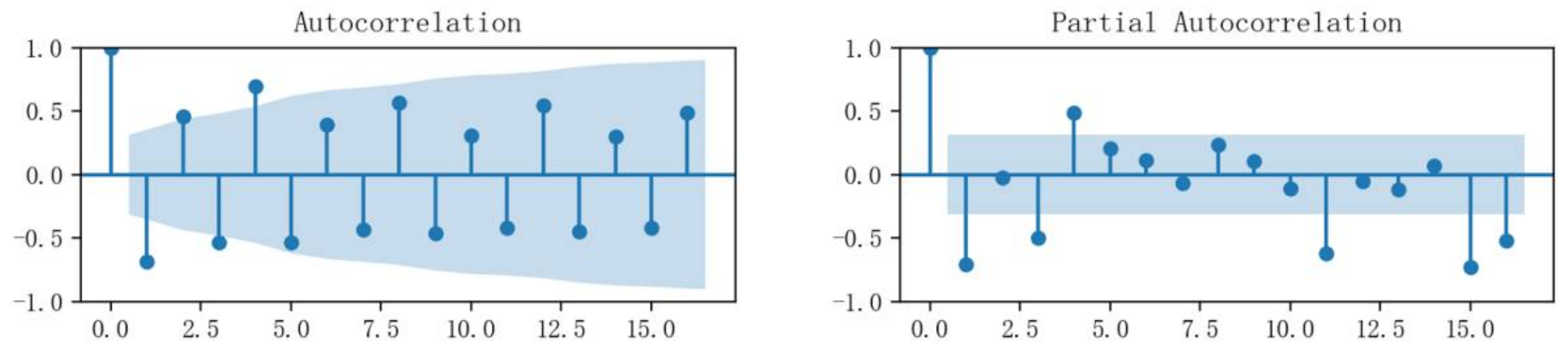
4.2. Data Trait Testing

Before using a specific prediction model, the gasoline demand data needed to be tested. First, the three steps of the MK test method were used to test the gasoline demand data and obtain the results $Z_c=8.35$, while at the 1% significance level, $Z_{\frac{1-\alpha }{21}}=2.576$, i.e., $\left|Z_c\right|>Z_{\frac{1-\alpha }{2}}$, and $Z_c$ is positive, indicating that the gasoline demand series data had a clear upward trend.

Next, the OCSB method was used to test the periodicity of gasoline demand with the 2nd, 3rd, 4th, and 5th-order lag analysis, the test results are shown in

Table 1. OCSB test results for gasoline demand data.

Data	Lag Order	Critic Value	t Statistic
Gasoline demand	2	−1.9520	−1.2621
	3	−1.9176	−2.800
	4	−1.8927	−1.2130
	5	−1.8735	−5.3354

Note: bold represents the significance of statistic test.

.

As can be seen from Table 1, for the gasoline demand data, both the 2nd and 4th order lags have seasonal unit roots, indicating that the gasoline demand series has Cyclical characteristics for two quarters (half a year) and four quarters (one year).

After the above statistical test, it was determined that the gasoline demand data had an obvious trend trait and the cyclical characteristics of half a year and one year, so it is reasonable to adopt some prediction models based on these two data traits.

As shown in Table 1, when the lag period of four provinces was four quarters, the correlation coefficient of the time series data were the largest. The test results demonstarted that the four time series data in Table 1 have cyclicity traits with a period of one year (four quarters).

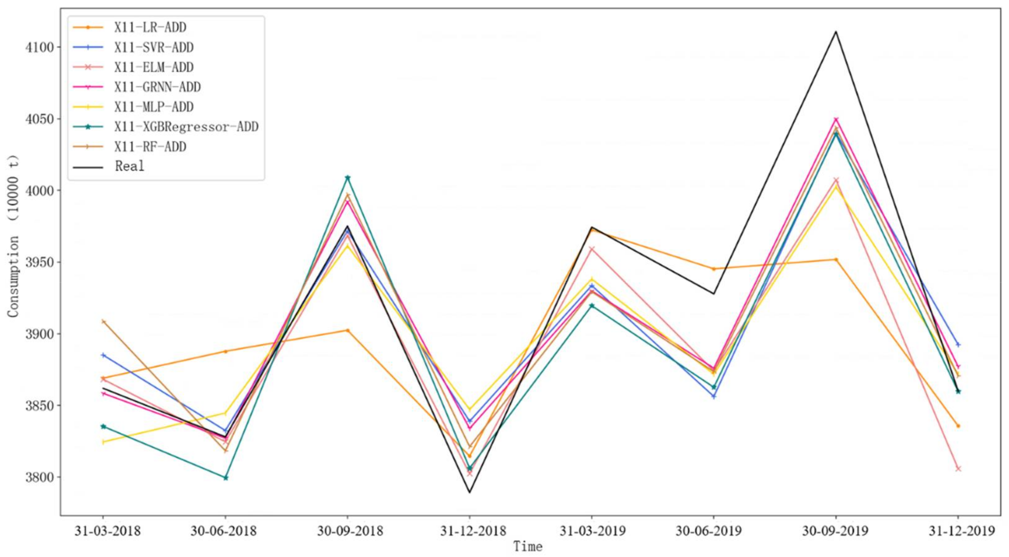
4.3. Experimental Results Analysis

In order to build a forecast model of the quarterly demand data for 93# gasoline, it is necessary first to determine a suitable lag period. For this purpose, the original time series of the 93# gasoline demand data were processed by the first-order difference, and then the ACF and PACF were calculated to determine the lag orders, as shown in Figure 3.

As can be seen from Figure 3, the optimal lag order is 2. After determining the lag order, one-, two-, three-, and four-step-ahead prediction of the gasoline demand data could be conducted. In order to compare the forecast results, various single models were first used to predict gasoline demand, and then the decomposition-ensemble forecasting methods were carried out based on the trend and cyclical traits of gasoline demand data.

According to the above experimental arrangement, seven single models were used, and the corresponding results of the gasoline demand forecasting are shown in

Table 2. Gasoline demand forecast results of seven single models.

Step Size	Metric	LR	SVR	ELM	GRNN	MLP	XGB	RF
One step	Dstat	0.6250	0.1250	0.7500	0.5000	0.2500	0.6250	0.6250
	MAPE	0.0240	0.0324	0.0222	0.0305	0.0264	0.0311	0.0244
	RMSE	112.6617	155.6208	94.9666	130.8414	117.6011	135.2791	112.6359
Two steps	Dstat	0.5000	0.7500	0.5000	0.5000	0.2500	0.7500	0.6250
	MAPE	0.0262	0.0415	0.0264	0.0295	0.0285	0.0300	0.0263
	RMSE	120.4158	196.1568	118.4198	138.8445	125.4783	139.5928	121.6565
Three steps	Dstat	0.5000	0.2500	0.5000	0.3750	0.3750	0.3750	0.3750
	MAPE	0.0361	0.0553	0.0330	0.0262	0.0251	0.0310	0.0300
	RMSE	146.9760	270.0291	136.0105	142.7566	122.1430	167.1368	156.0496
Four steps	Dstat	0.6250	0.6250	0.6250	0.5000	0.2500	0.5000	0.3750
	MAPE	0.0322	0.0767	0.0264	0.0322	0.0347	0.0336	0.0365
	RMSE	149.0826	332.0082	133.9106	143.4993	146.9649	149.6941	160.8493

Note: Bold represents the best results of different evaluation metrics.

.

As can be seen from Table 2, three interesting results can be found.

First of all, comparing the results of the one-step-ahead prediction horizontally, it was found that the extreme learning machine (ELM) models achieved the best results in three measurements, showing that the ELM model has a good fitness capability for short-term prediction. However, SVR models achieved the worst performance, which may be related to the choice of kernel functions, resulting in poor prediction stability.

Secondly, the longitudinal comparison of the prediction results for each step showed that with the growth of the predicted step, the prediction performance of each model decreased. In particular, the level of prediction accuracy for the SVR model decreased distinctly, while the level of prediction accuracy for the LR, MLP, and GRNN models were relatively stable with the increase in the predicted steps. The main reasons for this are that the stability of the linear regression model itself and the strong robustness of the neural network models are suitable for medium- to long-term forecasting tasks.

Finally, a comprehensive comparison of all of the prediction results shows that the ELM model achieved good results on both one-step-ahead and multi-step-ahead prediction tasks. In detail, the ELM obtained the best results in most metrics and all prediction steps. The main reasons for this are that the ELM model is actually a feed-forward neural network that has advantages over other shallow learning systems in terms of learning rate and generalization capabilities. Since decision-makers often need directional accuracy as a reference for policy-making, directional accuracy is an important consideration in multi-step-ahead forecasting. From Table 2, it can be seen that the ELM model with the best level of prediction accuracy achieved satisfactory directional accuracy of no less than 0.5 in the two-, three-, and four-step-ahead prediction, but such directional accuracy is far from supporting decision-making. Because a single model cannot fully learn the mapping relationships between historical data and future data when faced with complex data, the single models do not fit well with the actual data on gasoline demand. In particular, the general trend and volatility forecasting of gasoline demand data are not satisfactory. To solve this problem, this paper tries to use a decomposition-ensemble forecasting model based on the trend and periodicity traits to predict gasoline demand.

In the trend- and periodicity-trait-driven decomposition-ensemble prediction model, the decomposition method uses the X11 seasonal decomposition model, the component prediction method was uniformly selected from the above single models, and the ensemble method adopts additive (ADD) integration. Considering the above single models and decomposition-ensemble prediction models, the gasoline demand forecasting performance of the data-trait-driven decomposition-ensemble prediction model was explored. In order to compare the differences in the prediction accuracy between the ordinary decomposition-ensemble model without considering the characteristics of the component data and the data-trait-driven decomposition-ensemble model, this paper first tried to use the same predictive model for the different components and then tried to select different predictive models for different components in terms of the data traits to highlight the role of data-trait-driven modeling.

According to the above idea, the ordinary decomposition-ensemble prediction model, without considering the characteristics of the component data, was first used for the prediction analysis. Because the data component traits were not considered, the same predictive model was used for each decomposed component. Accordingly, Figure 4 shows the one-step-ahead (i.e., one quarter in advance) prediction performance of a decomposition-ensemble model with the same forecasting technique.

As can be seen in Figure 4, the prediction curve of the periodicity-trait-driven decomposition-ensemble model has a high degree of coincidence with the actual curve. In particular, GRNN as the component prediction method in the decomposition-ensemble model has the highest degree of coincidence, while the fitting curve of the LR component prediction technology model has a relatively large difference from the actual curve. The possible reason is that the LR model is conservative in predicting the maximum points, resulting in large prediction errors.

However, Figure 4 is only the one-step-ahead prediction. In order to compare the results of other prediction steps, this paper uses three indicators, D_stat, MAPE, and RMSE, to compare the prediction performance of the ordinary decomposition-ensemble prediction model, as shown in

Table 3. Gasoline demand forecasting results of the periodicity-trait-driven decomposition-ensemble model without considering the characteristics of the component data.

Step Size	Metric	X11-LR-ADD	X11-SVR-ADD	X11-ELM-ADD	X11-GRNN-ADD	X11-MLP-ADD	X11-XGB-ADD	X11-RF-ADD
One step	Dstat	0.6250	0.7500	0.7500	0.7500	0.6250	0.7500	0.7500
	MAPE	0.0115	0.0094	0.0134	0.0076	0.0107	0.0094	0.0088
	RMSE	66.8267	44.5502	72.2153	36.9964	51.9117	43.7886	39.2769
Two steps	Dstat	0.7500	0.7500	0.7500	0.7500	0.7500	0.7500	0.7500
	MAPE	0.0174	0.0091	0.0087	0.0087	0.0125	0.0103	0.0099
	RMSE	87.1333	41.8056	47.4198	40.2201	57.0031	45.2247	42.1567
Three steps	Dstat	0.7500	0.7500	0.6250	0.7500	0.7500	0.7500	0.7500
	MAPE	0.0156	0.0097	0.0134	0.0096	0.0132	0.0089	0.0121
	RMSE	79.8560	44.9304	64.0893	45.3510	61.2052	43.0854	50.6549
Four steps	Dstat	0.7500	0.7500	0.7500	0.7500	0.7500	0.7500	0.7500
	MAPE	0.0109	0.0087	0.0078	0.0078	0.0092	0.0089	0.0099
	RMSE	51.8899	43.1658	39.3814	40.1956	43.9967	40.4888	44.4135

Note: In the abbreviation of “X11-LR-ADD”, X11 is used for the decomposition method, LR is used as the prediction technique for each decomposed component, and ADD is adopted as the ensemble method. Bold represents the best results of different evaluation metrics.

.

Comparing the prediction results of single models in Table 2, the periodicity-trait-driven decomposition-ensemble forecasting model in Table 3 can effectively improve the performance of predicting gasoline demand. In terms of directional accuracy, most models achieved a directional accuracy of 0.75 for four different prediction steps. In the level of prediction accuracy, both RMSE and MAPE metrics improved significantly relative to the single models. In detail, the MAPE metrics on each prediction step of most single models was about 3%, and the MAPE of the proposed decomposition-ensemble prediction model was about 1%. In particular, the X11-GRNN-ADD model achieved the best results for different evaluation indicators in both one-step-ahead and two-step-ahead predictions. The main reason for this is that GRNN has excellent generalization capabilities, which can achieve good prediction performance in trending, periodic, and uncertain components. While X11-XGB-ADD and X11-ELM-ADD achieved the best results in the three-step-ahead and four-step-ahead predictions, respectively, indicating the superiority of these two methods in medium- and long-term forecasting.

The above analysis did not consider the data traits of the decomposed components, and the subsequent task is to use the proposed decomposition-ensemble model considering the decomposed component data traits for gasoline demand forecasting. Figure 5 shows the one-step-ahead prediction results of the proposed decomposition-ensemble model.

As can be seen from Figure 5, based on the data characteristics of each component, the proposed decomposition-ensemble model considering the decomposed component data traits can achieve better prediction results than the decomposition-ensemble model without considering the decomposed component data traits. From the graphical point of view, the coincidence of the fitted curve and the actual curve is significantly higher than that of Figure 4. In particular, the LR-SARIMA-GRNN model has the highest accuracy. The main reason is that the LR-SARIMA-GRNN model selects the most suitable prediction technique in terms of the specific data traits of different components. That is, a stable linear regression (LR) model was used for the smoother trend component, and an SARIMA with the seasonal trait was used for the periodic component, while the generalized regression neural network (GRNN) was used for the uncertain components with higher complexity, illustrating the effectiveness of data trait-driven modeling.

However, Figure 5 only presents one-step-ahead prediction results. In order to compare the results of other prediction steps, this paper used three indicators of D_stat, MAPE, and RMSE to compare the prediction results of the decomposition-ensemble prediction model considering the traits of the component data, as shown in

Table 4. Gasoline demand prediction results of the decomposition-ensemble model considering the traits of the component data.

Step Size	Metric	X11-LR-GRNN-XGB-ADD	X11-SVR-GRNN-ELM-ADD	X11-ELM-SVR-XGB-ADD	X11-LR-ELM-RF-ADD	X11-LR-SARIMA-GRNN-ADD
One step	Dstat	0.7500	0.7500	0.7500	0.7500	0.7500
	MAPE	0.0077	0.0096	0.0080	0.0092	0.0070
	RMSE	33. 8595	46.1372	38.1287	48.9500	32. 4460
Two steps	Dstat	0.7500	0.6250	0.7500	0.7500	0.7500
	MAPE	0.0083	0.0107	0.0079	0.0080	0.0100
	RMSE	33.9634	50.4139	34.4110	34.1056	41.2624
Three steps	Dstat	0.7500	0.6250	0.7500	0.7500	0.7500
	MAPE	0.0099	0.0123	0.0092	0.0102	0.0128
	RMSE	42.4172	54.3939	39.2703	45.5302	52.1904
Four steps	Dstat	0.7500	0.6250	0.7500	0.7500	0.7500
	MAPE	0.0099	0.0082	0.0096	0.0100	0.0116
	RMSE	47.2062	41.2325	48.8391	45.3290	49.0334

Note: In the abbreviation of “X11-LR-GRNN-XGB-ADD”, X11 is used for the decomposition method, LR, GRNN, XGB is used as the prediction technique for trend component, periodic (seasonal) component, and the uncertainty component, respectively, and ADD is adopted as the ensemble method. Bold represents the best results of different evaluation metrics.

.

Comparing Table 3 with Table 4, it can be seen that the proposed decomposition-ensemble model that selected different component prediction techniques in terms of the specific data traits was better than the ordinary decomposition-ensemble model that used the same prediction technology for different components. In terms of directional prediction accuracy, almost all of the models achieved a directional accuracy of 0.75. For the level of prediction accuracy, the RMSEs of almost all models were less than 50, while the MAPE was lower than 1%. In particular, the LR-SARIMA-GRNN model achieved the best results in the one-step-ahead prediction, which is a reflection of the effectiveness of the trait-driven modeling of the component data. In the multi-step-ahead prediction, the difference in the model performance of the models was very small. A detailed comparison of the prediction results for each prediction step can be found if the prediction step increases, the change in the prediction accuracy of each model is more stable and does not produce large fluctuations. This demonstrated that the proposed decomposition-ensemble models considering the component data traits were more robust than the ordinary decomposition-ensemble prediction models without considering the component data traits and single-prediction models.

In order to statistically judge the prediction difference between the various prediction models, the Diebold Mariano (DM) test method was used to determine the judgment. Since there are many single models and decomposition-ensemble models, the four models with the best results for two classes were selected for testing purposes. This article reported the DM test results for the one-, two-, three-, and four-step-ahead prediction of the 93# gasoline predictive models, as shown in

Table 5. DM test results of different models with one-step-ahead prediction.

Model	X11-SVR-GRNN-ELM-ADD	X11-ELM-ADD	X11-GRNN-ADD	ELM	SVR	MLP	LR
X11-LR-SARIMA-GRNN-ADD	−1.38 (0.17)	−2.31 (0.02)	−0.14 (0.89)	−4.50 (0.00)	−3.20 (0.00)	−4.09 (0.00)	−2.68 (0.01)
X11-SVR-GRNN-ELM-ADD		−2.23 (0.03)	1.45 (0.15)	−4.31 (0.00)	−3.12 (0.00)	−3.90 (0.00)	−2.29 (0.02)
X11-ELM-ADD			2.58 (0.01)	−1.62 (0.11)	−2.17 (0.03)	−1.96 (0.05)	−1.04 (0.30)
X11-GRNN-ADD				−3.82 (0.00)	−3.07 (0.00)	−4.19 (0.00)	−2.44 (0.01)
ELM					−1.37 (0.17)	−0.64 (0.52)	−0.29 (0.77)
SVR						0.91 (0.36)	0.81 (0.42)
MLP							0.30 (0.76)

,

Table 6. DM test results of different models with two-step-ahead prediction.

Model	X11-SVR-GRNN-ELM-ADD	X11-ELM-ADD	X11-GRNN-ADD	ELM	SVR	MLP	LR
X11-LR-SARIMA-GRNN-ADD	−0.26 (0.80)	−1.01 (0.31)	0.97 (0.33)	−4.05 (0.00)	−2.94 (0.00)	−3.54 (0.00)	−2.83 (0.00)
X11-SVR-GRNN-ELM-ADD		−1.53 (0.13)	1.13 (0.26)	−3.21 (0.00)	−2.92 (0.00)	−3.80 (0.00)	−2.16 (0.03)
X11-ELM-ADD			1.87 (0.06)	−2.96 (0.00)	−2.63 (0.01)	−3.31 (0.00)	−1.88 (0.06)
X11-GRNN-ADD				−3.60 (0.00)	−2.91 (0.00)	−4.17 (0.00)	−2.55 (0.01)
ELM					−1.18 (0.24)	−0.06 (0.95)	0.72 (0.47)
SVR						1.27 (0.20)	1.30 (0.19)
MLP							0.25 (0.80)

,

Table 7. DM test results of different models with three-step-ahead prediction.

Model	X11-SVR-GRNN-ELM-ADD	X11-ELM-ADD	X11-GRNN-ADD	ELM	SVR	MLP	LR
X11-LR-SARIMA-GRNN-ADD	0.10 (0.92)	1.54 (0.12)	−1.97 (0.05)	−4.35 (0.00)	−2.73 (0.01)	−1.83 (0.07)	−5.96 (0.00)
X11-SVR-GRNN-ELM-ADD		−2.37 (0.02)	1.58 (0.11)	−3.31 (0.00)	−2.79 (0.01)	−2.06 (0.04)	−3.94 (0.00)
X11-ELM-ADD			−0.34 (0.74)	−4.15 (0.00)	−2.84 (0.00)	−2.48 (0.01)	−4.91 (0.00)
X11-GRNN-ADD				−3.86 (0.00)	−2.82 (0.00)	−2.23 (0.03)	−5.06 (0.00)
ELM					−1.65 (0.10)	1.04 (0.30)	−1.33 (0.18)
SVR						2.51 (0.01)	1.18 (0.24)
MLP							−1.25 (0.21)

and

Table 8. DM test results of different models with four-step-ahead prediction.

Model	X11-SVR-GRNN-ELM-ADD	X11-ELM-ADD	X11-GRNN-ADD	ELM	SVR	MLP	LR
X11-LR-SARIMA-GRNN-ADD	1.03 (0.30)	0.67 (0.50)	1.29 (0.20)	−2.40 (0.02)	−4.65 (0.00)	−4.37 (0.00)	−3.09 (0.00)
X11-SVR-GRNN-ELM-ADD		−0.36 (0.72)	0.74 (0.46)	−2.16 (0.03)	−5.00 (0.00)	−5.54 (0.00)	−2.60 (0.01)
X11-ELM-ADD			0.61 (0.54)	−2.61 (0.01)	−4.76 (0.00)	−3.96 (0.00)	−3.20 (0.00)
X11-GRNN-ADD				−2.14 (0.03)	−4.89 (0.00)	−6.10 (0.00)	−2.57 (0.01)
ELM					−3.30 (0.00)	−0.40 (0.69)	−1.13 (0.26)
SVR						3.44 (0.00)	3.08 (0.00)
MLP							0.25 (0.81)

.

From the DM test results in Table 5, Table 6, Table 7 and Table 8, three important findings can be summarized.

(1)

Comparing the decomposition-ensemble prediction model with the single model, it can be found that at 90% confidence degree, the prediction performance of two different decomposition-ensemble models at each step is significantly better than the single models. The main reason for this is that the decomposition-ensemble framework can significantly reduce the complexity of modeling, thereby improving the prediction performance.

(2)

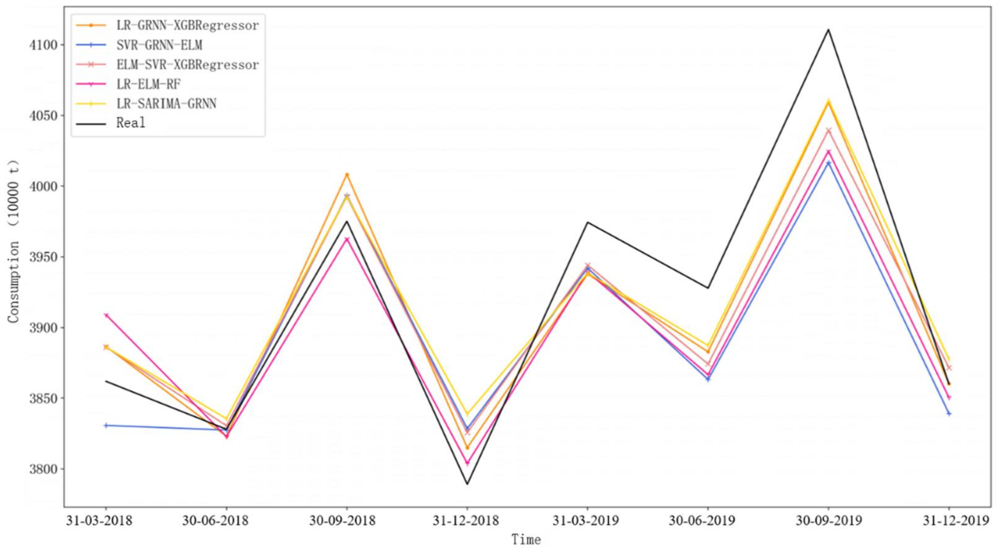
By comparing the ordinary decomposition-ensemble model without considering the component data traits with the component data-trait-driven decomposition-ensemble model, it can be found that the latter can significantly improve the prediction accuracy in short-term prediction. For example, in the first-step-ahead prediction, the X11-LR-SARIMA-GRNN-ADD model exhibits a better prediction performance than the other decomposition-ensemble models. This is because this model selects different prediction techniques in terms of the specific data traits of different components in turn, which effectively improves the results of component prediction. This also shows that data-trait-driven modeling plays a key role in gasoline demand forecasting.

(3)

Comparing the test results of the single models, the advantages and disadvantages of each model cannot be strictly determined from the statistical perspective when predicting shorter steps (one-step- and two-step-ahead), but for the longer steps (three-step- and four-step-ahead), significant differences are shown between the models. This is due to the fact that short-term predictions tend to achieve more accurate results than long-term predictions, and their difference in prediction performance is not significant. However, in long-term predictions, the predictive power of different forecasting models tends to vary greatly.

5. Discussion and Future Directions

In terms of the two typical data traits of gasoline demand, this paper constructs a novel trend- and periodicity-trait-driven decomposition-ensemble forecasting model. In this proposed forecasting model, the seasonal addition decomposition model called X11 is first adopted in terms of the periodicity-trait of gasoline demand. Then the linear model, seasonal model, and intelligent model were used for modeling the decomposed components with the traits of the trend, periodicity (i.e., seasonality), and uncertainty. Finally, the simple additive ensemble model was adopted based on the addition principle of decomposition. For verification purpose, the market demand for the 93# gasoline was used to confirm the effectiveness of the proposed trend- and periodicity-trait-driven decomposition-ensemble forecasting model. Through a comparative analysis of multiple experiments, four main conclusions can be obtained.

First, with the increase in prediction steps, the directional accuracy and the level of accuracy of the prediction results show a downward trend in both the single models and the decomposition-ensemble models. This shows that medium- or long-term predictions are more difficult than short-term ones, and thus in-depth research on medium- and long-term forecasting models is needed in the future. However, the decomposition-ensemble models show better prediction results than the single models, which also confirms the superiority of the decomposition-ensemble forecasting model [16].

Second, by comparing the single prediction models with the decomposition ensemble prediction model without considering the component data traits of the decomposed component, it can be found that the prediction accuracy of the latter is higher than that of the former. This shows that the decomposition-ensemble model can effectively reduce the complexity of modeling and improve prediction accuracy.

Third, by comparing the decomposition-ensemble model using the same prediction technique for all components and the decomposition-ensemble model using different prediction techniques for the different components, it was found that the prediction accuracy of the latter was much higher than that of the former. This reveals that selecting the appropriate prediction technique in terms of the specific data traits can effectively improve the prediction accuracy. This also confirms the effectiveness of the data-trait-driven modeling, which is consistent with the results of Tang et al. [6].

Finally, multiple experiments have found that the prediction accuracy of the trend- and periodicity-trait-driven decomposition-ensemble model proposed in this paper does not greatly decrease with the increase in the prediction step, which shows that the proposed decomposition-ensemble model is not only suitable for short-term predictions but also suitable for medium- and long-term forecasting with strong robustness. This implies that the proposed decomposition-ensemble model can provide strong support for the decision-makers of gasoline production enterprises to make short-term plans and long-term strategies at the same time.

However, there are still some issues that are worth discussing further.

(1)

The proposed decomposition-ensemble forecasting model is more suitable for time series data with the traits of trend and periodicity. However, if there are some other data traits such as long-memory, chaos, and fractality in the time series data, the proposed model may not be suitable for such time series data. Therefore, we will continue to explore the time series forecasting methods with other data traits.

(2)

Because gasoline demand is affected by multiple factors, it usually shows the coexistence of multiple data traits. This paper only considered two data traits; more data traits should be taken into account, which is also the direction to be studied in the future.

(3)

The proposed trend- and periodicity-trait-driven decomposition-ensemble forecasting model can also be applied to other markets, such as precious metal markets, chemical products markets, and other energy markets. Therefore, these new markets will be investigated in the future.

References

1. Azadeh, A.; Ghaderi, S.; Sohrabkhani, S. Annual electricity consumption forecasting by neural network in high energy consuming industrial sectors. Energy Convers. Manag. 2008, 49, 2272–2278. [Google Scholar] [CrossRef]
2. Bianco, V.; Manca, O.; Nardini, S. Electricity consumption forecasting in Italy using linear regression models. Energy 2009, 34, 1413–1421. [Google Scholar] [CrossRef]
3. Kucukali, S.; Baris, K. Turkey’s short-term gross annual electricity demand forecast by fuzzy logic approach. Energy Policy 2010, 38, 2438–2445. [Google Scholar] [CrossRef]
4. Wang, S.; Yu, L.; Tang, L.; Wang, S.Y. A novel seasonal decomposition based least squares support vector regression ensemble learning approach for hydropower consumption forecasting in China. Energy 2011, 36, 6542–6554. [Google Scholar] [CrossRef]
5. Tang, L.; Yu, L.; Wang, S.; Li, J.P.; Wang, S.Y. A novel hybrid ensemble learning paradigm for nuclear energy consumption forecasting. Appl. Energy 2012, 93, 432–443. [Google Scholar] [CrossRef]
6. Tang, L.; Yu, L.; He, K.J. A novel data-characteristic-driven modeling methodology for nuclear energy consumption forecasting. Appl. Energy 2014, 128, 1–14. [Google Scholar] [CrossRef]
7. Ahmad, A.S.; Hassan, M.Y.; Abdullah, M.P.; Rahman, H.A.; Hussin, F.; Abdullah, H.; Saidur, R. A review on applications of ANN and SVM for building electrical energy consumption forecasting. Renew. Sustain. Energy Rev. 2014, 33, 102–109. [Google Scholar] [CrossRef]
8. Tang, L.; Wang, Z.S.; Li, X.X.; Yu, L.; Zhang, G.X. A novel hybrid FA-based LSSVR learning paradigm for hydropower con-sumption forecasting. J. Syst. Sci. Complex. 2015, 28, 1080–1101. [Google Scholar] [CrossRef]
9. Akpinar, M.; Yumusak, N. Year Ahead Demand Forecast of City Natural Gas Using Seasonal Time Series Methods. Energies 2016, 9, 727. [Google Scholar] [CrossRef]
10. Ruiz, L.G.B.; Rueda, R.; Cuéllar, M.P.; Pegalajar, M.C. Energy consumption forecasting based on Elman neural networks with evolutive optimization. Expert Syst. Appl. 2018, 92, 380–389. [Google Scholar] [CrossRef]
11. Yu, L.; Zhao, Y.Q.; Tang, L.; Yang, Z.B. Online big data-driven oil consumption forecasting with Google trends. Int. J. Forecast. 2019, 35, 213–223. [Google Scholar] [CrossRef]
12. Yan, K.; Li, W.; Ji, Z.; Qi, M.; Du, Y. A Hybrid LSTM Neural Network for Energy Consumption Forecasting of Individual Households. IEEE Access 2019, 7, 157633–157642. [Google Scholar] [CrossRef]
13. Bedi, J.; Toshniwal, D. Deep learning framework to forecast electricity demand. Appl. Energy 2019, 238, 1312–1326. [Google Scholar] [CrossRef]
14. Liu, T.; Tan, Z.; Xu, C.; Chen, H.; Li, Z. Study on deep reinforcement learning techniques for building energy consumption forecasting. Energy Build. 2019, 208, 109675. [Google Scholar] [CrossRef]
15. Yu, L.; Ma, Y.; Ma, M. An effective rolling decomposition-ensemble model for gasoline consumption forecasting. Energy 2021, 222, 119869. [Google Scholar] [CrossRef]
16. Yu, L.; Ma, Y. A Data-Trait-Driven Rolling Decomposition-Ensemble Model for Gasoline Consumption Forecasting. Energies 2021, 14, 4604. [Google Scholar] [CrossRef]
17. Yue, S.; Pilon, P.; Cavadias, G. Power of the Mann–Kendall and Spearman’s rho tests for detecting monotonic trends in hy-drological series. J. Hydrol. 2002, 259, 254–271. [Google Scholar] [CrossRef]
18. Osborn, D.R.; Chui, A.; Smith, J.P.; Birchenhall, C.R. Seasonality and the order of integration for consumption. Oxf. Bull. Econ. Stat. 2010, 50, 361–377. [Google Scholar] [CrossRef]
19. Ladiray, D.; Quenneville, B. Seasonal Adjustment with the X-11 Method; Springer Science & Business Media: Berlin/Heidelberg, Germany, 2001. [Google Scholar] [CrossRef]
20. Diebold, F.X.; Mariano, R.S. Comparing predictive accuracy. J. Bus. Econ. Stat. 1995, 13, 134–144. [Google Scholar]
Figure 1. General framework of trend- and periodicity-trait-driven decomposition-ensemble forecasting method.
Energies 15 03553 g001
Figure 2. Chinese gasoline demand data from 2010 to 2019.
Energies 15 03553 g002
Figure 3. ACF and PACF results of 93# gasoline demand data.
Energies 15 03553 g003
Figure 4. One-step-ahead prediction results of the gasoline demand using the decomposition-ensemble model without considering the component data traits.
Energies 15 03553 g004
Figure 5. One-step-ahead prediction of gasoline demand using the decomposition-ensemble model considering the traits of the component data.
Energies 15 03553 g005