Bayesian Workflow and Hidden Markov Energy-Signature Model for Measurement and Verification

Abstract

A Bayesian data analysis workflow offers great advantages to the process of measurement and verification, including the estimation of savings uncertainty regardless of the chosen numerical model. However, it is still rarely used in practice, perhaps because practitioners are less familiar with the required tools. The present work documents a Bayesian methodology for the assessment of energy savings at the scale of a whole facility, following an energy-conservation measure. The first model, an energy signature commonly used in practice, demonstrates the steps of the Bayesian workflow and illustrates its advantages. The posterior distributions obtained by training this first model are used as prior distributions for a second, more complex model. This so-called “hidden Markov energy signature” model combines the energy signature with a hidden Markov model at an hourly resolution, and allows detection of occupancy. It has a large number of parameters and would likely not be identifiable without the Bayesian workflow. The results illustrate the advantages of the Bayesian methodology for measurement and verification: a probabilistic description of all variables, including predictions of energy use and savings; the applicability to any model structure; the ability to include prior knowledge to facilitate training complex models. Savings are estimated by the new hidden Markov energy-signature model with a much lower uncertainty than with a lower-resolution model. The highlights of the paper are twofold: it serves as a tutorial on Bayesian inference for measurement and verification; it also proposes a new flexible model structure for hourly prediction of energy use and occupancy detection.

1. Introduction

1.1. Motivation: Uncertainty Estimation in M&V

Measurement and Verification (M&V) is the assessment of energy savings gained from applying energy-conservation measures (ECM), for instance to a building. It is a necessary step for energy performance contracts, to prove that a contractual savings guarantee has been met. A robust assessment of energy savings is therefore an incentive for the implementation of ECMs by ensuring a stable environment for investment decisions.

The ASHRAE Guideline 14 [1] provides procedures for using measured preretrofit and postretrofit billing data for the calculation of energy, demand, and water savings. It formalises the main approaches for savings measurements: retrofit isolation, whole-facility and whole-building calibrated simulation approaches. These definitions were further elaborated by the International Performance Measurement and Verification Protocol (IPMVP) [2], published by the Efficiency Valuation Organisation: “Savings are determined by comparing measured consumption or demand before and after implementation of a program, making suitable adjustments for changes in conditions”. These adjustments are essential so that the estimation of savings represents the ECM rather than eventual changes in weather conditions and occupancy. They are calculated as follows:

• A numerical model is trained during a baseline observation period (before ECMs are applied);
• The trained model predicts energy consumption in the conditions of the reporting period (after energy-conservation measures);
• The adjusted energy savings are the difference between these predictions and the measured consumption of the reporting period.

There are several ways to classify the models used for M&V. The choice is often based on the available readings and their frequency [3]. Low-frequency (monthly or daily) data only allow the most simple models to be fitted: mean one-parameter model; two-parameter linear regression; three or more parameter change-point models with one or several slopes. These models have a very small number of parameters and a limited number of explanatory variables, although ordinary linear regression can easily include any number of them. Higher-frequency (hourly or minute) data open the possibility of using time-series models for a more precise estimation of savings, as we will show below. Alternatively, non-parametric models, or machine learning methods, are now popular as well. These include Gaussian Process models [4], Support Vector Machines [5], Gaussian Mixture and Artificial Neural Network models [6]. These methods are more flexible and can work on any type of meter, but lack physical interpretability.

Uncertainty quantification is essential to the M&V process, so that some confidence bounds can be displayed for energy savings [7]. The International Standards Organisation (ISO) Guide to the Expression of Uncertainty in Measurement (GUM) [8] provides instructions on expressing savings in probabilistic terms. However, the ASHRAE Guideline 14 [1] observes that standard approaches make it difficult to estimate the savings uncertainty when complex models are required:

“Savings uncertainty can only be determined exactly when energy use is a linear function of some independent variable(s). For more complicated models of energy use, such as change-point models, and for data with serially autocorrelated errors, approximate formulas must be used. These approximations provide reasonable accuracy when compared with simulated data, but in general it is difficult to determine their accuracy in any given situation.One alternative method for determining savings uncertainty to any desired degree of accuracy is to use a Bayesian approach.”

Bayesian statistics are increasingly popular [9] in all fields. A documented Bayesian M&V analysis was proposed by [10], who described its advantages and drawbacks. Advantages include:

• Bayesian models are probabilistic: uncertainty of all variables is automatically quantified.
• Bayesian models are universal and flexible. They can be very simple or very sophisticated, and are not restricted to the usual hypotheses of ordinary least squares regression.
• The Bayesian framework allows including prior information regarding expert knowledge.

1.2. Outline and Related Work

The present work applies Bayesian statistics to an example of the IPMVP Option C (whole building) approach. Two models are used and formulated in a Bayesian framework: a five-parameter change-point model with which M&V practitioners are familiar, and a more sophisticated model which combines this change-point model with a hidden Markov model for occupancy detection and hourly energy prediction. The point of the article is to demonstrate the universal applicability of Bayesian inference, and what it can bring to an M&V workflow:

• The ability to accurately estimate savings uncertainty, regardless of the model structure;
• The ability to use models of any complexity in order to account for occupancy, additional weather variables, and higher time resolution;
• The ability to validate complex models thanks to the regularisation features of prior distributions.

Section 2 starts with a general description of Bayesian data analysis and documents how it adapts to a M&V workflow. Section 3 presents the two models used in this study, and how conclusions from the simple one are the basis for training the second one. Section 4 presents the case study and the numerical tools used for calculations. Section 5 shows the results on training each baseline model in terms of parameter posterior distributions, posterior predictive distributions, disaggregation of energy savings, and occupancy detection.

This work is based on the author’s contribution to updating the IPMVP Uncertainty Assessment guide [11], where the Bayesian methodology is introduced. The same case study as described below, and the energy signature model, are used in this guide to illustrate the advantages of this method. The present paper extends this contribution with a second model which further demonstrates these advantages. The author’s webpage [12] will feature more tutorials and code examples on how to reproduce the results shown here.

2. A Bayesian Workflow for Measurement and Verification

2.1. Principles of Bayesian Data Analysis

The fundamentals of Bayesian inference and prediction are thoroughly explained in the book of Andrew Gelman [13]. A Bayesian model is defined by two components:

• An observational model $p\left(y\right|\theta )$, or likelihood function, which describes the relationship between the data y and the model parameters $\theta$. The choice of observational model is the same step as with any other M&V approach: ordinary linear regression, change-point models, polynomials, time-series models… There are no constraints on the number of parameters and independent variables.
• A prior model $p\left(\theta \right)$ which encodes eventual assumptions regarding model parameters, independently of the observed data. Specifying prior densities is not mandatory.

The target of Bayesian inference is the estimation of the posterior density $p\left(\theta \right|y)$, i.e., the probability distribution of the parameters conditioned on the observed data. As a consequence of Bayes’ rule, the posterior is proportional to the product of the two previously mentioned densities:

$$p\left(\theta \right|y)\propto p(\theta \left)p\right(y\left|\theta \right)$$

(1)

This formula can be interpreted as follows: the posterior density is a compromise between assumptions and evidence brought by data. The prior can be “strong” or “weak”, to reflect more or less confident prior knowledge. The posterior will stray away from the prior as more data is introduced.

In M&V applications, one is not only interested in estimating parameter values, but also the predictions $\tilde{y}$ of the observable during a new period (under conditions of the reporting period, or in “normalized” conditions). The distribution of $\tilde{y}$ is called the posterior predictive distribution, and is the density of $\tilde{y}$ conditioned on the observed data:

$$p\left(\tilde{y}\right|y)=\int p\left(\tilde{y}\right|\theta )p\left(\theta \right|y)\mathrm{d}\theta$$

(2)

Apart from the possibility to define prior distributions, the main specificity of Bayesian analysis is the fact that all variables are encoded as probability densities. The two main outcomes, the parameter posterior $p\left(\theta \right|y)$ and the posterior prediction $p\left(\tilde{y}\right|y)$, are not only point estimates but complete distributions which include a full description of their uncertainty.

Any model structure can be encoded into the observation function $p\left(y\right|\theta )$: change-point models, polynomials, models with categorical variables... Bayesian modelling, however, is much more flexible than standard regression methods such as the ordinary least squares method:

• Other distributions than the Normal distribution can be used in the observational model;
• Hierarchical modelling is possible: parameters can be assigned a prior distribution with parameters which have their own (hyper)prior distribution;
• Heteroscedasticity can be encoded by assuming a relationship between the error term and explanatory variables, etc.

Complex building energy simulation (BES) models can be used in a Bayesian framework, even though they are described by a large number of parameters and equations and cannot be summarised into a simple likelihood function $p\left(y\right|\theta )$. In order to apply Bayesian uncertainty analysis to a BES model, it is possible to first approximate it with a Gaussian process (GP) surrogate model. This process is based on the seminal work of [14], and is often denoted “Bayesian calibration”, although Bayesian modelling is not restricted to GP regression. As opposed to the manual adjustment of building energy-model parameters, Bayesian calibration explicitly measures uncertainty in calibration parameters and model predictions [15]. The reader is referred to [4,16,17] for examples of GP models used for M&V.

Except in a few convenient situations, the posterior distribution is not analytically tractable. In practice, rather than finding an exact solution for it, it is estimated by approximate methods. The most popular option for approximate posterior inference is Markov Chain Monte Carlo (MCMC) sampling methods [13]. A MCMC algorithm returns a series of simulation draws $\left({\theta }^{\left(1\right)},...,{\theta }^{\left(S\right)}\right)$ which approximate the posterior distribution, provided that the sample size is large enough.

$${\theta }^{\left(s\right)}\sim p\left(\theta \right|y)$$

(3)

where each draw ${\theta }^{\left(s\right)}$ contains a value for each of the p parameters of the model.

$${\theta }^{\left(s\right)}={\left({\theta }_1,...,{\theta }_p\right)}^{\left(s\right)}$$

(4)

This allows the posterior distribution of each individual parameter to be studied; moreover, pairwise distributions can be easily visualised for an investigation of eventual correlations between parameters, which may indicate low identifiability.

Since the posterior distribution is described by a finite (yet large) set of values, computing the statistics of any function h of the parameters (predictions, savings...) becomes straightforward. Because the series $\left({\theta }^{\left(1\right)},...,{\theta }^{\left(S\right)}\right)$ approximates the posterior distribution of $\theta$, then the series $\left(h\left({\theta }^{\left(1\right)}\right),...,h\left({\theta }^{\left(S\right)}\right)\right)$ approximates the posterior distribution of h. Specifically, the posterior predictive distribution $p\left(\tilde{y}\right|y)$ is approached by repeating model evaluations with the samples ${\theta }^{\left(s\right)}$ as inputs.

$$\begin{array}{cc}\hfill {\tilde{y}}^{\left(s\right)}& =p\left(\tilde{y}\right|\theta ={\theta }^{\left(s\right)})\hfill \end{array}$$

(5)

$$\begin{array}{cc}\hfill & \sim p\left(\tilde{y}\right|y)\hfill \end{array}$$

(6)

where each draw ${\tilde{y}}^{\left(s\right)}$ contains a value for each of the T data points of the prediction period.

$${\tilde{y}}^{\left(s\right)}={\left({\tilde{y}}_1,...,{\tilde{y}}_T\right)}^{\left(s\right)}$$

(7)

As a consequence, each individual data point i has a posterior predictive distribution approximated by the set ${\tilde{y}}_i^{\left(s\right)}$.

2.2. A Bayesian M&V Workflow

The following workflow describes the reporting period basis, or “avoided energy consumption” approach, of the IPMVP. It is theoretically applicable to any class of model, and to either the retrofit isolation and the whole-building approaches. We assume that the measurement boundaries have been defined and that data $y_{\mathit{base}}$ and $y_{\mathit{repo}}$ have been recorded during the baseline and reporting periods, respectively.

• As with standard approaches, choose a model structure to describe the data with, and formulate it as an observation model. Formulate eventual “expert knowledge” assumptions in the form of prior probability distributions.
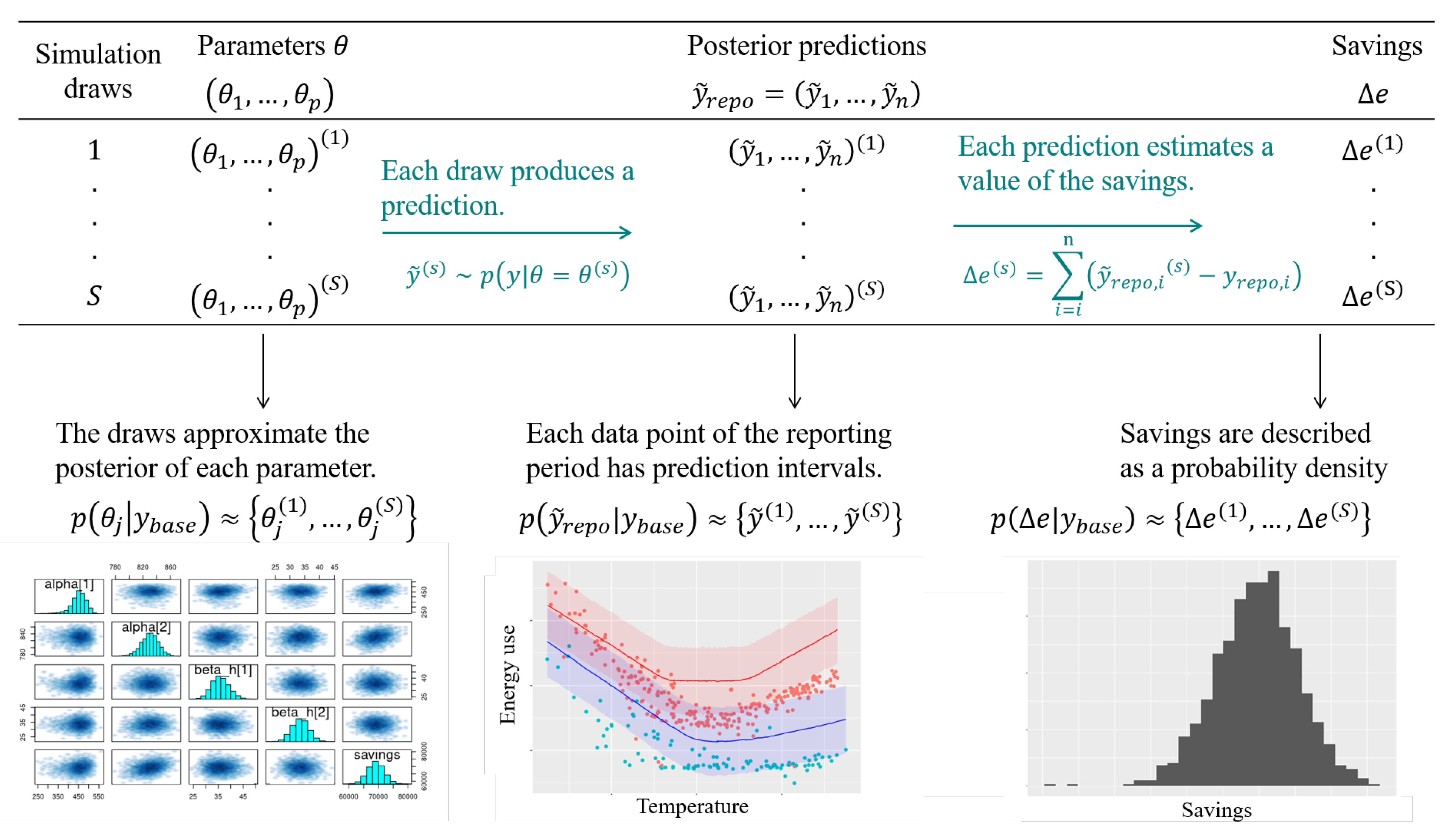
• Run a MCMC (or other) algorithm to obtain a set of samples $\left\{{\theta }^{\left(1\right)},...,{\theta }^{\left(S\right)}\right\}$ which approximates the posterior distribution of p parameters conditioned on the baseline data $p\left(\theta \right|y_{\mathit{base}})$. Validate the inference by checking convergence diagnostics: R-hat, ESS, etc.
• Validate the model by computing its predictions during the baseline period $p\left({\tilde{y}}_{\mathit{base}}\right|y_{\mathit{base}})$. This can be achieved by taking all (or a representative set of) samples ${\theta }^{\left(s\right)}$ individually, and running a model simulation ${\tilde{y}}_{\mathit{base}}^{\left(s\right)}\sim p\left(y_{\mathit{base}}\right|\theta ={\theta }^{\left(s\right)})$ for each. This set of simulations generates the posterior predictive distribution of the baseline period, from which any statistic can be derived (mean, median, prediction intervals for any quantile, etc.). The measures of model validation ($R^2$, net determination bias, t-statistic…) can then be computed either from the mean, or from all samples in order to obtain their own probability densities.
• Compute the reporting period predictions in the same discrete way: each sample ${\theta }^{\left(s\right)}$ generates a profile ${\tilde{y}}_{\mathit{repo}}^{\left(s\right)}\sim p\left(y_{\mathit{repo}}\right|\theta ={\theta }^{\left(s\right)})$, and this set of simulations generates the posterior predictive distribution of the reporting period.
• Since each reporting period prediction ${\tilde{y}}_{\mathit{repo}}^{\left(s\right)}$ can be compared with the measured reporting period consumption $y_{\mathit{repo}}$, we can obtain S values for the energy savings $\Delta e$, the distribution of which approximates the posterior probability of savings.

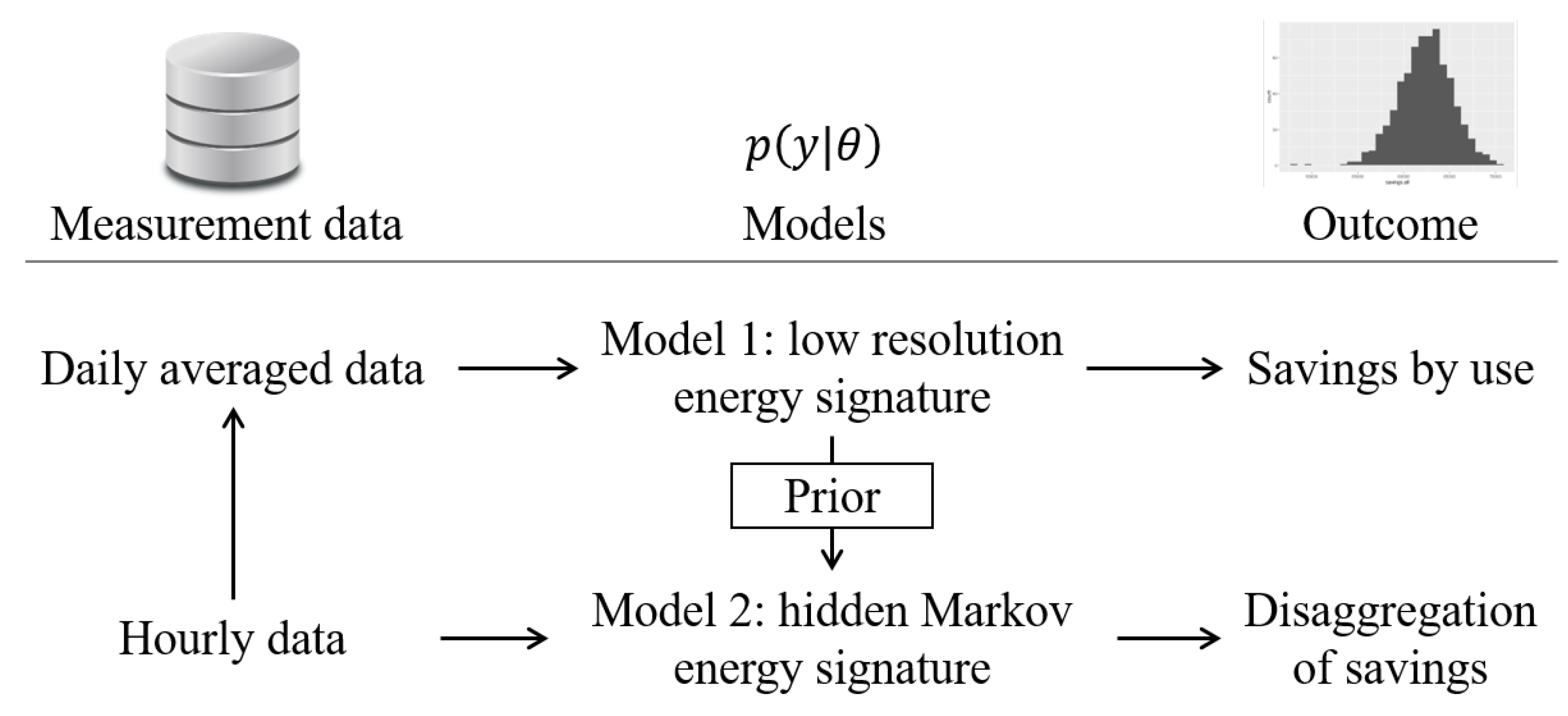
Steps 2, 4, and 5 of this description are illustrated by Figure 1.

In a “normalised savings” workflow, a numerical model is trained on both the baseline and the reporting period data. Each trained model then predicts the energy consumption during a period of normalised conditions, and savings are estimated by comparing these predictions.

3. Models

A typical Bayesian analysis of a dataset involves more than a single model. The common practice is to start with simple models, using low-resolution data and a few explanatory variables, then move on to a more detailed description of phenomena with more complex models and more parameters. Lessons learned from simpler models are used as prior functions into the next models [13]. This workflow is summarised on Figure 2 and applied below.

Hourly energy consumption data are first resampled into a daily resolution in order to train a first model based on the energy signature method. This first training follows the workflow described in Section 2.2, and its outcome is an estimation of energy savings and their uncertainty. These savings are also disaggregated with the level of detail allowed by this simple model. In a second step, the original higher-resolution data train a more detailed model. Posterior distributions obtained from training the first model are used here as prior, which facilitates training a complex structure. The outcome is a more detailed disaggregation of energy savings.

3.1. Model 1: Energy Signature Model for Low Resolution Data

Energy signature (ES) models assume a linear dependency of the heating (and/or cooling) energy consumption with the ambient air temperature, but only below (or above) a certain threshold. They often have a better fit than ordinary linear regression because they include a sort of regime switching.

The five-parameter ES, illustrated on Figure 3, decomposes the total energy consumption E of a building into three parts: heating, cooling, and base use. Heating and cooling are then assumed to be linearly dependent on the ambient temperature $T_a$, and only turned on conditionally on two threshold temperatures $T_1$ and $T_2$, respectively.

$$E=E_0+H_1{\left(T_1-T_a\right)}^{+}+H_2{\left(T_a-T_2\right)}^{+}$$

(8)

where $E_0$ is the temperature-independent energy use; $H_1$ and $H_2$ are the slopes in the heating and cooling ranges. The “+” exponent indicates that a term is only included if it is positive. This model is a piece-wise linear regression model, where the switching points $T_1$ and $T_2$ can be identified along with the other parameters. The slopes $H_1$ and $H_2$ can be interpreted as the heat-transfer coefficient of the envelope during heating and cooling seasons, respectively.

Equation (8) is the non-probabilistic formulation of the ES model. In probabilistic terms, we suppose that the data y (energy use) follow a Normal distribution around this mean value, with a constant standard deviation $\sigma$:

$$p\left(y\right|\theta ,T_a)=N\left[E_0+H_1{\left(T_1-T_a\right)}^{+}+H_2{\left(T_a-T_2\right)}^{+},\sigma \right]$$

(9)

Equation (9) is the likelihood function of our model, i.e., the conditional probability of y given the parameters $\theta$ and ambient temperature $T_a$. The model actually has six parameters: $\theta =\left\{E_0,T_1,T_2,H_1,H_2,\sigma \right\}$. The ambient temperature $T_a$ is the only explanatory variable. In a Bayesian framework, considering the uncertainty $\sigma$ as an unknown variable is common and easily implemented. Heteroscedasticity, a non-constant variance of errors, is also straightforward.

Data should be averaged over long enough (at least daily) sampling times because of the steady-state assumption: each energy use measurement is considered independent of its previous value.

The appeal of the energy-signature model is that the only data it requires are energy meter readings and outdoor air temperature. The large sampling time means that fast fluctuations of energy use are smoothed out, and no detailed modelling of user behaviour is required. Many improvements have been proposed to the original ES model, such as the possibility of including linear and non-linear energy use dependency on several variables: outdoor temperature, wind and solar irradiation [18].

Our own improvement of the ES model is based on a hidden Markov model with a higher time resolution: hourly instead of daily. This will allow a better accounting for the building occupancy in the M&V adjustment process.

3.2. Model 2: Hidden Markov Energy Signature Model for High Resolution Data and Occupancy Detection

Most of the data recorded by monitoring buildings are time series: sequences taken at successive points and indexed in time. The ES model described above deals with data that were aggregated with low enough frequency that successive values of the outcome variable could be considered independent from each other, and only dependent on explanatory variables. This aggregation, however, comes with a significant loss of information, since all dynamic effects are smoothed out. Dynamic models, including time-series models, allow the dependent variable to also be influenced by its own past values.

In a hidden Markov model (HMM), a sequence of T observed variables $y_t$ is generated by a sequence of categorical state variables $z_t\in \left\{1,\cdots ,K\right\}$. These hidden states are a Markov chain, so that $z_t$ is only dependent on $z_{t-1}$. This principle is illustrated by Figure 4.

The primary use of HMMs in building energy simulation is for identifying and modelling occupancy [19]. The hidden variable $z_t$ may denote a binary state of occupancy or a finite number of occupants; the observed output $y_t$ may denote any measurement impacted by occupancy: environmental sensors, smart meters, cameras, infrared sensors... There is a vast amount of literature on occupancy detection and estimation from different types of data and methods. The reader is referred to the review of Chen et al. [20] for a more comprehensive insight.

A HMM is defined by:

• A sequence of hidden states $\left\{z_t\right\}\in {\mathbb{N}}^T$, each of which can take a finite number of values: $z_t\in \left[1,...,K\right]$.
• An observed variable $\left\{y_t\right\}\in {\mathbb{R}}^T$
• An initial probability ${\pi }_0$ which is the likelihood of each state at time $t=0$. ${\pi }_0$ is a K-simplex, i.e., a K-vector which components sum to 1.
• A $K\times K$ one-step transition probability matrix $\mathbf{A}\left(t\right)=\left(a_{ij}\left(t\right)\right)$ so that

  $$a_{ij}\left(t\right)=p\left(z_t=j|z_{t-1}=i\right)$$

  is the probability at time t for the hidden variable to switch from state i to state j. Like ${\pi }_0$, each row of $\mathbf{A}\left(t\right)$ must sum to 1.
• Emission probabilities $b_i\left(y_t\right)=p\left(y_t\right|z_t=i)$, i.e., the probability distribution of the output variable given each possible state.

The transition probabilities $\left(a_{ij}\left(t\right)\right)$ are shown here as functions of time because they can be formulated as parametric expressions of external observed variables, such as the time of the day or weather variables. The Markov chain is then called inhomogeneous. Inhomogeneous transition probability matrices can capture occupancy characteristics at different time instances [21,22] and thus encode occupancy dynamics: a higher probability of people entering the building at a certain time of the day, or if the outdoor temperature is high, etc.

Training a HMM means finding the set of parameters $\theta$ that best explain the observations. The parameters define the transition $a_{ij}$ and emission $b_i$ probability functions, and eventually the initial state ${\pi }_0$. Training can be performed by in least two ways: the first option is to compute the likelihood function with the forward algorithm, and to perform its direct numerical maximisation. The second option is the Baum–Welch algorithm, which is a special case of the expectation-maximisation algorithm: it alternates between a forward–backward algorithm for the expectation step, and an updating phase for the maximisation step. A trained HMM can then be used to predict states and future values of the outcome variable. The estimation of the most likely state sequence given the observations is called decoding:

$$z_{0:T}^{*}={\mathrm{argmax}}_{z}p\left(z_{0:T}\right|y_{0:T})$$

(10)

and can be achieved using the Viterbi algorithm.

Many interesting models can be built upon the HMM structure by using custom functions for the transition $a_{ij}\left(t\right)$ and emission probabilities $b_i\left(y_t\right)$.

One of the possible extensions is autoregressive hidden Markov models [23] or Markov switching models (MSM) [24]. Similar to a HMM, an MSM is defined by a matrix of transition probabilities $\left(a_{ij}\left(t\right)\right)=p\left(z_t=j|z_{t-1}=i\right)$ whose terms can be conditioned on explanatory variables (time, day, weather...), and by emission probabilities. Rather than being only conditioned on $x_t$, the emission probability of an MSM is a function of previous observations in an autoregressive process. The MSM can be trained with the same Baum–Welch algorithm and decoded with the same Viterbi algorithm as an HMM: the structure of the algorithms is unchanged because $y_t$ is conditionally independent on $x_{t-1}$ given $x_t$ and $y_{t-1}$.

Here, we propose another extension of the HMM structure called the hidden Markov energy signature (HMES) model. It is a HMM where the emission probability functions are ES models:

• The energy use $y_t$ of a building at time t follows a different ES model for each possible occupancy state $z_t\in \left[1,...,K\right]$. This is how we allow the parameters of the ES model $\left\{E_0,T_1,T_2,H_1,H_2,\sigma \right\}$ to depend on the occupancy.

  $$b_i\left(y_t\right)=p\left(y_t\right|\theta ,T_a,z_t=i)=N\left[E_{0,i}+H_{1,i}{\left(T_{1,i}-T_a\right)}^{+}+H_{2,i}{\left(T_a-T_{2,i}\right)}^{+},{\sigma }_i\right]$$

  (11)
• The occupancy state at each time t is unknown, and described by a hidden Markov chain. We define a transition probability matrix for each hour of the day h and day of the week d

  $$a_{ij}(h,d)=p\left(z_{h,d}=j|z_{h-1,d}=i\right)$$

  (12)

This formulation can be described as follows: at every hour h and day d, the building has a probability $a_{ij}(h,d)$ to switch from the occupancy state i to state j. Then, if the building is in the occupancy state i, then its energy use follows one of K possible ES models $b_i\left(y_t\right)$.

If K is the number of possible states, this model may have up to $24\times 7\times K(K-1)+6K$ unknown parameters. This high number of parameters is typical of inhomogeneous Markov chains. Several assumptions can be made to reduce this number: we will not look for different occupancy patterns for all 7 days of the week, but will rather only separate weekends and working days. An additional method is described by [24]: transition probabilities can be described by continuous functions over time, which drastically reduces the number of parameters regardless of the time-step size of measurements within a day.

Bayesian inference will facilitate training the HMES model despite its high number of parameters: informative prior distributions can be provided for each element of the transition matrices. For instance, we strongly suspect office buildings to be vacant on the weekends and at night. Furthermore, prior distributions for the parameters of the separate ES models will be based on the posterior distributions obtained by the first ES model.

4. Case Study and Tools

4.1. Case Study

This example is based on an open dataset shared by the Lawrence Berkeley National Laboratory on the Open Energy Initiative platform (https://data.openei.org/submissions/603, accessed on 5 November 2018).

The dataset is called “Hourly energy consumption and outdoor air-temperature data for 11 commercial buildings (office/retail)”. It contains 11 files for seven buildings. Two of these buildings, buildings 6 and 7, have been monitored for three years: before, during, and after implementation of ECMs. This example will focus on Building 6, a 20,000 ft${}^2$ office building located in Richland, WA, USA.

The available data are the hourly total energy consumption and outdoor air temperature. There is no available information on the nature of the ECMs and on the type of HVAC systems, appliances, and primary energy used for heating, cooling, and other uses. Energy uses are not monitored in separate sub-meters, but aggregated in a single meter.

Figure 5 displays a first look at the data during the “Pre” period (the year 2009) of Building 6. Figure 5a, shows that the hourly energy consumption is highly dependent on the time of day and on the day of the week: the building is only occupied during business hours and working days. The daily energy-use shown on Figure 5b confirms this separation of working days and weekends, and suggests a dependency on the ambient temperature, which justified our choice for the energy-signature model described in Section 3.1.

Data will be labelled “Year 1”, “Year 2” and “Year 3”. Year 1 is 2009, before ECM, the baseline period. Years 2 and 3 are 2010 and 2011, respectively, two separate reporting periods during which savings will be evaluated.

4.2. Tools

MCMC methods, Gaussian processes, and other methods for posterior approximation are implemented in several software platforms. Two free and well-documented examples are: Stan [25], a platform for statistical modelling which interfaces with most data-analysis languages (R, Python, Julia, Matlab); pyMC3, a Python library for probabilistic programming. The present work uses Stan and R. The code for both models will be provided in the Appendix A.

Commonly used MCMC algorithms, such as Metropolis–Hastings or Gibbs sampler [13], are inefficient in high dimension because of their random walk behaviour. The Hamiltonian Monte Carlo (HMC) algorithm, implemented in Stan, suppresses this issue by exploiting the curvature of the posterior distribution to guide the Markov chain along regions of high-probability mass, which provides an efficient exploration of the typical set [26,27]. Applications of HMC to the calibration of building energy models include whole-building simulation [15] and state-space models [28].

Convergence diagnostics are an essential step after running an MCMC algorithm for a finite number of simulation draws. It is advised to have several chains run in parallel in order to compare their distributions. The similarity of estimates between chains is assessed by the R-hat convergence diagnostic [29]. The second diagnostic is the effective sample size (ESS), an estimate of the number of independent samples from the posterior distribution. Once trained, a model may be validated with the same metrics as in a standard M&V approach: $R^2$, NDB, CV-RMSE, F-statistic, etc.

5. Results and Discussion

5.1. Es Model: Bayesian M&V with Daily Resolution

Based on the insight of the data shown on Figure 5, two ES models were trained on the baseline data (year 1): one for working days and one for weekends.

5.1.1. Posterior Distributions

The posterior distributions of the model’s parameters are summarised by their mean and standard deviation in

Table 1. Summary of ES training results on the baseline period: mean and standard deviation of posterior distributions. “neff” (effective sample size) and “Rhat” are two MCMC convergence diagnostics.

	Weekends				Working Days
	Mean	sd	neff	Rhat	Mean	sd	neff	Rhat
$E_0$ (kW)	18.7	1.59	1654	1.00	34.6	0.53	4869	1.00
$T_1$ (C)	9.81	1.47	2073	1.00	6.5	0.81	3860	1.00
$T_2$ (C)	16.21	4.50	982	1.01	15.8	3.89	7578	1.00
$H_1$ (kW/K)	1.50	0.145	5324	1.00	1.39	0.120	5205	1.00
$H_2$ (kW/K)	0.626	0.393	685	1.01	1.22	0.140	5409	1.00
$\sigma$	4.29	0.162	7578	1.00

. The standard deviation is lower than the mean for all parameters. Only the two parameters dealing with the cooling during weekends ($T_2$ and $H_2$) have a R-hat slightly above one, due to having fewer data allowing their precise estimation.

Figure 6 shows another insight into the posterior distribution, approximated by a finite but large set of samples. The diagonal plots confirm that most parameters have a nearly Gaussian posterior, although the distributions of the threshold temperatures $T_1$ and $T_2$ are slightly non-symmetric. Approximate Bayesian inference by MCMC is indeed not restricted to identifying normal distributions. Moreover, the off-diagonal plots of Figure 6 show the pairwise relationships between parameters in the joint posterior distribution: there is some degree of correlation between some of them.

5.1.2. Posterior Predictive Distributions

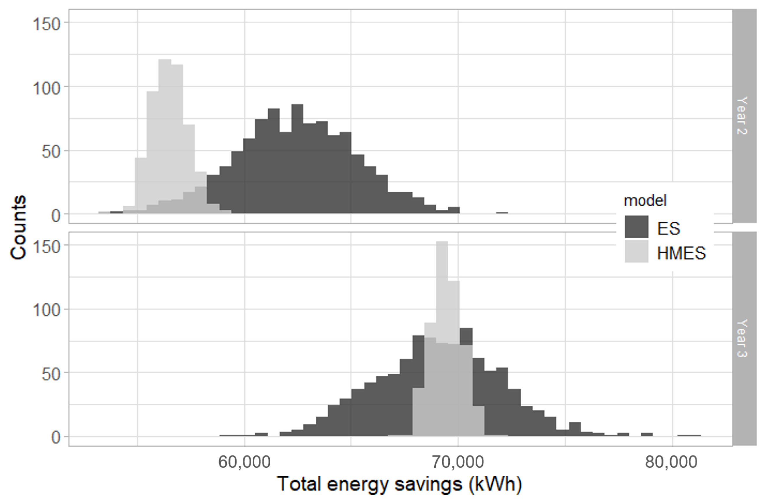
As explained in Section 2.1, the second result of Bayesian inference is the posterior predictive distribution. Just as the joint-parameter posterior distribution $p\left(\theta \right|y)$ is approximated by a large set of samples $\left({\theta }^{\left(1\right)},...,{\theta }^{\left(S\right)}\right)$, the posterior predictive distribution $p\left(\tilde{y}\right|y)$ is approximated by a set $\left({\tilde{y}}^{\left(1\right)},...,{\tilde{y}}^{\left(S\right)}\right)$ so that:

$${\tilde{y}}^{\left(s\right)}\sim N\left[E_0^{\left(s\right)}+H_1^{\left(s\right)}{\left(T_1^{\left(s\right)}-T_a\right)}^{+}+H_2^{\left(s\right)}{\left(T_a-T_2^{\left(s\right)}\right)}^{+},{\sigma }^{\left(s\right)}\right]$$

(13)

All statistics of the predictions can therefore be analysed by running the computer model with a representative number of samples from the parameter posterior distribution. Figure 7 shows the prediction mean and 95% prediction intervals by the model fitted on baseline data.

Figure 7a shows the prediction during the baseline period for comparison with the training data. Most data points are contained within the 95% prediction intervals as expected. Figure 7b compares data from one of the reporting periods (year 2) with the predictions of the baseline-trained model during the same period. The difference between the two gives the energy savings, adjusted on weather data, according to the “reporting period basis” M&V protocol.

5.1.3. Savings

Since predictions come in the form of a probability density for each data point of the reporting period, energy savings $\Delta e$ are also expressed as a probability density, approached by a large set of samples:

$$\begin{array}{cc}\hfill \Delta e^{\left(s\right)}& =\sum _{\mathrm{i}=1}^T\left({\tilde{y}}_{\mathrm{repo},\mathrm{i}}^s-y_{\mathrm{repo}})\right)\hfill \end{array}$$

(14)

$$\begin{array}{cc}\hfill & \sim p(\Delta e|y_{\mathrm{base}},y_{\mathrm{repo}})\hfill \end{array}$$

(15)

where T is the number of data points in the reporting period, $y_{\mathrm{repo}}$ is the reporting-period data, and ${\tilde{y}}_{\mathrm{repo},\mathrm{i}}^s$ is one sample of predictions.

In addition to estimating total energy savings, the method allows disaggregating them with the same level of detail as the ES model. We can separately assess the reduction of energy consumption during working days and weekends, and for the three uses: heating, cooling, and temperature-independent consumption. The latter disaggregation, however, requires training the ES model on the reporting period data so that the three terms of Equation (13) can be decomposed as well.

The disaggregated savings are shown on Figure 8 for both years of the reporting period.

• There is a large overlap between estimated savings during both reporting years, suggesting that no additional ECM was performed between years 2 and 3.
• Most energy savings after the ECM are found on the “base” (temperature-independent) energy consumption, and mostly during working days.
• The probability of cooling savings is centred around zero for weekends and working days during both years.
• The heating savings are likely negative during working days: this energy consumption is likely to have slightly increased after the ECM. This may be caused by a rebound effect, as it occurs when the building is occupied.

These findings are already quite informative and highlight the advantages of Bayesian inference well. We would now like to assess whether the HMES model allows a higher time-resolution in the description of energy savings.

5.2. HMES Model: High Resolution Bayesian M&V with Occupancy Detection

The HMES model described in Section 3.2 may work with any predefined number of states K which denote levels of occupancy. In this work we have chosen $K=3$ in order to represent the building as vacant, partially occupied, and fully occupied. A search for the best number of states has not been attempted.

5.2.1. Posterior Distributions

The HMES model is a hidden Markov model with energy-signature models as its emission probability functions. Training it, therefore, results in the estimation of a set of energy-signature parameters for each state. The mean and standard deviation of their posterior distributions are summarised on

Table 2. Summary of HMES training results on the baseline period: mean and standard deviation of posterior distributions.

	State 1		State 2		State 3
	Mean	sd	Mean	sd	Mean	sd
$E_0$	16.7	0.29	26.0	0.39	33.6	0.40
$T_1$	7.39	0.24	13.5	0.29	14.0	0.23
$T_2$	2.01	0.81	7.46	0.32	5.98	0.27
$H_1$	1.27	0.026	1.29	0.028	1.69	0.031
$H_2$	0.24	0.012	1.43	0.029	1.64	0.020
$\sigma$	3.98	0.031

. The base consumption $E_0$ of states 1 and 3 match the values obtained with the ES model during weekends and working days: this suggests that these states indeed denote a vacant and occupied building, respectively. The slopes $H_1$ and $H_2$ (see Figure 3) also seem to match, although there is no significant difference between states. Only the threshold temperatures show more variation. In particular, the cooling-threshold temperature of state 1 is difficult to interpret because there are few data allowing its estimation.

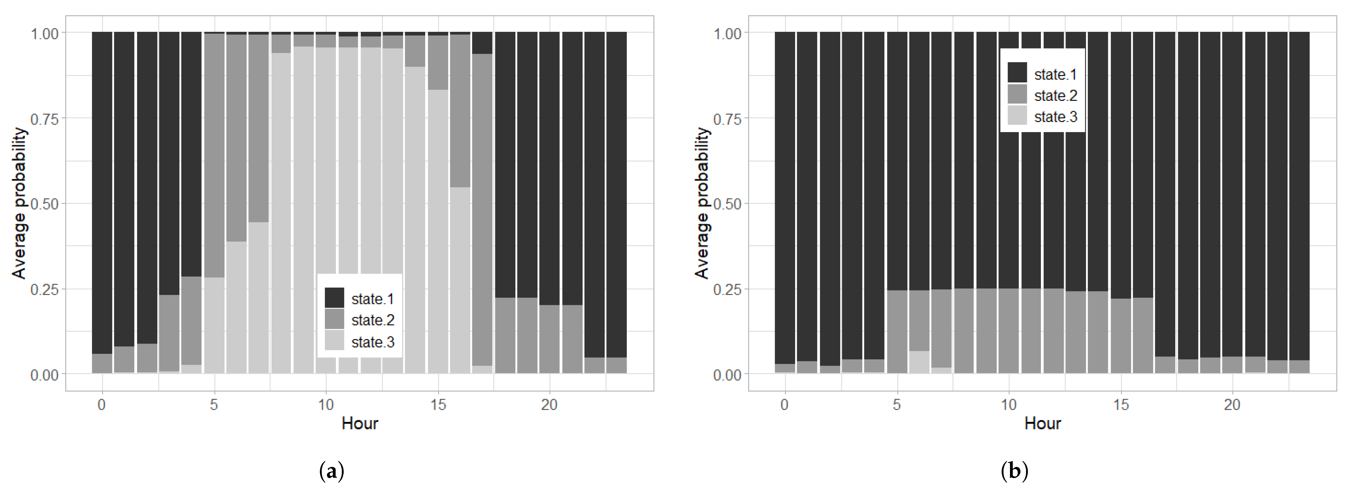
5.2.2. Occupancy Detection

Along with the parameters of K separate energy-signature models, the parameters of the HMES model also include the definition of the transition probability matrix. The components of this $K\times K$ matrix are defined by:

$$a_{ij}(h,w)=p\left(z_{h,w}=j|z_{h-1,w}=i\right)$$

(16)

where h is the time of day (24 possible values) and w is a categorical variable separating weekends from working days (two possible values). The total number of values in the transition matrices is therefore $24\times 2\times K\left(K-1\right)=288$. This high number of parameters is normally difficult to identify unless the data are very large, but the Bayesian framework allows us to avoid this problem: strong priors can be imposed in order to formulate our assumptions on occupancy: the building is very likely to be vacant (state 1) at night and on weekends, and very likely to be occupied otherwise (state 3).

The estimated average probability of each state at each time of the day is shown on Figure 9a (working days) and Figure 9b (weekends). We may observe a very high probability for the building to be vacant (state 1) most of the time in the weekends, and from 18:00 to 5:00 during the working days. The hours of maximal occupancy probability are 8:00 to 16:00 on working days, and state 2 of “partial occupancy” seems likely in between.

5.2.3. Savings

The main target of this M&V workflow is the estimation of total energy savings by a model trained on the baseline period, adjusted for the conditions of the reporting period. The ES model allowed this and even allowed some degree of savings disaggregation into energy uses. The next question is whether the HMES model offers any additional value to this matter, besides the already mentioned occupancy detection.

First, the HMES model is compared to the ES model in terms of estimation of total energy savings. The posterior distribution of total yearly energy savings is shown by Figure 10 during both years of the reporting period. A good overlap can be observed between the output of both models, especially during year 3, where the means of both distributions are close. The second observation concerns the width of posterior distributions: the HMES model offers much lower uncertainty in the estimation of energy savings.

The ES model allowed the disaggregation of energy savings by type (heating, cooling, and temperature independent) and by day (working days and weekends), as shown by Figure 8. The HMES model allows taking this disaggregation to the hourly resolution.

Figure 11 shows the hourly distribution of average energy savings by type, during the two reporting period years. As was already estimated by the ES model, the majority of energy savings during weekends are from the base energy use. During working days, “base” energy savings are significant while the building is vacant, and “cooling” savings are significant during opening hours. This does not match our previous observations from the ES model, which stated that heating and cooling savings were not significant. This suggest that more work is required to ensure the reliability of this disaggregation.

5.3. Drawbacks of a Bayesian Method and Limitations of This Work

Despite all its advantages, a Bayesian workflow has several drawbacks. Some of them were described by [10] and were also observed in the present case study.

The first practical disadvantage is the computational cost. A single MCMC run requires several thousands of iterations before convergence: calculations are much longer than with a regular curve-fitting tool. Parallelisation is limited to the number of chains running simultaneously, as each one cannot be parallelised further. For this reason, Bayesian models are difficult to implement to “big data” problems, but remain accessible to data that do not exceed a few gigabytes.

The second practical issue is the use of priors, which is a double-edged sword. On the one hand, a strong prior may facilitate the convergence of an otherwise non-identifiable model: without one, even a simple model such as the energy signature may have several solutions (several combinations of parameters) if data were insufficient to favour one. On the other hand, a strong prior may bring a subjective bias to the posterior, perhaps in contradiction with the data. A proper Bayesian workflow [26] encourages careful encoding of expert knowledge into prior distributions.

The HMES model is defined by a particularly large number of parameters. Convergence of posterior distributions was only successful by using conclusions from the first model, and spending time making a reasonable initial guess on the occupancy schedule of the building. This process is more time consuming than fitting a generic model template, but the outcome is also much more informative.

Both the ES and the HMES model used for this IPMVP Option C case study only rely on measurements of global energy meters at the building scale, and of outdoor air temperature. The results could easily be improved by any additional explanatory variable made available by monitoring: solar irradiance, wind, indoor temperature, sub-meters... On the other hand, due to the lack of dedicated sensors, our estimation of occupancy could not be validated with any baseline data.

6. Conclusions

This paper is a contribution to improving current practices of measurement and verification for the estimation of energy savings and their uncertainty following an energy-conservation measure.

The first input of this work is the Bayesian workflow for M&V. While this is not the first Bayesian M&V study, we chose to document the “avoided consumption” workflow for a typical IPMVP option C case. As the Bayesian framework describes all variables as probabilities, it directly estimates the uncertainty of energy savings regardless of model structure. The estimation of uncertainty is not bounded by the usual hypotheses of ordinary linear regression. This flexibility was illustrated by implementing a change-point model for which uncertainty estimation by standard methods is not trivial. Another advantage of the Bayesian method, in the author’s opinion, is its simplicity despite an initial learning curve.

The flexibility of the Bayesian method and the ability to specify parameter prior distributions allow experimentation with higher model complexity. Complex models may return more detailed inferences at the cost of lower identifiability, which may be mitigated by the proper use of informative priors.

The second input of this work, therefore, is the HMES model, which combines a hidden Markov model and the energy signature (five-parameter change-point) model with an hourly resolution. Like a HMM, it describes the occupancy of a building as a finite number of possible states, and assigns a different ES model for each state. Besides predicting energy use, it detects the probability of occupancy at every time of the day. The estimation of energy savings by this model were found more precise than with the daily resolution energy signature. The work also demonstrates the ability to disaggregate energy savings into the three uses described by both models: heating, cooling, and other uses.

The study focused on an IPMVP Option C (whole-building approach) example, but the same workflow can be applied to retrofit isolation (options A and B) due to the use of simple regression models. To the author’s knowledge, however, there has been no documented example of a Bayesian whole-building calibrated simulation (Option D) approach. In this approach, savings are determined through detailed simulation of the energy use of the whole facility, or of a sub-facility. It is particularly suitable if no historical energy data are available before the energy-conservation measure. Performing a Bayesian Option D study could be possible by applying the so-called Bayesian calibration [14] through a Gaussian process surrogate model. This is certainly a promising outlook for future work.

References

1. ASHRAE. Measurement of Energy, Demand, and Water Savings; ASHRAE Guideline 14-2014; ASHRAE: Atlanta, GA, USA, 2014. [Google Scholar]
2. Efficiency Valuation Organization. International Performance Measurement and Verification Protocol—Core Concepts; Efficiency Valuation Organization: Washington, DC, USA, 2022. [Google Scholar]
3. Granderson, J.; Touzani, S.; Custodio, C.; Sohn, M.D.; Jump, D.; Fernandes, S. Accuracy of automated measurement and verification (M&V) techniques for energy savings in commercial buildings. Appl. Energy 2016, 173, 296–308. [Google Scholar]
4. Heo, Y.; Zavala, V.M. Gaussian process modeling for measurement and verification of building energy savings. Energy Build. 2012, 53, 7–18. [Google Scholar] [CrossRef]
5. Dong, B.; Cao, C.; Lee, S.E. Applying support vector machines to predict building energy consumption in tropical region. Energy Build. 2005, 37, 545–553. [Google Scholar] [CrossRef]
6. Zhang, Y.; O’Neill, Z.; Dong, B.; Augenbroe, G. Comparisons of inverse modeling approaches for predicting building energy performance. Build. Environ. 2015, 86, 177–190. [Google Scholar] [CrossRef]
7. Walter, T.; Price, P.N.; Sohn, M.D. Uncertainty estimation improves energy measurement and verification procedures. Appl. Energy 2014, 130, 230–236. [Google Scholar] [CrossRef] [Green Version]
8. ISO. Guide to the Expression of Uncertainty in Measurement (GUM); ISO: Geneva, Switzerland, 2008. [Google Scholar]
9. Lira, I. The GUM revision: The Bayesian view toward the expression of measurement uncertainty. Eur. J. Phys. 2016, 37, 025803. [Google Scholar] [CrossRef]
10. Carstens, H.; Xia, X.; Yadavalli, S. Bayesian energy measurement and verification analysis. Energies 2018, 11, 380. [Google Scholar] [CrossRef] [Green Version]
11. Efficiency Valuation Organization. Uncertainty Assessment for IPMVP; Efficiency Valuation Organization: Washington, DC, USA, 2019. [Google Scholar]
12. Rouchier, S. Building Energy Statistical Modelling. 2021. Available online: https://buildingenergygeeks.org/ (accessed on 5 May 2022).
13. Gelman, A.; Carlin, J.B.; Stern, H.S.; Dunson, D.B.; Vehtari, A.; Rubin, D.B. Bayesian Data Analysis; CRC Press: Boca Raton, FL, USA, 2013. [Google Scholar]
14. Kennedy, M.C.; O’Hagan, A. Bayesian calibration of computer models. J. R. Stat. Soc. Ser. B 2001, 63, 425–464. [Google Scholar] [CrossRef]
15. Chong, A.; Menberg, K. Guidelines for the Bayesian calibration of building energy models. Energy Build. 2018, 174, 527–547. [Google Scholar] [CrossRef]
16. Burkhart, M.C.; Heo, Y.; Zavala, V.M. Measurement and verification of building systems under uncertain data: A Gaussian process modeling approach. Energy Build. 2014, 75, 189–198. [Google Scholar] [CrossRef]
17. Maritz, J.; Lubbe, F.; Lagrange, L. A practical guide to Gaussian process regression for energy measurement and verification within the Bayesian framework. Energies 2018, 11, 935. [Google Scholar] [CrossRef] [Green Version]
18. Rasmussen, C.; Bacher, P.; Calì, D.; Nielsen, H.A.; Madsen, H. Method for scalable and automatised thermal building performance documentation and screening. Energies 2020, 13, 3866. [Google Scholar] [CrossRef]
19. Candanedo, L.M.; Feldheim, V.; Deramaix, D. A methodology based on Hidden Markov Models for occupancy detection and a case study in a low energy residential building. Energy Build. 2017, 148, 327–341. [Google Scholar] [CrossRef]
20. Chen, Z.; Jiang, C.; Xie, L. Building occupancy estimation and detection: A review. Energy Build. 2018, 169, 260–270. [Google Scholar] [CrossRef]
21. Andersen, P.D.; Iversen, A.; Madsen, H.; Rode, C. Dynamic modeling of presence of occupants using inhomogeneous Markov chains. Energy Build. 2014, 69, 213–223. [Google Scholar] [CrossRef]
22. Chen, Z.; Zhu, Q.; Masood, M.K.; Soh, Y.C. Environmental sensors-based occupancy estimation in buildings via IHMM-MLR. IEEE Trans. Ind. Inform. 2017, 13, 2184–2193. [Google Scholar] [CrossRef]
23. Murphy, K.P. Dynamic Bayesian Networks: Representation, Inference and Learning; University of California: Berkeley, CA, USA, 2002. [Google Scholar]
24. Wolf, S.; Møller, J.K.; Bitsch, M.A.; Krogstie, J.; Madsen, H. A Markov-Switching model for building occupant activity estimation. Energy Build. 2019, 183, 672–683. [Google Scholar] [CrossRef]
25. Stan Development Team. Stan Language Reference Manual, Version 2.22. Available online: https://mc-stan.org/users/documentation/ (accessed on 5 May 2022).
26. Betancourt, M. A conceptual introduction to Hamiltonian Monte Carlo. arXiv 2017, arXiv:1701.02434. [Google Scholar]
27. McElreath, R. Statistical Rethinking: A Bayesian Course with Examples in R and Stan; CRC Press: Boca Raton, FL, USA, 2016. [Google Scholar]
28. Lundström, L.; Akander, J. Bayesian calibration with augmented stochastic state-space models of district-heated multifamily buildings. Energies 2020, 13, 76. [Google Scholar] [CrossRef] [Green Version]
29. Vehtari, A.; Gelman, A.; Simpson, D.; Carpenter, B.; Bürkner, P.C. Rank-normalization, folding, and localization: An improved R for assessing convergence of MCMC. Bayesian Anal. 2021, 1, 1–28. [Google Scholar] [CrossRef]
Figure 1. Estimation of savings with uncertainty in an “avoided consumption” workflow. The probability distribution of any function of the model parameters can be approximated by a finite number of simulations.
Energies 15 03534 g001
Figure 2. Working with models of increasing complexity.
Energies 15 03534 g002
Figure 3. Energy signature model, also known as a five-parameter change-point model.
Energies 15 03534 g003
Figure 4. Variable dependency in a hidden Markov model. Grey nodes denote the observed output sequence; white nodes denote the hidden states. Hidden states are conditioned on each other, while each observation is only conditioned on the current state.
Energies 15 03534 g004
Figure 5. Insight of the data during the baseline period (year 1). (a) Hourly energy use during two weeks; (b) daily energy use during one year.
Energies 15 03534 g005
Figure 6. Visualisation of the joint posterior distribution: individual parameters (diagonal) and pairwise relationships (off-diagonal).
Energies 15 03534 g006
Figure 7. Comparison of measured data (dots) and model predictions (lines and areas). The coloured areas are the 95% prediction intervals of the baseline-fitted model. (a) Baseline data vs model prediction; (b) Reporting period data vs. prediction from baseline-fitted model.
Energies 15 03534 g007
Figure 8. Disaggregation of energy savings with the ES model.
Energies 15 03534 g008
Figure 9. Probability of each occupancy state by hour of day. (a) Working days; (b) weekends.
Energies 15 03534 g009
Figure 10. Comparison of total yearly savings estimated by both models.
Energies 15 03534 g010
Figure 11. Average energy savings by type of consumption and hour of day. (a) Working days; (b) weekends.
Energies 15 03534 g011