Bearing Fault Diagnosis under Time-Varying Speed and Load Conditions via Observer-Based Load Torque Analysis ^†

Abstract

Bearing fault is the most common failure in rotating machines, and bearing fault diagnosis (BFD) has been investigated using vibration, current, or acoustic signals. However, there are still challenges in some existing approaches. This study proposes a novel BFD method based on natural observer. Based on the analysis of the effects on the load torque signal caused by bearing faults in the permanent magnetic synchronous machine (PMSM), a modified natural observer was designed to reconstruct the load torque signal from electrical signals, acquiring a novel indicator without the additional sensor installed. Angular resampling was implemented to convert the non-stationary load torque signal into a stationary one to reduce the computational complexity. For full-auto diagnosis without human involvement, a threshold determination algorithm was also modified. Experimental validations were carried out under speed-varying and torque-varying conditions and were compared with phase current and q-axis current signals. The average signal-to-noise ratio (SNR) of the estimated load torque is about 8.65 times compared with the SNR of the traditional q-axis current. The effectiveness of the proposed method prior to the traditional PMSM bearing fault indicators is demonstrated by the order spectrum results.

1. Introduction

Fault diagnosis in electrical motors has become an widely researched field for life extension and cost savings. According to the distribution of failure within the electrical motors reported by survey papers, bearing faults are the most significant faults in the rotating electrical machines, accounting for 40% to 90%, which are dependent on the size and type of the machine [1]. In the Internet of Things (IoT) field, applications of electrical motors have been extremely ‘extended’, and supervising health conditions is a key to fast repair and precise maintenance [2,3,4,5]. Therefore, effective bearing fault diagnosis (BFD) methods are highly desired to detect bearing faults and replace them, in a timely manner, to prevent severe damage and disastrous consequences.

Bearing faults can be categorized into generalized roughness and single-point defects [6]. Since generalized roughness is relatively hard to be detected, researchers have focused more on single-point defects. Vibration monitoring techniques are the most widely researched and are proven to be effective [7,8,9]. On the other hand, researchers are focusing on motor current spectrum analyses (MCSA) [10], since the current sensors are necessary for metering, controls, protection purposes, and additional vibration sensors are not required [11].

In addition to vibration signals and MCSA, the most frequently used signal among all the manuscripts aimed at bearing fault diagnosis, researchers also developed encoder-based speed [12], Luenberger observer-based speed [13], and load torque [14]. Among these, load torque is a directly-induced physical quantity that involves bearing fault. Since the load torque sensor is not commonly used in industrial applications due to reliability and cost, load torque estimation based on a mathematical model is a cost-effective method for load torque construction.

Challenging operating conditions in the industry, including a constantly changing motor speed and load torque, require improving the unsatisfying performance of the traditional stationary signal process method. The frequency smearing phenomenon will obviously be observed in the power spectra of the motor current in the transient operating condition. Using the time–frequency signal processing algorithm, such as short-time Fourier transform (STFT) [15,16], Wigner–Ville distribution (WVD) [17,18], Wavelet Transform (WT) [19,20], and wavelet package decomposition (WPD) [21,22], the transient time domain information can be revealed in the spectrogram, and the information hidden in the frequency domain will not be buried by the frequency smearing phenomenon. For extracting fault-related information precisely in the time–frequency spectrogram, a novel ridge estimation method [23] is implemented in STFT spectrogram. A novel signal decomposition method [24] can decompose multiply time-varying signals one by one using a recursive framework embedded with an iterative algorithm.

Order tracking, besides time–frequency signal processing technology, is another effective algorithm that can be used to solve the frequency smearing phenomenon in transient operating conditions. Order tracking resamples the time domain non-stationary signals at a constant angle increment corresponding to the time-angle curve, calculates the new value using linear or cubic spline interpolation, and converts the time domain signals to the angular domain signals, which are stationary and much easier to be analyzed. As stated above, order tracking requires the information of the rotating angle, or the time-angle curve, for the resample implementation. Much research is devoted toward acquiring the rotating angle with high accuracy, to be free from tachometer installation, which can significantly reduce the cost and maintenance demand, and meet the limits of special applications. For example, STFT is used to track the fundamental component buried in the current signal and the phase information of the current signal will be used as an angular resampling baseline [25]. To synchronize sampling with the rotor position, an estimation of the rotor position obtained from the angle of the voltage vector is proposed, and the angle is obtained from a phase-locked loop synchronized with generator voltages [8]. In [26], the high frame-rate video camera is set for identification of the pre-marked rotating parts, to calculate the rotating angle by analyzing the captured video using the object tracking algorithm. The combination of the fast spectral kurtosis (SK) analysis together with the STFT can clearly lead to extract the instantaneous fault characteristic frequency (IFCF) using the spectral peak search algorithm based on the amplitude sum [27]. These simple and effective methods for non-stationary condition diagnoses in the BFD are proven to be effective by experiments.

In this paper, a novel BFD method for the permanent magnet synchronous machine (PMSM) is proposed. A natural observer [28] is modified for PMSM implementation to reconstruct the load torque signal from electrical signals. It is a universal electrical motor fault indicator since it can be reconstructed using the basic sensors mounted on the electrical motors and has better performance than the traditional indicators. The computational complexity of the non-stationary estimated load torque signal can be significantly reduced by the angular resample algorithm compared with those time–frequency representation algorithms. When analyzing the order spectra, a full-auto spectrum threshold-generating algorithm is proposed to get rid of the arbitrary decision made by humans. The bearing fault can be diagnosed under severe time-varying working conditions with high accuracy; human involvement is unnecessary.

This paper is constructed as follows. The model of the natural observer and the discussion on the modification are presented in Section 2. Section 3 presents the implementation of the proposed torque signal angular resample process and the full-auto spectrum threshold-generating algorithm. Section 4 validates the proposed method for the diagnosis of bearing fault under different operating conditions. Section 5 concludes the paper.

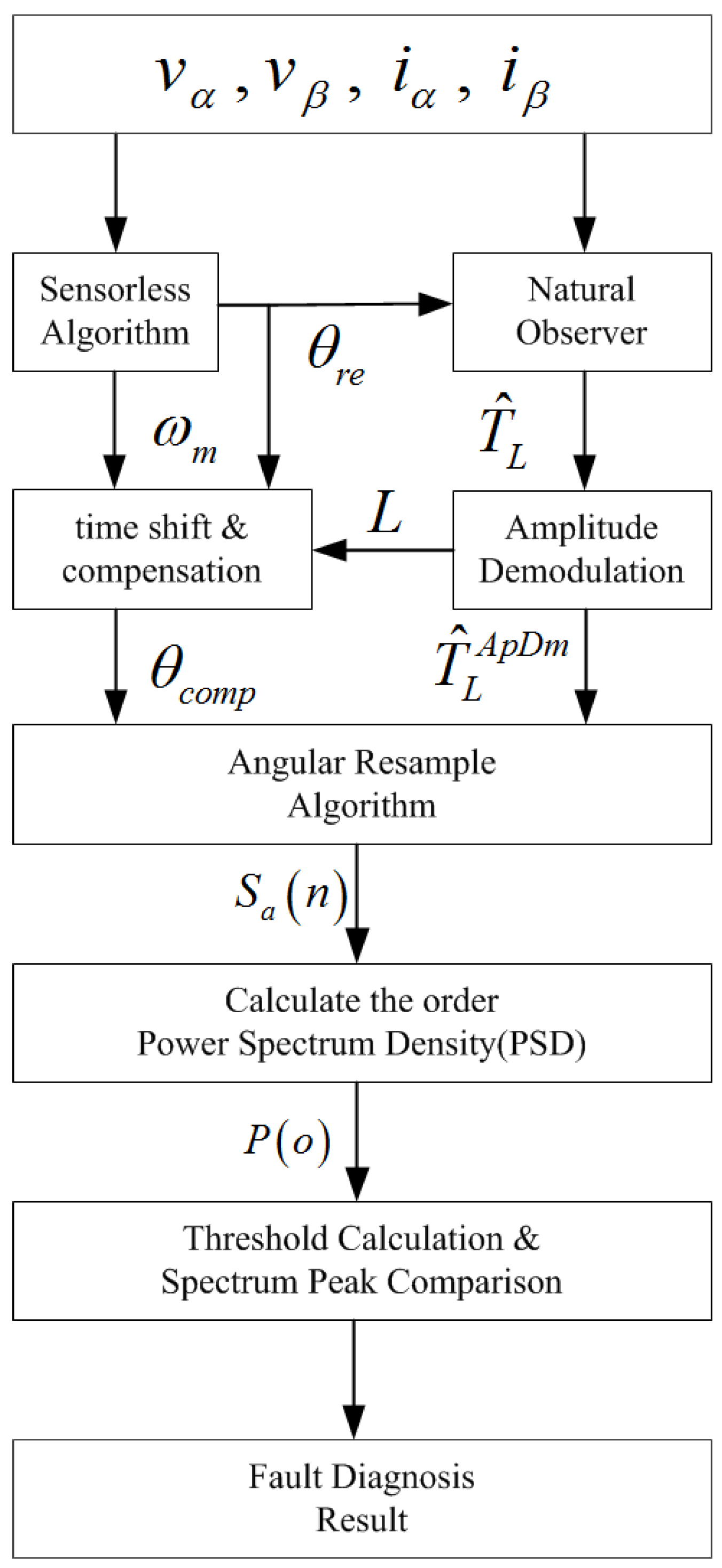
2. Mathematical Model of Modified Natural Observer

In this section, a modified natural observer is introduced for PMSM load torque observation.

The natural observer proposed in [28] is identical to the actual motor system model and has no external feedback to eliminate the influence caused by the noise of the measured signal. Since there is no feedback term, a parameter adaptation is essential for the natural observer to stabilize the system.

The original natural observer described in [28] was established in the orthogonal d–q frame, and was designed for DC motors and induction motors. The d–q frame is intrinsic in the control of DC motors, and in induction motors, the M-T frame is determined by the direction of the flux vector that is arbitrarily chosen. In the case of PMSM, the d–q frame should be aligned with the direction of the rotor magnet field. Therefore, if the optical encoder is not suitable to install, the position of the frame should be provided by the speed sensorless algorithm.

The position sensorless algorithm based on extended electromotive force (EEMF) described in [29] is applied to construct the d–q frame for the natural observer using the estimated angle position. The estimated speed will be used only for the speed sensorless control. The measured values $i_q$, $U_q$ and $i_d$ used in (1)–(10) can be obtained without the installed encoder.

The form of the natural observer is shown as follows:

$$\begin{array}{c}\hfill \frac{d}{dt}{\widehat{i}}_q=\frac{1}{L_q}(U_q-R_s{\widehat{i}}_q-L_d{i}_d{\widehat{\omega }}_e-\Psi {\widehat{\omega }}_e)\end{array}$$

(1)

$$\begin{array}{c}\hfill \frac{d}{dt}{\widehat{\omega }}_e=\frac{n_{pp}}{J_s}({\widehat{T}}_e-{\widehat{T}}_L)\end{array}$$

(2)

$$\begin{array}{c}\hfill {\widehat{T}}_e=\frac{3n_{pp}}{2}(\Psi {\widehat{i}}_q+(L_d-L_q)i_d{\widehat{i}}_q)\end{array}$$

(3)

where ${\widehat{i}}_q$ and ${\widehat{\omega }}_e$ are the estimation values of the q-axis current and electrical speed, ${\widehat{T}}_e$ and ${\widehat{T}}_L$ are the estimation values of the electrical magnetic torque and load torque, $R_s$$L_d$$L_q$$\Psi$$J_s$$n_{pp}$ are parameters of PMSM, standing for stator resistance, d-axis inductance, q-axis inductance, rotor flux, moment of inertia, and number of pole pairs, respectively. $U_q$ represents the input q-axis voltage. $i_d$ represents the actual value of the d-axis current.

The adaptive value ${\widehat{T}}_L$ will be adjusted using the active power error $\epsilon$ [30].

$$\begin{array}{c}\hfill {\widehat{T}}_L=k_p\epsilon +k_i\int \epsilon dt+k_d\dot{\epsilon }\end{array}$$

(4)

$$\begin{array}{c}\hfill \epsilon =|U_q^{\prime }|(i_q-{\widehat{i}}_q)\end{array}$$

(5)

where $k_p$, $k_i$, and $k_d$ are all positive parameters of the proportional integral derivative (PID) controller [31], and $|U_q^{\prime }|=|U_q|$.

The natural observer is constructed with only the actual value of the q-axis current $i_q$ and the actual value of the electrical speed ${\omega }_e$ being estimated as $\widehat{i_q}$ and ${\widehat{\omega }}_e$, and $i_d$ is directly used as its measured value. The error $\epsilon$ in (5) for adjusting the estimated load torque ${\widehat{T}}_L$ stands for the active power error, and should be calculated as

$$\begin{array}{c}\hfill {\epsilon }^{\prime }=|U_q^{\prime }|(i_q-{\widehat{i}}_q)+\left|U_d^{\prime }\right|(i_d-{\widehat{i}}_d)\end{array}$$

(6)

there exists the occasions that ${\widehat{i}}_d$ and ${\widehat{i}}_q$ do not simultaneously equal their actual values $i_d$ and $i_q$, respectively, while the error ${\epsilon }^{\prime }$ still becomes zero, e.g., the observer runs to a wrong steady point. This problem can be solved by equalizing the $i_d$ and the ${\widehat{i}}_d$ when designing the natural observer. The natural observer can also be downgraded from the nonlinear observer to a linear observer when ${\widehat{i}}_d$ is replaced by its true value $i_d$, and the complexity can be reduced.

The controllability, observability, and stability of the proposed natural observer will be discussed using the linear state-space equation form.

$$p\left[\begin{array}{c}{\widehat{i}}_q\\ {\widehat{\omega }}_e\\ {\widehat{T}}_L\end{array}\right]=\left[\begin{array}{ccc}-\frac{R_s}{L_q}& -\frac{\Psi +L_d{i}_d}{L_q}& 0\\ \frac{3n_{pp}^2[\Psi +(L_d-L_q)i_d]}{2J_s}-k_p& -\frac{B}{J_s}& -1\\ k_i& 0& 0\end{array}\right]\left[\begin{array}{c}{\widehat{i}}_q\\ {\widehat{\omega }}_e\\ {\widehat{T}}_L\end{array}\right]+\left[\begin{array}{c}{U}_q\\ k_p\left|U_q^{\prime }\right|i_q\\ -k_i\left|U_q^{\prime }\right|i_q\end{array}\right]$$

(7)

$${\widehat{T}}_L=\left[\begin{array}{ccc}0& 0& 1\end{array}\right]\left[\begin{array}{c}{\widehat{i}}_q\\ {\widehat{\omega }}_e\\ {\widehat{T}}_L\end{array}\right]$$

(8)

The Equations (7) and (8) apply the assumptions that $\Psi$, $i_d$, $|U_q^{\prime }|$ are constants to ensure a time-invariant system [30].

Substitute the parameters of the electrical motor into the Equations and select the PID coefficients, and the rank of controllability and observability matrix can then be calculated to analyze whether the proposed observer is controllable and observable. The stability can also be analyzed by calculating the eigenvalues of the system matrix.

The differential $\dot{\epsilon }$ in (4) is ‘derivated’ using the high-order sliding mode algorithm [32]

$$\begin{array}{c}\hfill \frac{d}{dt}\widehat{\epsilon }=\varsigma +{\lambda }_{1}sgn(\epsilon -\widehat{\epsilon }){|\epsilon -\widehat{\epsilon }|}^{0.5}\end{array}$$

(9)

$$\begin{array}{c}\hfill \frac{d}{dt}\varsigma ={\lambda }_{2}sgn(\epsilon -\widehat{\epsilon })\end{array}$$

(10)

the $\varsigma$ can be used as the estimation of $\dot{\epsilon }$ to ease the influence of noises in directly using the discrete difference $[\epsilon \left(k\right)-\epsilon (k-1)]/T_s$.

The differential component in the estimation of ${\widehat{T}}_L$ can significantly fasten the speed of convergence when the transient condition comes (i.e., speed command or load torque changed suddenly), while considerable noises can also be amplified in ${\widehat{T}}_L$ when under steady state, in which the signal-to-noise ratio (SNR) might be increased. To balance the two conditions described above, the following method is designed:

• Record 30 historic values of the q-axis current command in an array.
• When a new q-axis current command $i_q^{ref}\left(k\right)$ is generated by the PI controller of the speed loop, the current commands that delay the 1-speed loop ago and delay the 30-speed loop ago, a.k.a. $i_q^{ref}(k-1)$ and $i_q^{ref}\left(k\right)$, should be used to calculate the absolute value of errors ${\Delta }_{k,k-1}=|i_q^{ref}\left(k\right)-i_q^{ref}(k-1)|$ and ${\Delta }_{k,k-30}=|i_q^{ref}\left(k\right)-i_q^{ref}(k-30)|$.
• Once each error exceeds a preset threshold ${\Delta }_{lim}$, a transient flag should be set to TRUE to indicate that the motor is operating in the transient condition. The flag will return FALSE when both errors are under the threshold for a certain period of time.
• The coefficient of the differential component $K_d$ will be set to 0 when the transient flag is FALSE, and $K_d$ will be a tuned value if the transient flag is TRUE.

The error form of the natural observer is as follows:

$$p\left[\begin{array}{c}{\tilde{i}}_q\\ {\tilde{\omega }}_e\end{array}\right]=\left[\begin{array}{cc}-\frac{R_s}{L_q}& -\frac{\Psi +L_d{i}_d}{L_q}\\ \frac{3n_{pp}^2[\Psi +(L_d-L_q)i_d]}{2J_s}& -\frac{B}{J_s}\end{array}\right]\left[\begin{array}{c}{\tilde{i}}_q\\ {\tilde{\omega }}_e\end{array}\right]+\left[\begin{array}{c}0\\ \frac{{\tilde{T}}_L}{J_s}\end{array}\right]$$

(11)

where $\tilde{x}=\widehat{x}-x$ represents the estimated value, subtract the true value. From analyzing the error form of the natural observer, the relationship between the convergence performance and the parameters of the electrical motor, as well as the perturbation of load torque observation error, ${\tilde{T}}_L$.

3. Bearing Fault Diagnosis under Non-Stationary Conditions

This section introduces the proposed BFD technique, which is depicted in the flowchart Figure 1.

3.1. Bearing Fault Characteristic Frequency and Its Extension under Non-Stationary Conditions

Small flakings located in the contacting surface between the balls and raceways of the faulty bearing will prevent the rotor from rotating smoothly, which introduce variations of load torque with specific periods to the electrical motor system. The periodical load torque variation resulted in many bearing fault characteristic signals, such as vibration signal, stator current signal, acoustic signal, speed signal, etc. These signals share the same oscillating period, which can be defined as the bearing fault characteristic frequency (BCFC).

The BCFCs $f_c$ are determined by bearing geometrics and the rotating speed. Four types of BFCFs are summarized based on the locations of the defects: $f_{out}$, $f_{in}$, $f_{ball}$, $f_{cage}$, representing the outer-raceway, inner-raceway, ball, and cage fault characteristic frequencies, respectively. They can be calculated as [33]

$$f_c=\left\{\begin{array}{cc}{f}_{out}=& \frac{N_b}{2}{f}_m(1-\frac{D_b\cos \beta }{D_p})\\ f_{in}=& \frac{N_b}{2}{f}_m(1+\frac{D_b\cos \beta }{D_p})\\ f_{ball}=& \frac{D_p}{D_b}{f}_m\left[1-{\left(\frac{D_b\cos \beta }{D_p}\right)}^2\right]\\ f_{cage}=& \frac{1}{2}{f}_m(1-\frac{D_b\cos \beta }{D_p})\end{array}\right.$$

(12)

where $f_m$ represents the rotating frequency of the shaft, $D_p$ is the bearing pitch diameter, $D_b$ is the ball diameter, $N_b$ is the number of the balls, and $\beta$ is the contact angle of the ball on the races.

In case the rotating frequency $f_m$ change continuously, the BFCFs will keep changing with it according to (12), which makes the BCFC a non-stationary signal and requires advanced signal processing methods. An alternative method involves obtaining the rotating frequency $f_m$ by either physical speed sensors or a speed observer derived from the mathematical model. By dividing BFCFs $f_c$ with the rotating frequency $f_m$, the value $f_c/f_m$ becomes a constant related only to the bearing geometrics, which eases the difficulty of using advanced signal processing methods. The constant, $f_o=f_c/f_m$, is defined as the bearing fault characteristic order (BFCO).

3.2. Rotating Angle Estimation and Angle Compensation

To convert the time domain non-stationary BFCFs into the stationary BFCOs, the angular resample (AR) [34] is implemented. Rotating angle ${\theta }_{re}$, therefore, is key to the implementation of the AR method. The optical incremental encoder is widely used in the industrial applications, while the disadvantages still limit its usage, including the additional system complexity, the extra system costs, and demanding maintenance requirements in harsh environments. Therefore, an extended-electromotive force (EEMF)-based reduced-order observer [29] was constructed to estimate the rotation angle ${\theta }_{re}$. The conception of EEMF was proposed to overcome the salience of the interior permanent magnet synchronous machine (IPMSM) in the mathematical model.

After estimates from the observer using the measured voltages and currents, in the discrete system, ${\theta }_{re}$ may suffer from a time delay, which depends on the variation of the rotor speed and observer parameters. A look-up table can be established by offline experimental results for the proper compensation of ${\theta }_{re}$.

3.3. The Moving Averaging Filter and Amplitude Demodulation

In the non-stationary conditions, load torque will change continuously, and the dominant low-frequency torque component has a tremendous effect on the faulty component. Meanwhile, the rapidly changing load torque may also result in amplitude modulation in the signals. Before implementing AR with the estimated load torque signal ${\widehat{T}}_L$, the direct current (DC) offset component and the amplitude modulation in ${\widehat{T}}_L$ should be removed in advance.

A moving averaging filter (MAF), designed as a finite impulse response digital filter (FIR) with order $2L$ [35], is proposed to obtain the oscillation component in the torque signal. The DC component ${\widehat{T}}_L^{DC}$ is calculated as,

$${\widehat{T}}_L^{DC}\left(t\right)=\sum _{i=0}^{2L-1}\frac{1}{2L}{\widehat{T}}_L^{DC}(t-i)$$

(13)

The ${\widehat{T}}_L^{DC}$ has a time domain delay by $L{T}_s$ after filtering. The $T_s$ refers to the sampling time of the signal. After time shifting, ${\widehat{T}}_L^{DC}$ should be subtracted from the original signal ${\widehat{T}}_L$, and the oscillation component ${\widehat{T}}_L^{AC}$ can be obtained.

When load torque changes relatively slowly, the MAF introduced above is able to remove the low frequency component. When load torque changes rapidly, amplitude demodulation should also be implemented:

$${\widehat{T}}_L^{ApDm}\left(t\right)=\frac{{\widehat{T}}_L^{AC}\left(t\right)}{{\widehat{T}}_L^{DC}\left(t\right)}$$

(14)

The ${\widehat{T}}_L^{ApDm}\left(t\right)$ refers to the amplitude demodulated load torque signal.

Furthermore, as ${\widehat{T}}_L^{ApDm}$ is time-shifted, ${\theta }_{re}$ estimated in Section 3.2 should also be aligned with ${\widehat{T}}_L^{DC}$ delayed by $L{T}_s$ in the time domain. Hence, the time-shifted and compensated ${\theta }_{re}$ is denoted by ${\theta }_{comp}$.

3.4. The Angular Resample (AR) Algorithm

Once ${\widehat{T}}_L^{ApDm}$ and ${\theta }_{comp}$ are acquired, AR can be implemented by linear interpolation in the following steps [35].

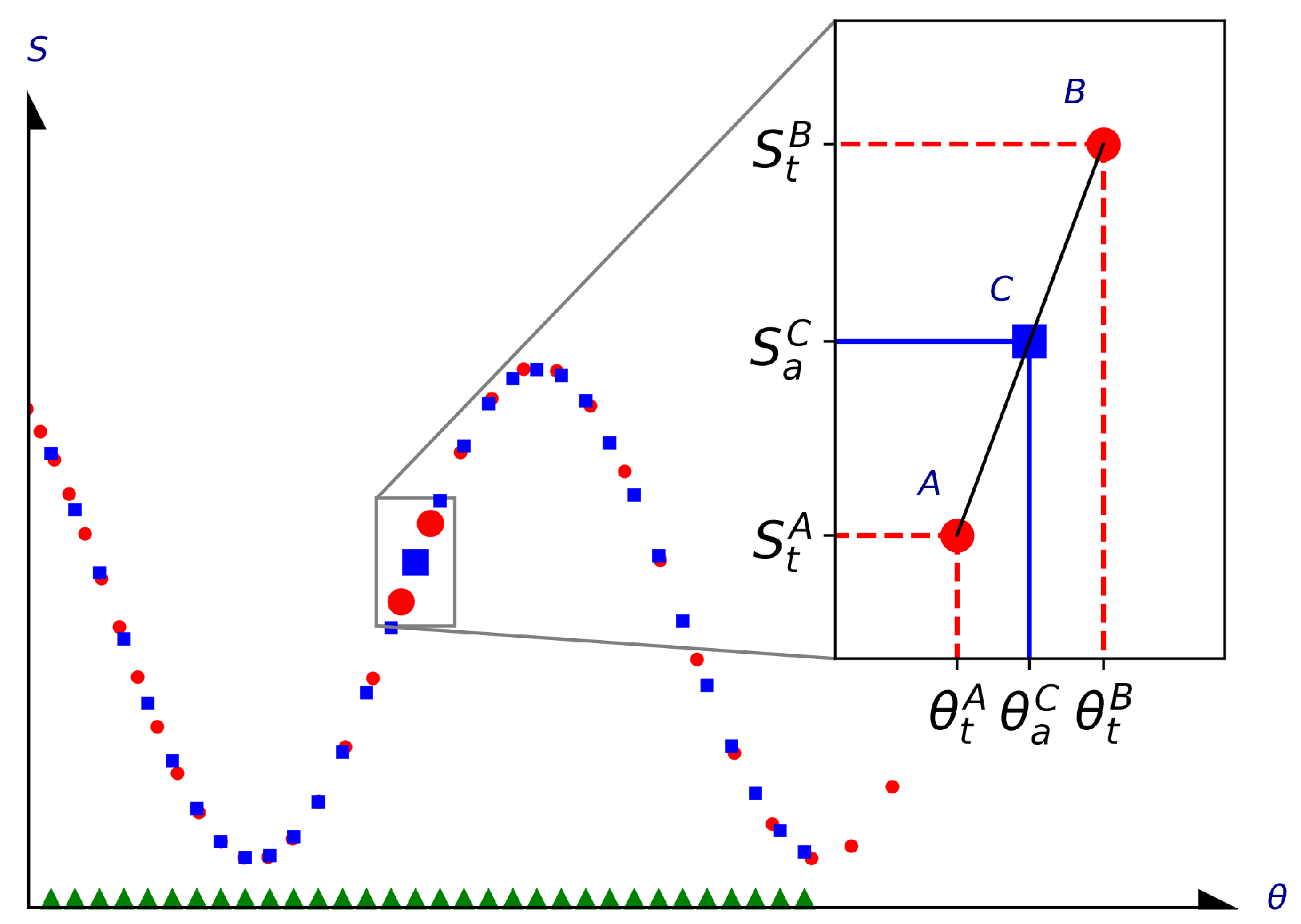
• The subscript “t” is used to indicate the series in the time domain. The time domain series is sampled at a constant sampling-rate with equal time intervals. They are basically non-stationary signals, which need to be resampled into the series with equal angular intervals. The rotor position angle series $\left\{{\theta }_t\left(t\right)\right\}$ and the non-stationary load torque signal series $\left\{S_t\left(t\right)\right\}$ are constructed using ${\theta }_{comp}$ and ${\widehat{T}}_L^{AC}$, respectively.
• The subscript “a” is used to indicate the series in the angular domain. An angular domain series $\left\{{\theta }_a\left(k\right)\right\}$ is created with equal angular intervals between each pair of adjacent points and drawn with “▲” markers in Figure 2

  $$\left\{{\theta }_a\left(k\right)\right\}=\frac{2\pi }{M}k,k=0,1,\dots ,N·M$$

  (15)

  where M denotes the sample number per revolution in the angular domain, which analogously resembles to the sampling frequency $f_s$ in the time domain. N represents the total number of revolutions in the angular domain, which, in the time domain, analogously resembles the time length of the series $T_{all}$.
• The load torque signal time domain series $\left\{S_t\left(t\right)\right\}$ is reallocated as the angular domain series $\left\{S_a^{{}^{\prime }}\left({\theta }_t\right)\right\}$, which is drawn in Figure 2 with “•” markers. $\left\{S_a^{{}^{\prime }}\left({\theta }_t\right)\right\}$ should be resampled at specific angular values listed in $\left\{{\theta }_a\left(k\right)\right\}$ to ensure an equal-angular-interval series in angular domain. As drawn in the zoom-in subplot of Figure 2, point $\mathbf{C}$ with “■” markers refers to an interpolation example point. Its horizontal ordinate is in series $\left\{{\theta }_a\left(k\right)\right\}$, and its vertical ordinate is calculated using linear interpolation

  $$S_a^C=S_t^A+\frac{S_t^B-S_t^A}{{\theta }_t^B-{\theta }_t^A}\left({\theta }_a^C-{\theta }_t^A\right)$$

  (16)

Similar to point $\mathbf{C}$, the Equation (16) will be implemented in sequence to all of the angular value within series $\left\{{\theta }_a\left(k\right)\right\}$, and all the interpolation points consist of the final result, the AR series $\left\{S_a\left(k\right)\right\}$ (the scatter with “■” markers in Figure 2).

After implementing angular resampling, the obtained series $\left\{S_a\left(k\right)\right\}$ becomes a stationary signal. The spectrum analysis can be applied for the purpose of BFD depending on the calculated order spectrum $P\left(o\right)$.

3.5. Fault Threshold Determination Using Information Entropy

To decide whether the amplitudes of the BFCOs are high enough in the calculated order spectrum $P\left(o\right)$ to indicate an existing fault, a threshold should be automatically adjusted according to the spectrum itself instead of being fixed to a preset value. A threshold generating algorithm is proposed in [36].

• Create two sliding windows, $w_A$ and $w_B$, whose lengths are $2L_A+1$ and $2L_B+1$ respectively.
• Move the sliding window $w_A$ through the whole $P\left(o\right)$, and calculate the average of the values included in $w_A$. A new order spectrum $P_a\left(o\right)$, called “average-value spectrum” can be obtained.
• Slide the window $w_B$ and calculate the median of the values included in $w_B$. A new order spectrum $P_d\left(o\right)$, called “median-value spectrum”, can be obtained.
• Calculate the maximum value $P_{max}$ of $P_d\left(o\right)$. It is defined as the threshold of the original spectrum $P\left(o\right)$.
• If the amplitude of $P\left(o\right)$ at the corresponding BFCO (or in its neighborhood) is higher than the $P_{max}$, it indicates that the motor is in a bearing fault condition and is in demand of the maintenance.

This method calculates the threshold basically based on the order spectra itself, and can effectively determine the fault threshold of the order spectra. Meanwhile, the lengths of the sliding window, $2L_A+1$ and $2L_B+1$, should be preset by researchers, and the different combinations of $L_A$ and $L_B$ will significantly influence the result of the threshold generation process.

In this paper, a window length determination algorithm is proposed to ease the influence introduced by the artificial parameter preset.

• Locate the impulses that are dominant in the order spectra by the method of information entropy $H_j$ described in [37].

  $$H_j=-\sum _{i=1}^j{p}_{i}log\left(p_i\right)$$

  (17)

  where $p_i$ represents the share of $P\left(i\right)$, the sorted values of the order spectra, in the sum of all $P\left(i\right)$ in the order spectra.

  $$p_i=\frac{P\left(i\right)}{{\sum }_{i=1}^{n}P\left(i\right)}$$

  (18)
  To decide whether the impulses are “dominant” in the order spectra, the differential of $H_j$ is calculated:

  $$H_j^{diff}=(H_j-H_{j-1})/H_j$$

  (19)
  If $H_j^{diff}$ becomes relatively small enough, all the $P\left(i\right)>P\left(j\right)$ should be regarded as “dominant impulses”.
• Calculate the weighted distances $D_i^{weighted}$ of the picked order spectrum value $P\left(i\right)$ using the following expression:

  $$D_i^{weighted}=\sum _j{d}_{ij}log\left[\frac{P\left(i\right)}{P\left(j\right)}\right]$$

  (20)

  where $d_{ij}$ indicates the distance between $P\left(i\right)$ and $P\left(j\right)$
• Among the $D_i^{weighted}$, the information entropy method is implemented again. If $H_{j-1}^{diff}\gg H_j^{diff}$ and $H_j^{diff}\approx 0$, $D_j^{weighted}$ will be set as $L_A$, the length of the average window.
• The length of the medium window, $L_B$, should be greater than $L_A$, and is set as $L_B=1.5L_A$.

Once the lengths of the sliding windows are determined by the algorithm listed above, the threshold of the order spectra can be calculated for bearing fault diagnosis.

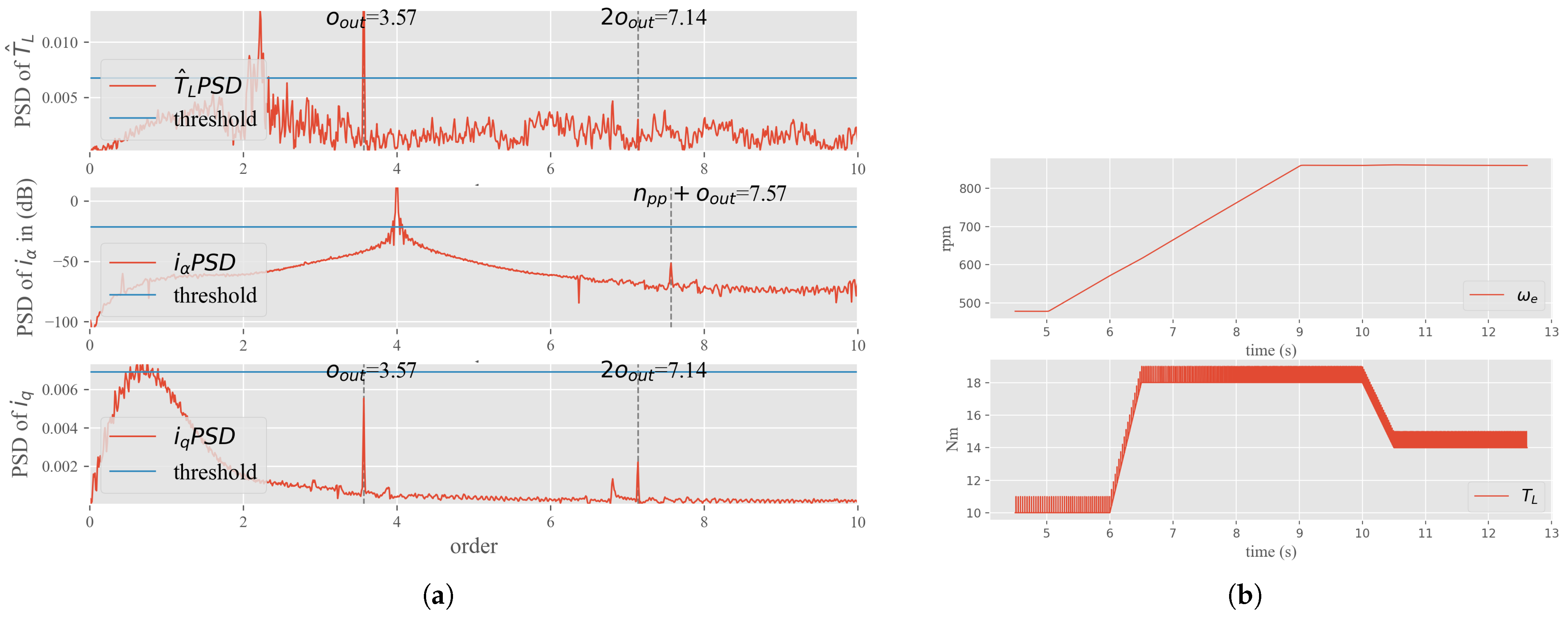
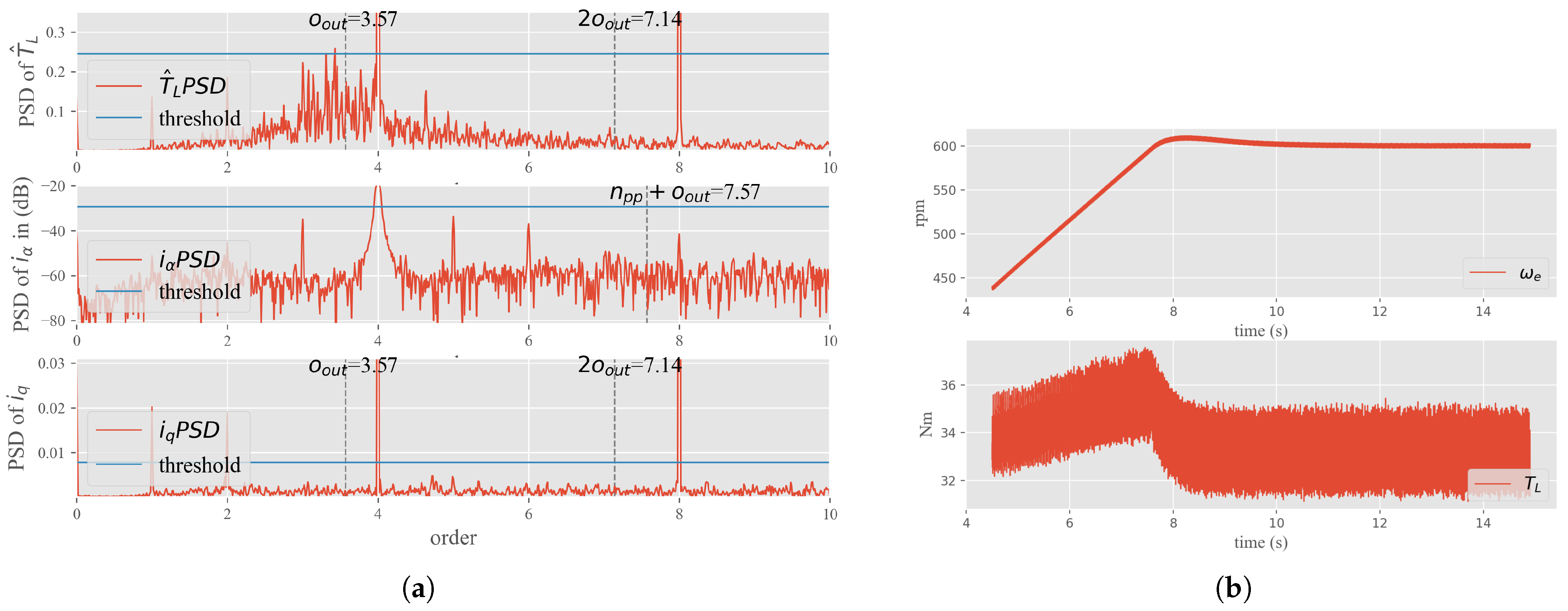
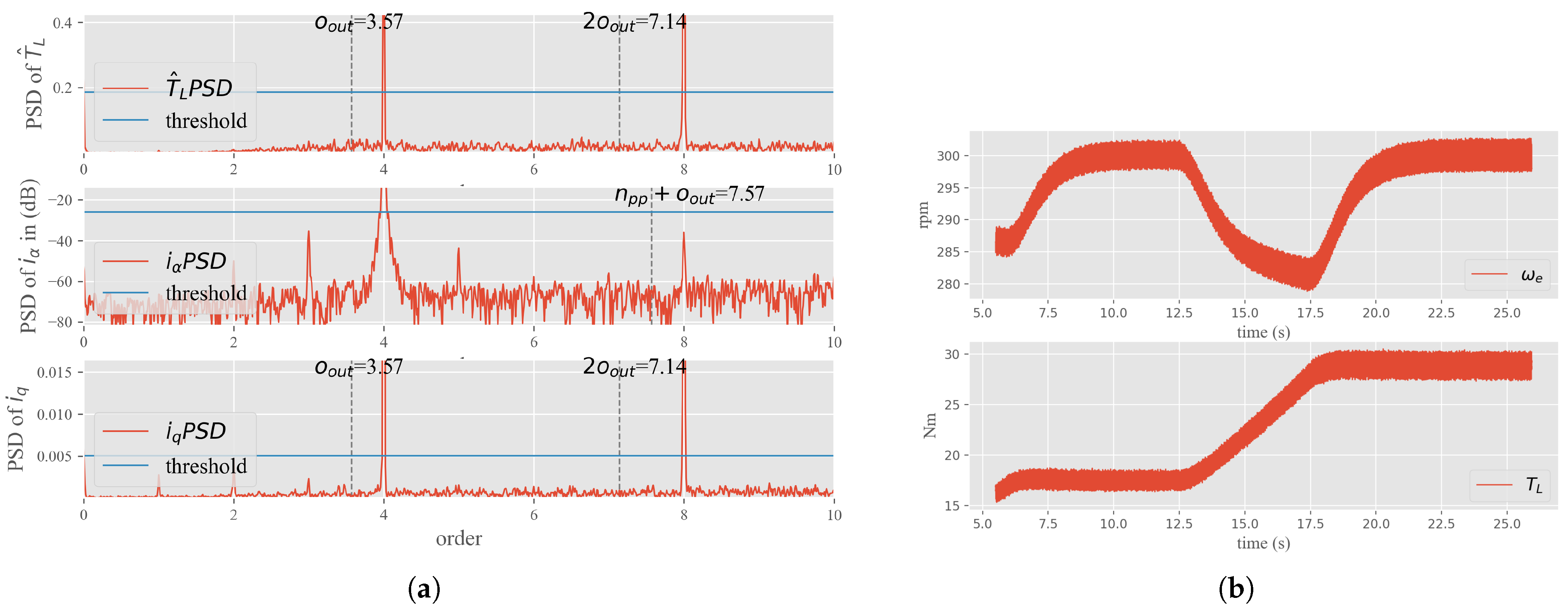
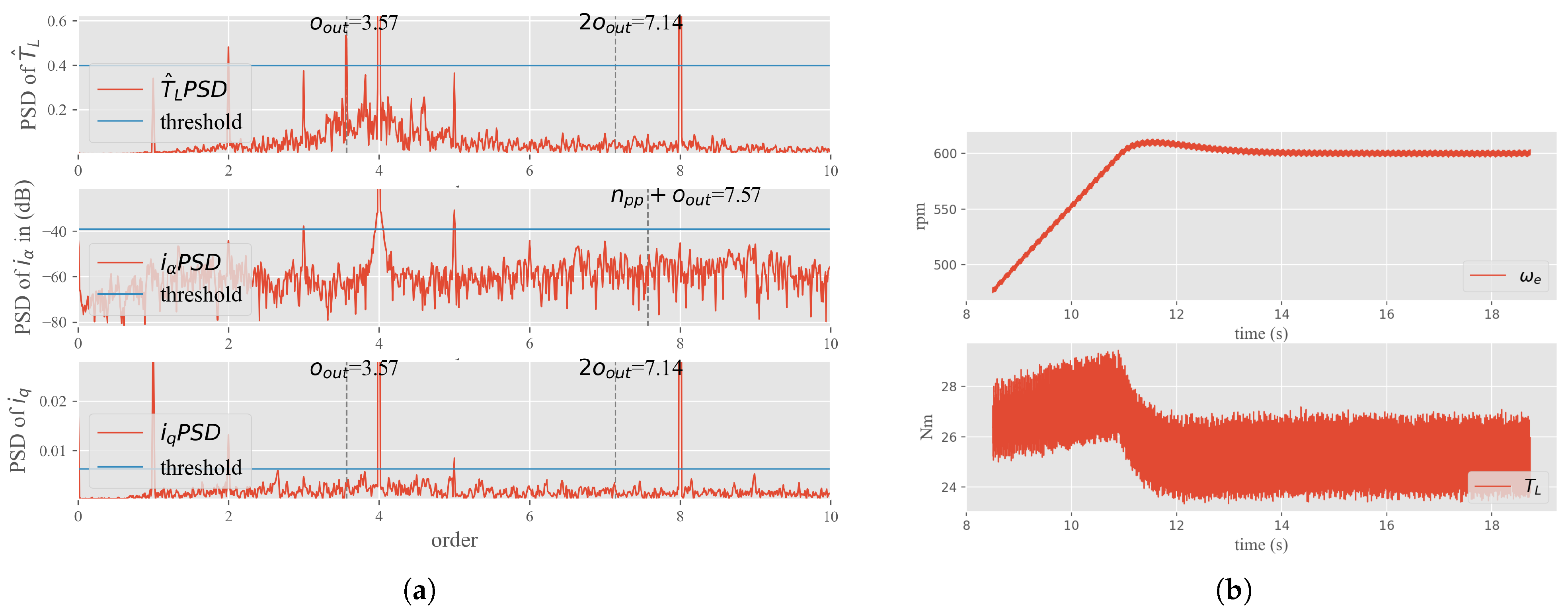
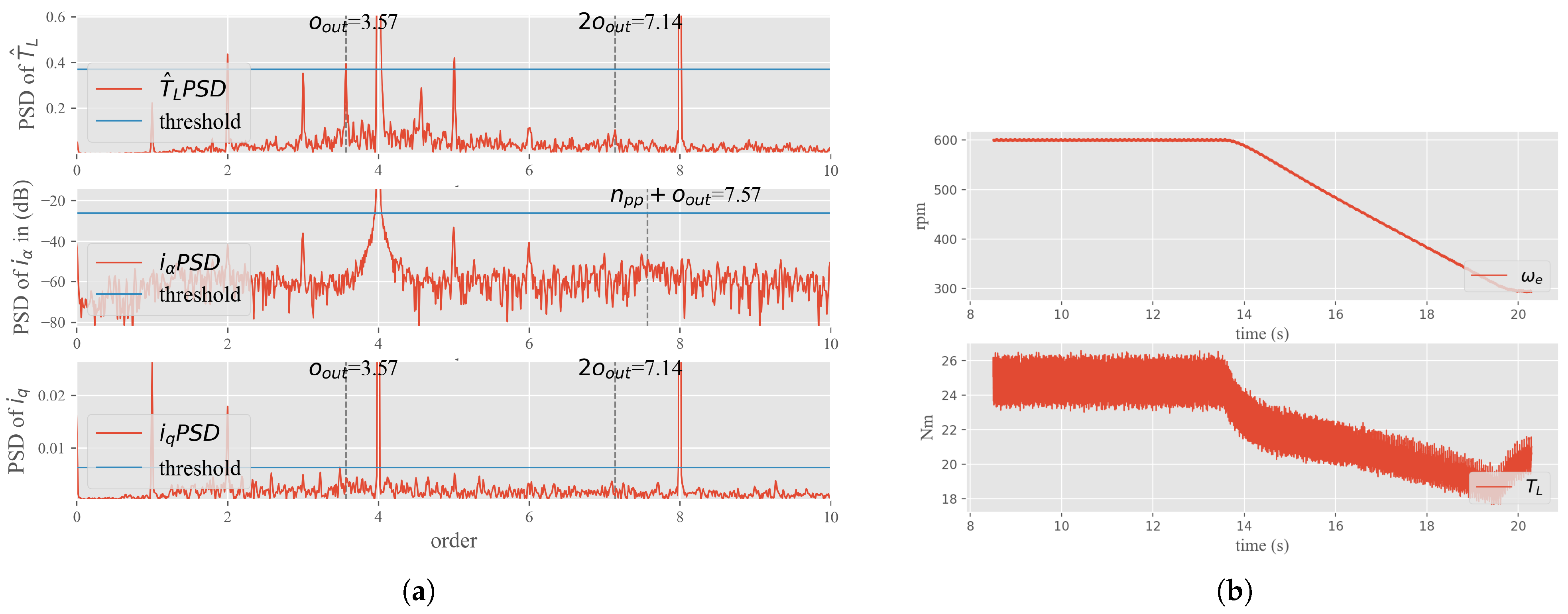
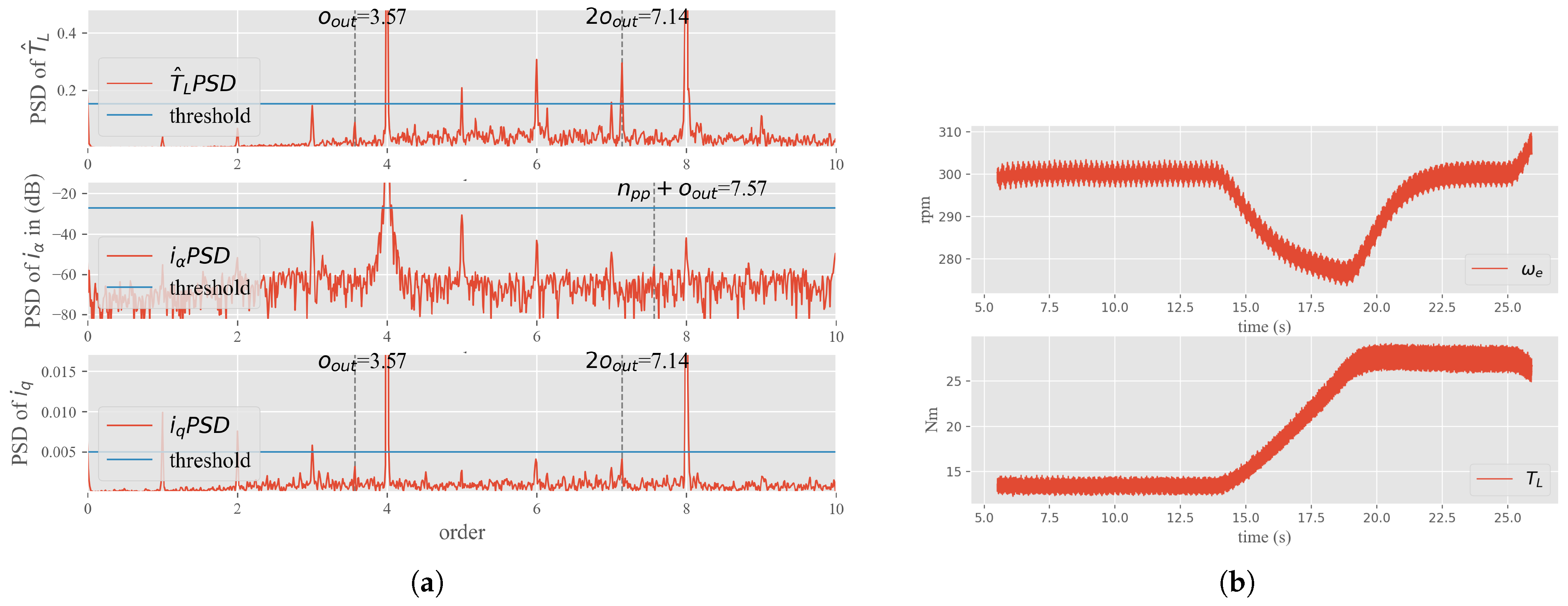
4. Simulation and Experimental Results

A rolling bearing was artificially damaged and reinstalled to the electrical motor for online experiment validation. Both speed varying and load torque varying experiments were conducted two times on the faulty bearing electrical motor. All six experiments, including the speed and load torque varying tests on the healthy bearing electrical motor, and one simulation result, on the condition that the speed and load torque varied simultaneously and background noises were added in the input currents and voltages, are compared with each other; the analyses are well discussed.

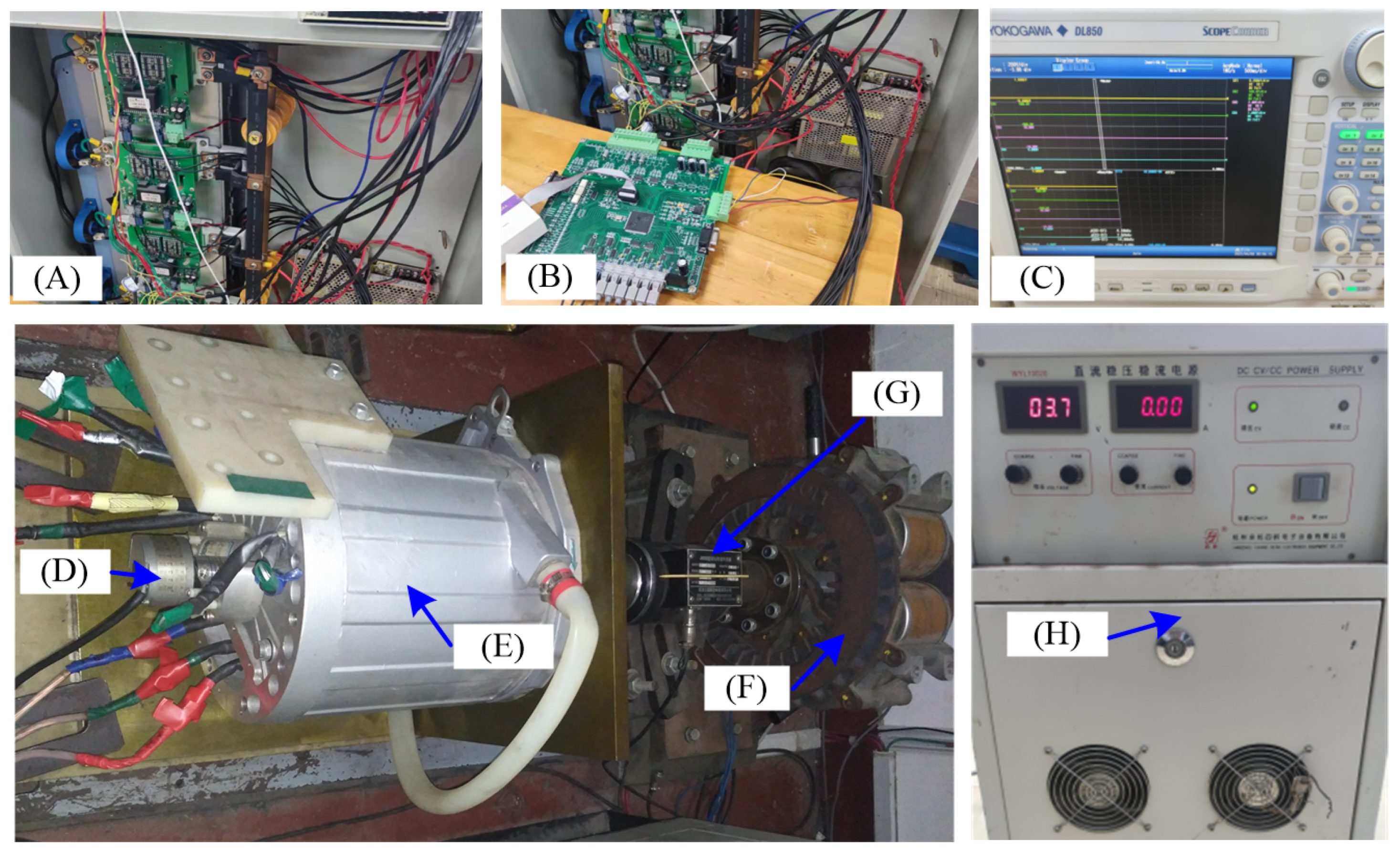
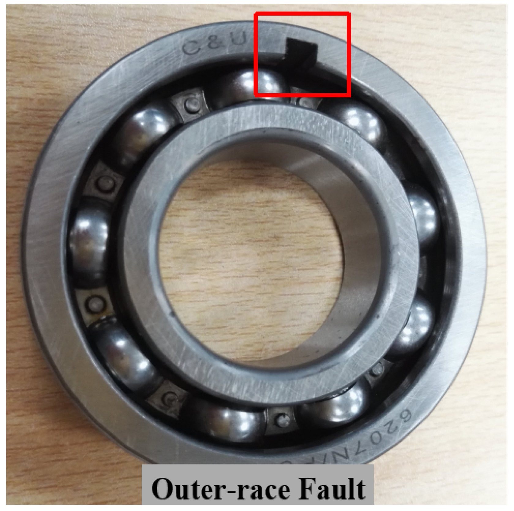
4.1. Experimental Setup

A 20 kW IPMSM is used as the test motor. Its parameters are listed in

Table 1. Parameters of the IPMSM. (Reprint with Permission [35]; 2018, Proceedings of the 2018 XIII International Conference on Electrical Machines (ICEM)).

Parameters	Notation	Values
Rated Power	$P_N$	20 kW
Number of Pole Pairs	$n_{pp}$	4
Stator Resistance	$R_s$	$0.021\Omega$
d-Axis Inductance	$L_d$	$0.59$ mH
q-Axis Inductance	$L_q$	$1.12$ mH
Rotor Flux	$\Psi$	$0.1$ Wb
Moment of Inertia	$J_m$	$0.28$$\mathrm{kg}·{\mathrm{m}}^2$

.

The motor is driven by an inverter that is controlled by a digital control board based on a 32-bit float-point 150 MHz TMS320F28335 digital signal processor. The voltage and current signals are recorded by a DL850E oscilloscope with voltage probes and current sensors, respectively, at a sample rate of 10 kHz. The resolutions of analog–digital converters in the oscilloscope for currents and voltages are both 12 bits. An electrodynamic eddy current brake was used as the load, supplied by a DC voltage source. The photographs of the aforementioned devices are shown in Figure 3.

The test bearing is SKF 6207-N. The geometric parameters are as follows: $N_b=$ 9, $\beta =$ 0, $D_p=$ 53.5 mm, and $D_b=$ 11 mm. The bearing is damaged artificially by wire-electrode cutting, as shown in Figure 4. A 5 mm-width slot is cut on the outer ring to emulate the outer raceway defect. According to (12), the bearing fault characteristic order of the bearing with the outer raceway defect $o_{out}$ is calculated as 3.57.

4.2. Simulation Results Using Natural Observer under Non-Stationary Conditions

A simulation was conducted using C language. The electrical motor model ran at the step-size of $5\times {10}^{-6}$ s. The step-sizes of the current loop and speed loop were $1\times {10}^{-4}$ s and $5\times {10}^{-3}$ s, respectively. The currents and voltages were added with uniform-disturbed noise with an amplitude of 0.02 before being imported into the observer. The outer raceway bearing fault was simulated by adding an impulse load torque signal with a constant angle interval, which was consist with the real BCFCs.

The non-stationary operating condition is drawn in the subplot (b) of Figure 5. As shown in the subplot, the varying period of speed and load torque overlapped, indicating that the motor was under rapid time-varying conditions. The order spectra of the estimated load torque ${\widehat{T}}_L$, the phase-$\alpha$ current $i_{\alpha }$, and q-axis current $i_q$ are listed. Compared with the order spectra of $i_{\alpha }$ and $i_q$, the peak at the BCFO $o_{out}=$ 3.57 exceeded the threshold in the order spectrum of ${\widehat{T}}_L$, while the other two order spectrums failed in the diagnosis. Further discussion that compares the simulation results with experimental results will be conducted in the following subsection.

4.3. Experimental Results Using the Natural Observer under Non-Stationary Conditions

Speed varying and torque varying experiments were performed for the faulty motor with the outer raceway defect bearing and the healthy motor.

The range of the speed command changed from 300 to 600 rpm. The acceleration and deceleration rate of the motor speed was set as 50 rpm/s. The load torque was set manually by tuning the output voltage of the DC voltage source shown in Figure 3, labeled as (H). The graphical transients of speed and torque are also represented in the subplots together with the order spectra of their corresponding operating conditions.

The estimated load torque ${\widehat{T}}_L$ was calculated by the natural observer, compensated, and angular resampled. The resample rate was 400 points per mechanical revolution and 40,000 points were used. As a result, the motor rotated 100 rounds in mechanical, in total, which means the resolution rate in the order spectrum equalled 1/100.

The phase-$\alpha$ current $i_{\alpha }$ and q-axis current $i_q$ were also resampled for comparison. The order spectrum of electrical quantity differed from the mechanical one due to the pair of poles $n_{pp}$ = 4, and the order resolution was adjusted to 1/100 in each order spectrum graph.

The healthy motor experiments results are shown in Figure 6 and Figure 7. In the case of the bearing fault motors, experiments under both speed/torque varying conditions were carried out two times, and all four experiment results are illustrated in Figure 8, Figure 9, Figure 10 and Figure 11, respectively.

In the order spectrum, the peaks located at integer orders represent the harmonics caused by the inevitable installation misalignment of the motor and load. In particular, order 4 was introduced by the fundamental component of the voltage and current since $n_{pp}=4$. These non-bearing-fault-related order components can be observed both in the healthy and faulty spectrum.

In the order spectrum of ${\widehat{T}}_L$ and $i_q$, the BFCO $o_{out}=$ 3.57 and its double order $2o_{out}=$ 7.14, are illustrated as gray dashed lines. In the case of $i_{\alpha }$, the BFCO should be $n_{pp}\ast (1+o_{out}/n_{pp})=$ 7.57, which is also drawn in the spectrum.

In the case of healthy motors, these peaks can hardly be observed at BFCOs in Figure 6 and Figure 7. Values at BFCOs are also under the threshold.

Two cases of speed time-varying condition experiments are illustrated in Figure 8 and Figure 9. Peaks at BFCO can be clearly observed in the order spectrum of ${\widehat{T}}_L$, the values also exceed the threshold. On the other hand, in the order spectra of $i_{\alpha }$ and $i_q$, values at BFCOs did not exceed the threshold, but were buried in the noise.

Another two cases of torque time-varying condition experiments are illustrated in Figure 8 and Figure 9. In the order spectrum of ${\widehat{T}}_L$, the peaks strongly indicate the existence of bearing fault at the double of BFCO, i.e., order 7.14. Peaks at BFCO are less obvious than order 7.14, but the threshold is also exceeded. Meanwhile, in the order spectrum of $i_q$, peaks can also be observed at BFCO and the double of BFCO. At last, a small peak at BFCO can be found in the order spectrum of the phase current $i_{\alpha }$(case1), but its value is under the threshold, which indicates that $i_{\alpha }$ is not capable for BFD under non-stationary conditions.

Compared with the simulation results, the order spectrums in the experiments differ in the following aspects. First, the peaks at integer orders induced by the inherent eccentricity of the motor shaft do not exist in the simulation order spectrums. Second, the amplitude of the low order (between order 0 and order 2) is higher in the simulation order spectrums than that of the experimental result. The reason could be the acceleration rate in the simulation is faster than experiments, resulting in the smearing phenomenon by the low order component.

To further demonstrate the advantages using the estimated load torque ${\widehat{T}}_L$ instead of the q-axis current signal, the signal-to-noise ratio (SNR) was calculated and compared. To calculate the SNR, order segment [0, 10] was selected from the whole order spectrum. The peaks located at the integer order, induced by the inherent eccentricity of the motor shaft, should not be considered in the SNR calculation. The peaks located at BFCO, 2*BFCO are regarded as signal power. All the values in the segment [0, 10] except those peaks are considered as “noise”. All four sets of faulty motor experiments were analyzed and SNR of ${\widehat{T}}_L$ and $i_q$ are calculated in

Table 2. The SNR of ${\widehat{T}}_L$ and $i_q$ in the faulty motor order spectra.

Motor Type	Faulty Motor
Time-Varying Condition	Speed (Case 1)	Speed (Case 2)	Torque (Case 1)	Torque (Case 2)
signal power of ${\widehat{T}}_L$	$5.60\times {10}^{-1}$	$2.65\times {10}^{-1}$	$1.77\times {10}^{-1}$	$1.39\times {10}^{-1}$
noise power of ${\widehat{T}}_L$	5.72	4.31	1.60	1.69
SNR of ${\widehat{T}}_L$	9.786%	6.140%	11.085%	8.226%
signal power of $i_q$	$3.36\times {10}^{-5}$	$2.27\times {10}^{-5}$	$2.20\times {10}^{-5}$	$4.22\times {10}^{-5}$
noise power of $i_q$	$4.91\times {10}^{-3}$	$4.60\times {10}^{-3}$	$9.12\times {10}^{-4}$	$1.68\times {10}^{-3}$
SNR of $i_q$	0.684%	0.494%	2.412%	2.509%

.

According to data in the Table 2, the SNR of ${\widehat{T}}_L$ is about 8.65 times of the SNR of $i_q$. The advantages using the estimated load torque ${\widehat{T}}_L$ instead of the q-axis current signal is then demonstrated.

Based on the experimental results, it is proven that the phase current and q-axis current signals are less effective compared with the estimated load torque signal in the BFD. The summary of the order spectra analysis results is listed in

Table 3. Summary of the order analysis results.

Motor Type	Healthy Motor		Faulty Motor
Time-Varying Condition	Speed	Torque	Speed (Case 1)	Speed (Case 2)	Torque (Case 1)	Torque (Case 2)
resampled ${\widehat{T}}_L$	×	×	√	√	√	√
resampled phase-$\alpha$ current	×	×	×	×	△	×
resampled q-axis current	×	×	×	×	△	△

Spectrum peaks at theoretical order: √: clearly observed; △: not obvious; ×: not observed.

.

5. Conclusions

This paper investigated the variations of load torque caused by the bearing faults in PMSM. The major contributions of this article include the following: a novel BFD method based on the natural observer for the PMSM is proposed. Bearing fault can be diagnosed under severe transient state working conditions without additional sensors, instead of steady-state working conditions, in which traditional diagnosis methods are required. The threshold generating algorithm makes the fault determination full-auto and decreases the occurrence of mistakes made by human-made decisions. The advantages of this estimated load torque ${\widehat{T}}_L$-based BFD were proven by experimental results, and the average ${\widehat{T}}_L$ SNR, which is about 8.65 times compared with the SNR of the traditional indicator $i_q$. The proposed method was proven to be more effective and reliable. Therefore, this method is applicable in the PMSM BFD under the non-stationary condition.

For future work regarding the propose method, some interesting problems still remain unsolved. The effectiveness of observer-based BFD on motors with different sizes and power need to be investigated for extending the application field of the proposed method. Time-varying conditions with highly random acceleration and deceleration should be validated by experiments for verification of the proposed method. An advanced demodulation method can be included in the framework to achieve a more precise diagnosis result.

References

1. Motor Reliability Working Group. Report of Large Motor Reliability Survey of Industrial and Commercial Installations. IEEE Trans. Ind. Appl. 1985, IA-21, 853–872. [Google Scholar] [CrossRef]
2. Tran, M.Q.; Elsisi, M.; Mahmoud, K.; Liu, M.K.; Lehtonen, M.; Darwish, M.M.F. Experimental Setup for Online Fault Diagnosis of Induction Machines via Promising IoT and Machine Learning: Towards Industry 4.0 Empowerment. IEEE Access 2021, 9, 115429–115441. [Google Scholar] [CrossRef]
3. Tran, M.Q.; Elsisi, M.; Liu, M.K.; Vu, V.Q.; Mahmoud, K.; Darwish, M.M.F.; Abdelaziz, A.Y.; Lehtonen, M. Reliable Deep Learning and IoT-Based Monitoring System for Secure Computer Numerical Control Machines Against Cyber-Attacks With Experimental Verification. IEEE Access 2022, 10, 23186–23197. [Google Scholar] [CrossRef]
4. Elsisi, M.; Tran, M.Q.; Mahmoud, K.; Mansour, D.E.A.; Lehtonen, M.; Darwish, M.M.F. Towards Secured Online Monitoring for Digitalized GIS Against Cyber-Attacks Based on IoT and Machine Learning. IEEE Access 2021, 9, 78415–78427. [Google Scholar] [CrossRef]
5. Elsisi, M.; Tran, M.; Mahmoud, K.; Mansour, D.E.A.; Lehtonen, M.; Darwish, M.M. Effective IoT-based deep learning platform for online fault diagnosis of power transformers against cyberattacks and data uncertainties. Measurement 2022, 190, 110686. [Google Scholar] [CrossRef]
6. Stack, J.R.; Habetler, T.G.; Harley, R.G. Fault classification and fault signature production for rolling element bearings in electric machines. IEEE Trans. Ind. Appl. 2004, 40, 735–739. [Google Scholar] [CrossRef]
7. Peeters, C.; Guillaume, P.; Helsen, J. A comparison of cepstral editing methods as signal pre-processing techniques for vibration-based bearing fault detection. Mech. Syst. Signal Process. 2017, 91, 354–381. [Google Scholar] [CrossRef]
8. Pezzani, C.M.; Bossio, J.M.; Castellino, A.M.; Bossio, G.R.; Angelo, C.H.D. A PLL-based resampling technique for vibration analysis in variable-speed wind turbines with PMSG: A bearing fault case. Mech. Syst. Signal Process. 2017, 85, 354–366. [Google Scholar] [CrossRef]
9. Teng, W.; Ding, X.; Zhang, Y.; Liu, Y.; Ma, Z.; Kusiak, A. Application of cyclic coherence function to bearing fault detection in a wind turbine generator under electromagnetic vibration. Mech. Syst. Signal Process. 2017, 87, 279–293. [Google Scholar] [CrossRef]
10. Schoen, R.R.; Habetler, T.G.; Kamran, F.; Bartfield, R.G. Motor bearing damage detection using stator current monitoring. IEEE Trans. Ind. Appl. 1995, 31, 1274–1279. [Google Scholar] [CrossRef]
11. Zhou, W.; Lu, B.; Habetler, T.G.; Harley, R.G. Incipient Bearing Fault Detection via Motor Stator Current Noise Cancellation Using Wiener Filter. IEEE Trans. Ind. Appl. 2009, 45, 1309–1317. [Google Scholar] [CrossRef]
12. Hamadache, M.; Lee, D.; Veluvolu, K.C. Rotor Speed-Based Bearing Fault Diagnosis (RSB-BFD) Under Variable Speed and Constant Load. IEEE Trans. Ind. Electron. 2015, 62, 6486–6495. [Google Scholar] [CrossRef]
13. Trajin, B.; Regnier, J.; Faucher, J. Comparison Between Stator Current and Estimated Mechanical Speed for the Detection of Bearing Wear in Asynchronous Drives. IEEE Trans. Ind. Electron. 2009, 56, 4700–4709. [Google Scholar] [CrossRef]
14. Phung, V.T.; Pacas, M. Detection of bearing faults in repetitive mechanical systems by identification of the load torque. In Proceedings of the 2016 IEEE 8th International Power Electronics and Motion Control Conference (IPEMC-ECCE Asia), Hefei, China, 22–26 May 2016; pp. 3089–3095. [Google Scholar] [CrossRef]
15. Bouchikhi, E.H.E.; Choqueuse, V.; Benbouzid, M.E.H. Current Frequency Spectral Subtraction and Its Contribution to Induction Machines’ Bearings Condition Monitoring. IEEE Trans. Energy Convers. 2013, 28, 135–144. [Google Scholar] [CrossRef] [Green Version]
16. Hu, C.Z.; Yang, Q.; Huang, M.Y.; Yan, W.J. Sparse component analysis-based under-determined blind source separation for bearing fault feature extraction in wind turbine gearbox. IET Renew. Power Gener. 2017, 11, 330–337. [Google Scholar] [CrossRef]
17. Escobar-Moreira, L.A. An approach to ultrasonic fault machinery monitoring by using the wigner-ville and choi-williams distributions. In Proceedings of the 2008 18th International Conference on Electrical Machines, Vilamoura, Portugal, 6–9 September 2008; pp. 1–6. [Google Scholar] [CrossRef]
18. Blodt, M.; Bonacci, D.; Regnier, J.; Chabert, M.; Faucher, J. On-Line Monitoring of Mechanical Faults in Variable-Speed Induction Motor Drives Using the Wigner Distribution. IEEE Trans. Ind. Electron. 2008, 55, 522–533. [Google Scholar] [CrossRef]
19. Seshadrinath, J.; Singh, B.; Panigrahi, B.K. Investigation of Vibration Signatures for Multiple Fault Diagnosis in Variable Frequency Drives Using Complex Wavelets. IEEE Trans. Power Electron. 2014, 29, 936–945. [Google Scholar] [CrossRef]
20. Watson, S.J.; Xiang, B.J.; Yang, W.; Tavner, P.J.; Crabtree, C.J. Condition Monitoring of the Power Output of Wind Turbine Generators Using Wavelets. IEEE Trans. Energy Convers. 2010, 25, 715–721. [Google Scholar] [CrossRef] [Green Version]
21. Eren, L.; Devaney, M.J. Bearing damage detection via wavelet packet decomposition of the stator current. IEEE Trans. Instrum. Meas. 2004, 53, 431–436. [Google Scholar] [CrossRef]
22. Lau, E.C.C.; Ngan, H.W. Detection of Motor Bearing Outer Raceway Defect by Wavelet Packet Transformed Motor Current Signature Analysis. IEEE Trans. Instrum. Meas. 2010, 59, 2683–2690. [Google Scholar] [CrossRef]
23. Li, Y.; Yang, Y.; Afshari, S.S.; Liang, X.; Chen, Z. Adaptive Cost Function Ridge Estimation for Rolling Bearing Fault Diagnosis Under Variable Speed Conditions. IEEE Trans. Instrum. Meas. 2022, 71, 1–12. [Google Scholar] [CrossRef]
24. Liu, Q.; Wang, Y.; Wang, X. Two-Step Adaptive Chirp Mode Decomposition for Time-Varying Bearing Fault Diagnosis. IEEE Trans. Instrum. Meas. 2021, 70, 1–10. [Google Scholar] [CrossRef]
25. Wang, J.; Peng, Y.; Qiao, W. Current-Aided Order Tracking of Vibration Signals for Bearing Fault Diagnosis of Direct-Drive Wind Turbines. IEEE Trans. Ind. Electron. 2016, 63, 6336–6346. [Google Scholar] [CrossRef]
26. Lu, S.; Guo, J.; He, Q.; Liu, F.; Liu, Y.; Zhao, J. A Novel Contactless Angular Resampling Method for Motor Bearing Fault Diagnosis Under Variable Speed. IEEE Trans. Instrum. Meas. 2016, 65, 2538–2550. [Google Scholar] [CrossRef]
27. Wang, T.; Liang, M.; Li, J.; Cheng, W. Rolling element bearing fault diagnosis via fault characteristic order (FCO) analysis. Mech. Syst. Signal Process. 2014, 45, 139–153. [Google Scholar] [CrossRef]
28. Bowes, S.; Sevinc, A.; Holliday, D. New natural observer applied to speed-sensorless DC servo and induction motors. IEEE Trans. Ind. Electron. 2004, 51, 1025–1032. [Google Scholar] [CrossRef]
29. Chen, Z.; Tomita, M.; Doki, S.; Okuma, S. An extended electromotive force model for sensorless control of interior permanent-magnet synchronous motors. IEEE Trans. Ind. Electron. 2003, 50, 288–295. [Google Scholar] [CrossRef]
30. Chen, J.; Mei, J.; Yuan, X.; Zuo, Y.; Lee, C.H.T. Natural Speed Observer for Nonsalient AC Motors. IEEE Trans. Power Electron. 2022, 37, 14–20. [Google Scholar] [CrossRef]
31. Ali, M.N.; Soliman, M.; Mahmoud, K.; Guerrero, J.M.; Lehtonen, M.; Darwish, M.M.F. Resilient Design of Robust Multi-Objectives PID Controllers for Automatic Voltage Regulators: D-Decomposition Approach. IEEE Access 2021, 9, 106589–106605. [Google Scholar] [CrossRef]
32. Zhao, L.; Huang, J.; Liu, H.; Li, B.; Kong, W. Second-Order Sliding-Mode Observer With Online Parameter Identification for Sensorless Induction Motor Drives. IEEE Trans. Ind. Electron. 2014, 61, 5280–5289. [Google Scholar] [CrossRef]
33. Li, B.; Chow, M.Y.; Tipsuwan, Y.; Hung, J.C. Neural-network-based motor rolling bearing fault diagnosis. IEEE Trans. Ind. Electron. 2000, 47, 1060–1069. [Google Scholar] [CrossRef] [Green Version]
34. Fyfe, K.; Munck, E. Analysis of Computed Order Tracking. Mech. Syst. Signal Process. 1997, 11, 187–205. [Google Scholar] [CrossRef]
35. Ye, M.; Huang, J. Bearing Fault Diagnosis Under Time-Varying Speed and Load Conditions via Speed Sensorless Algorithm and Angular Resample. In Proceedings of the 2018 XIII International Conference on Electrical Machines (ICEM), Alexandroupoli, Greece, 3–6 September 2018; pp. 1775–1781. [Google Scholar] [CrossRef]
36. Gong, X.; Qiao, W. Current-Based Mechanical Fault Detection for Direct-Drive Wind Turbines via Synchronous Sampling and Impulse Detection. IEEE Trans. Ind. Electron. 2015, 62, 1693–1702. [Google Scholar] [CrossRef]
37. Romero-Troncoso, R.J.; Saucedo-Gallaga, R.; Cabal-Yepez, E.; Garcia-Perez, A.; Osornio-Rios, R.A.; Alvarez-Salas, R.; Miranda-Vidales, H.; Huber, N. FPGA-Based Online Detection of Multiple Combined Faults in Induction Motors Through Information Entropy and Fuzzy Inference. IEEE Trans. Ind. Electron. 2011, 58, 5263–5270. [Google Scholar] [CrossRef]
Figure 1. Implementation of the proposed method.
Energies 15 03532 g001
Figure 2. Example of Angular Resample.
Energies 15 03532 g002
Figure 3. Experimental setup: (A) inverter, (B) control board, (C) oscilloscope, (D) encoder, (E) IPMSM, (F) brake, (G) torque transducer, (H) DC voltage source.
Energies 15 03532 g003
Figure 4. Test bearing with the outer raceway fault.
Energies 15 03532 g004
Figure 5. Simulation of the faulty motor (a) power spectrum density (b) graphical transients of speed and torque.
Energies 15 03532 g005
Figure 6. Speed varying experiment of the healthy motor (a) power spectrum density and (b) graphical transients of speed and torque.
Energies 15 03532 g006
Figure 7. Torque varying experiment of the healthy motor (a) power spectrum density and (b) graphical transients of speed and torque.
Energies 15 03532 g007
Figure 8. Speed varying experiments (Case1) of the bearing fault motor (a) power spectrum density and (b) graphical transients of speed and torque.
Energies 15 03532 g008
Figure 9. Speed varying experiments (Case2) of the bearing fault motor (a) power spectrum density and (b) graphical transients of speed and torque.
Energies 15 03532 g009
Figure 10. Torque varying experiments (Case1) of the bearing fault motor (a) power spectrum density and (b) graphical transients of speed and torque.
Energies 15 03532 g010
Figure 11. Torque varying experiments (Case2) of the bearing fault motor (a) power spectrum density and (b) graphical transients of speed and torque.
Energies 15 03532 g011