Abstract
Solid-state transformers (SSTs) are becoming an important solution to control active distribution systems. Their significant flexibility in comparison with traditional magnetic transformers is essential to ensure power quality and protection coordination at the distribution level in scenarios of large penetration of distributed energy resources such as renewables, electric vehicles and energy storage. However, the power electronic interface of SSTs decouples the nature of the inertial and frequency responses of distribution loads, deteriorating the frequency stability, especially under the integration of large-scale solar and wind power plants. Despite the virtual inertia/voltage sensitivity-based algorithms that have been proposed, the frequency sensitivity of loads and the capability of guaranteeing optimal control, considering the operating restrictions, have been overlooked. To counteract this specific issue, this work proposes a predictive control-driven approach to provide SSTs with frequency response actions by a strategy that harnesses the voltage and frequency sensibility of distribution loads and considers the limitations of voltage and frequency given by grid codes at distribution grids. In particular, the control strategy is centered in minimizing the NADIR of frequency transients. Numerical results are attained employing an empirically-validated model of the power system frequency dynamics and a dynamic model of distribution loads. Through proportional frequency control, the results of the proposed algorithm are contrasted. It is demonstrated that the NADIR improved about 0.1 Hz for 30% of SST penetration.
1. Introduction
The fast increase in variable generation has imposed challenging problems in power system operations. The low-to-zero inertia contribution of variable generation, its important variability, and its poor frequency responsiveness have eroded power systems’ robustness in terms of frequency stability [1,2]. As highlighted in [3,4], load contribution to inertial and frequency responses of the system is important and is overlooked because of the size of distribution loads, but it has been accounted for about 20% of the frequency response [5].
Load contribution to inertial and frequency responses can be limited if solid-state transformers (SSTs) are implemented in distribution feeders. SSTs are conceptually a power electronic-based transformer, which from a distribution feeder point of view, provide several advantages compared to a standard passive transformer, such as: high power density, active power factor correction, controlled bidirectional power-flow, voltage and frequency regulation, active filtering, disturbance isolation, direct interconnection of different frequency systems and the access to an LV DC-link [6,7].
However, the SSTs operation results in the decoupling of the influence of power system voltage and frequency on distribution loads. In power grids with traditional magnetic transformers, the voltage and frequency dynamics are reflected in loads, achieving inertial and frequency responses that contribute to frequency stability. Meanwhile, by incorporating a certain number of SSTs to the power grid, the supplied voltage and frequency to loads are independent of those of the grid, preventing the occurrence of the inertial and frequency responses. Thus, the SSTs’ integration, in principle, deteriorates the power system frequency stability.
The aforementioned issues have been addressed in the literature by proposing synthetic methods for supporting the frequency stability via SSTs. For instance, a hybrid transformer with the capability of emulating virtual inertia is proposed in [8]; meanwhile in [9], a method to support the primary frequency control by configuring the SST as a virtual synchronous machine (VSM) is proposed. Both works introduce algorithms to release the stored energy available at the DC-link of the back-to-back (B2B) converter, so they do not take advantage of the dynamic responsiveness of loads. Other approaches to deal with those problems are introduced in [10,11], where the authors present the support for the primary frequency control by regulating the voltage-sensitive loads connected to the SST. Another research tackling this issue presents a combination of virtual inertia and voltage-sensitive load-based droop controllers applied over a hybrid AC/DC network [12]. However, the common factor for all previous proposals is to model the limitations of voltage and frequency presented in grid codes by considering saturation effects, which are not explicitly represented as constraints on the control algorithms, and by overlooking stability issues well-described in the literature [13]. In addition, the performance of the control action is not taken into account since the optimal criteria of control actions are not analyzed.
In contrast with the state-of-the-art, this paper proposes a predictive control-based, frequency-responsive algorithm for SSTs focused on minimizing the magnitude of NADIR, which is defined as the lowest point during a frequency excursion. Minimizing NADIR is a key step in avoiding the triggering of under-frequency load shedding under massive penetration of renewable energies [14]. This is carried out by the voltage and frequency regulation that SSTs provide to loads and can be defined as a control rule. In addition, the control algorithm explicitly includes constraints to prevent grid code violations of voltage and frequency, ensuring its compliance for any operating condition.
Thus, the highlights of the proposed predictive control-based frequency-responsive algorithm can be summarized as follows:
- The algorithm minimizes the Nadir magnitude.
- The optimal solution considers the operational constraints regarding the tolerance band of frequency and voltage.
- The frequency-sensitivity of loads is included in order to improve the load contribution.
The proposed strategy is numerically evaluated using an empirically-validated model and a reduced-order model that represents the power system frequency dynamics, together with a dynamic model for all loads.
2. Dynamic Models
2.1. Frequency Response
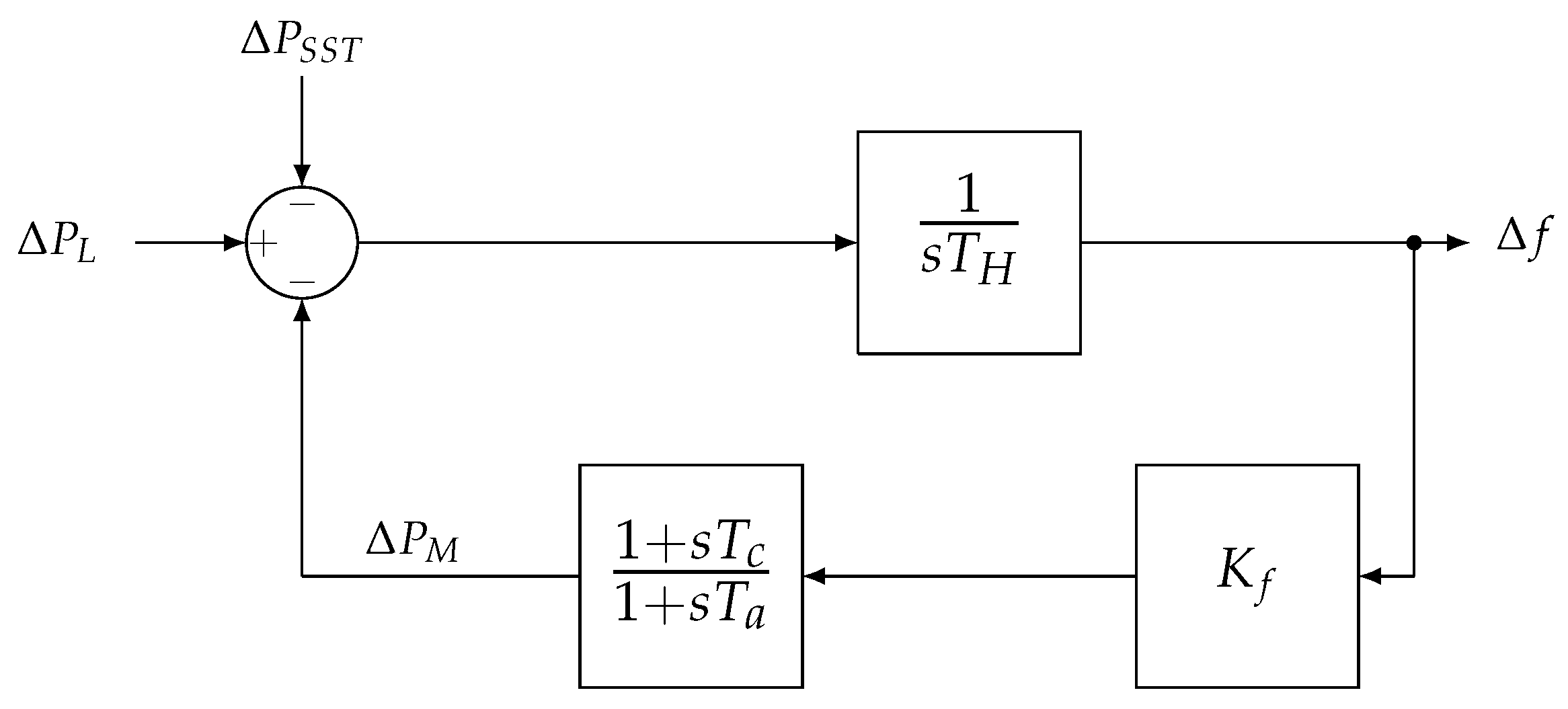
In general, frequency studies for advance control purposes consider dynamic equivalents derived from high-order power system models; this work particularly considers the model presented in [15]. By means of synchrophasor data recorded after generation contingencies occur, a system identification technique is used to gain a reduced-order model that represents an actual frequency behavior of a power system. One modification to the original model is the addition of a power input , which is associated with the contribution of SSTs. The model is shown in Figure 1.
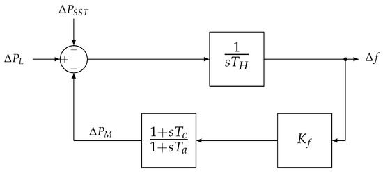
Figure 1.
Simplified model for the frequency dynamics adapted. Reproduced from [15], IEEE: 2012.
whose state-space representation is shown in (1):
where the changes in the state vector are denoted by and the state matrix is symbolized as , and the input matrix is defined as , such that
where,
- : system frequency deviation (Hz),
- : system governors power response (MW),
- : system power imbalance (MW),
- : system inertia (MWs/Hz),
- : frequency response from SST (MW),
- : model dynamic parameter (s), and
- : governor droop of the system (MW/Hz).
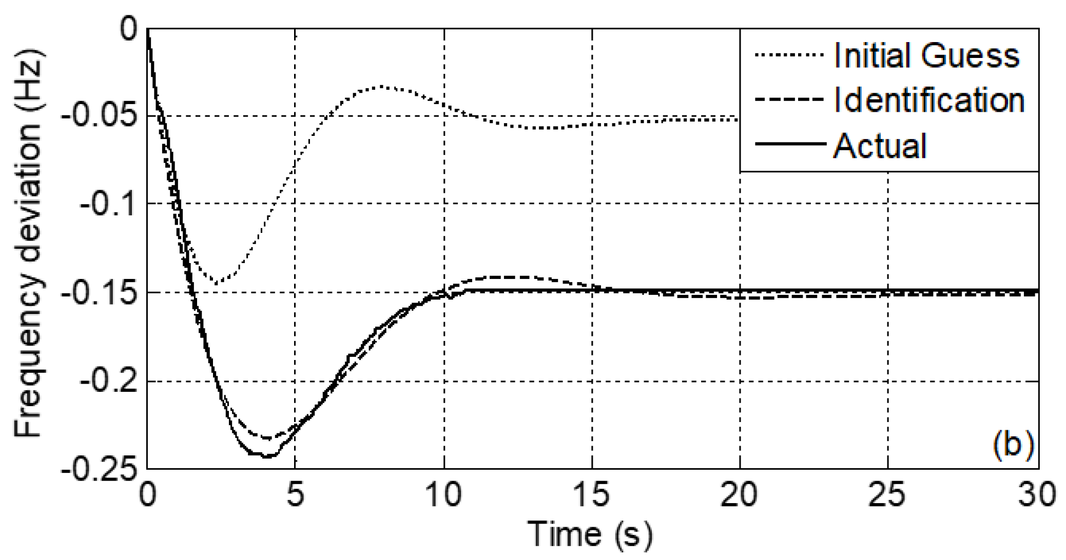
The parameters of the model were identified with actual frequency behavior in [15]. A frequency event in the Electric Reliability Council of Texas (ERCOT) in 26 January 2010 at 1:58 am was considered to perform an identification process to obtain the result in Figure 2 and the set of parameters in Table 1.
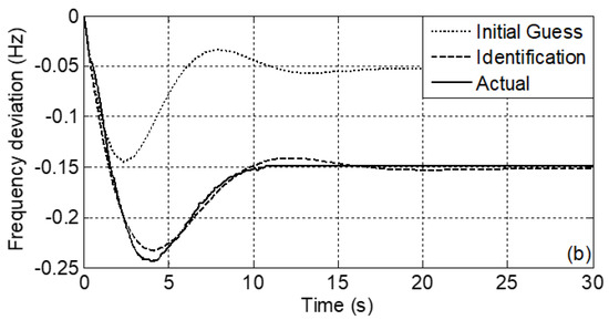
Figure 2.
Comparison between the actual and identified systems. Reproduced from [15], IEEE: 2012.

Table 1.
Conditions and parameters for performing the system identification. Reproduced from [15], IEEE: 2012.
Thus, a reduced-order and empirically-validated model that represents frequency dynamics is considered. Since this model does not differentiate the contribution of synchronous load from total inertia and frequency response, this fact is addressed in the following sections. Note that is meant to model the load response through an SST, which is different from the natural response of the loads that remain connected through magnetic transformers. This is also modeled in the following sections.
2.2. Load Dynamics
The load model has three cases to be modeled:
- Load is connected through a traditional transformer, maintaining its current dynamic bond with the power system,
- Load is connected through an SST with no particular control, so all load frequency response is suppressed, and
- Load is connected through an SST with dedicated frequency control, so load will present some response to power system frequency.
An initial step is to represent the load contribution to inertial and frequency responses in model (1) associated with loads synchronously connected through magnetic transformers.
2.2.1. Synchronously Connected Demand
As shown in model (1), represents the system’s overall synchronous inertia, including loads and generators. The load inertia is expressed in terms of a percentage of total system inertia , and the demand frequency response is normally measured with a frequency droop that depends on the amount of load. For instance, it is estimated in the UK that demand supplies about 20% of the system inertia [5] and varies by 2.5% per Hertz [16]. Aiming to model load inertia and frequency response, proportional models are proposed, as shown in (2) and (3), considering the values of Table 1.
where and are the load contributions to inertia and frequency response, respectively. Note that these numerical values are relative to the identified event in Figure 2 and Table 1.
Intuitively, both contributions are reduced as the integration of SSTs increases due to the dynamics decoupling (assuming no frequency control for SST). As a simplified assumption, this paper considers that demand response changes proportional to the per unit integration of SSTs, namely , as shown in Equations (2) and (3).
= 1 indicates that all feeders are implemented with SSTs, so = 0 (no inertial response from loads). = 0 indicates that no feeder is implemented with SSTs, so = 1226 (no change from the base case in Figure 2). In this context, the total inertia and droop shown in Table 1 must be adapted in order to consider the electromagnetic decoupling produced by the SSTs. Thus, the total inertia and droop become:
This model overlooks the diverse nature of distribution feeders that can be industrial, residential, commercial or a combination of them. In this sense, the integration of SSTs can replace feeders of a particular nature, so the influence of that integration into the overall behavior may not be linear. Thus, an accurate modeling of those aspects is left for future work.
2.2.2. Synchronous Demand Connected through SST
As stated in (6) and (7), is used to model the penetration level of SSTs for the case when no synthetic frequency control is considered. Thereby, the SST-interfaced demand, as mentioned above, cannot contribute naturally to frequency response due to the absence of an electromagnetic coupling with the power system. Since there are synthetic methods to support the frequency regulation from the SST-interfaced demand, a dynamic model of loads is still necessary to assess the demand response due to SSTs supply frequency and voltage, which in turn can be managed to obtain a desired behavior.
Despite the fact that several representations have been proposed, at the present time there is no dynamic load standard model [17]. Nevertheless, as a load seen from a distribution feeder is a combination of different static and dynamic devices, a model that combines both components is usually considered. This model is known as a composite load model.
In this paper, the constant impedance (Z), constant current (I), constant power (P), and ZIP-Induction motor load model presented in [18] are used to represent the response of loads connected through SSTs, where static and dynamic components are described by a ZIP model (8) and third-order induction motor equivalent model in the rotor current reference frame (9), respectively.
where the variables and stand for the direct and quadrature components of the SST supplied voltage, and correspond the direct and quadrature components of load current, denotes the equivalent motor speed, and represents the frequency supplied by the SST. Meanwhile, symbolizes the overall active power response of the modeled load, and the set of parameters , , , , , H, , , , , , and are described in Table 2, whose values are obtained in [18] through online measurement data and identification in a 131/69 KV load substation in the Taiwan power system.
Table 2.
Composite load model parameters. Reproduced from [18], IEEE: 2006.
To simplify the demand response analysis, a linearized version of (9) over the operational point shown in Table 2 is described in (10).
where ,, , , and are respectively expressed by:
Then, the per unit load dynamic behavior can be represented for frequency control studies with the SSTs’ integration.
2.3. Solid-State Transformer Model
This modeling is founded on the principles of the composite load model presented above, since a synthetic response of the demand connected to SSTs may be obtained by controlling the frequency and voltage output ( and of the SST in (10). It is noteworthy that the control variables , and can be set freely as parameters of the SST, so the control action is, in principle, independent of the dynamics of the B2B converter of the SST.
Since B2B power electronic converters normally rely on the DC link capacitor bank voltage to control the power balance of the energy conversion. The power balance takes advantage of the fact that, if the SST input power is greater than the power absorbed by load , the per unit voltage of the capacitor bank will increase, as shown in Figure 3.
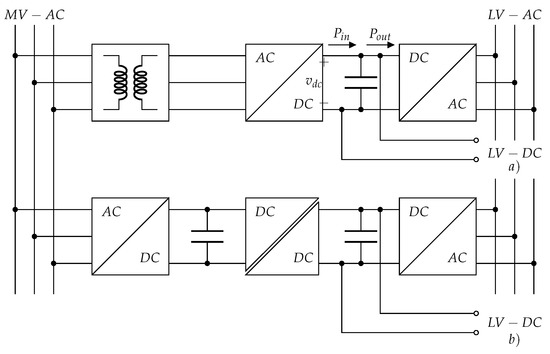
Figure 3.
Schematic diagram of (a) a passive transformer with a back-to-back rectifier/inverter stage; (b) SST.
For this study, a simple SST model consisting of a grid-side converter and a load-side converter [19] is presented in Figure 3b. More complex power electronics SST topologies, as depicted in Figure 3a, are left for future work. The DC-link power balance control regulates retaining a constant DC-link voltage, which is associated with the dynamic described by (11).
where C is the per unit capacitance of the DC link. It can be seen that the DC-link voltage change tends to zero only when the change of power also tends to zero. Normally, the rate of change of voltage is small, so can be assumed constant for (11) to be linear. To preserve the power balance, a proportional controller is used to manage the input power , aiming to match the power absorbed by the loads , as shown in Figure 4 (note that the plant to be controlled has a pole in the origin, so no integral control is needed). The tuning of the proportional controller gain was performed through a pole placement technique aiming to achieve a rising time of 0.01 seconds. The base quantities of C and were = 1000 F and = 400 Vdc, respectively, obtaining = 33.
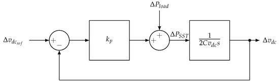
Figure 4.
DC-Link power balance control.
is implemented by the power electronics converter through the grid side converter in [20], where the rectifier’s active power transference is controlled by the rectifier direct component current, which involves other dynamics at the level of the electric transients. However, those dynamics are significantly faster than that of the frequency control under analysis in this work, so a detailed modeling of them is not necessary. will represent the per unit power consumption of loads connected to the SST. Thus, the state-space representation of the SST dynamics is shown in (12).
where,
In this work, the load model is assumed as a lumped-load model representation that groups the power system load dynamics. Thus, the total load is = 27,280 MW according to Figure 2 and Table 1. Since the load model in (10) has a per unit representation, it can be scaled up to represent physical units consistent with the study case.
Similar to the case of synchronous demand, the synthetic contribution of non-synchronous demand depends on the degree of integration of SSTs defined by . The SST-connected load contribution will consider the factor to determine the frequency control contribution and be proportional to the degree of integration . Then, (10) can be rewritten to represent the scaling factor and the SSTs’ penetration, as shown in (13).
Regarding the solid-state dynamics, the SST model embodies the collective response of a certain number of SSTs associated with a set of distribution feeders.
2.4. Power System Dynamic Model with Coupled Dynamics
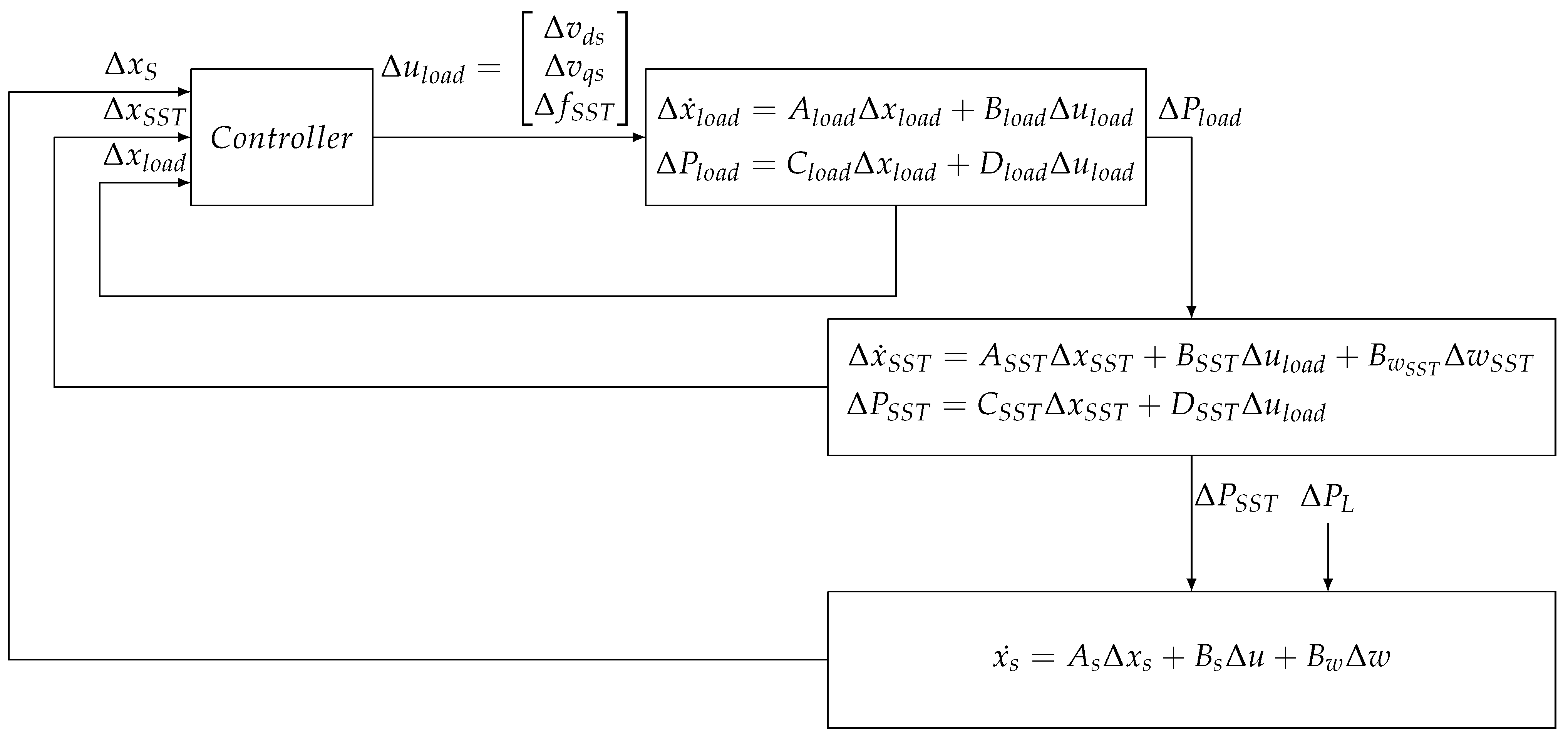
The interaction between SSTs’ dynamics, load dynamics and frequency dynamics leads to a set of coupled dynamics. It is possible to claim this fact since (1), (10) and (12) are linear systems that can be combined in a new linear system and can be interpreted as a block diagram, as shown in Figure 5.

The whole set of power system dynamics can be re-written as:
3. Control Proposal
A controller is proposed to regulate the power system dynamics associated with SSTs and loads in the scheme in Figure 5. It will set the SST voltage , and frequency to loads aiming to gain a power response to restore the load frequency response that is decoupled by the SST. To execute the control action, the controller will have access to the state variables of the system involved in the phenomena, which will allow considering an advance control technique. The control objectives have to consider the following features:
- Minimize the NADIR of the power system, particularly after large generator outages, over all feasible control actions;
- guarantee stability over all operating conditions; and
- guarantee that , and comply with the limits that distribution grid codes impose.
Among the advance control techniques that can address the needs described above, the continuous-time model predictive control (MPC) is formulated. In particular, the technique was chosen mainly because of its explicit way to include control action constraints, which is useful in this case to add the tolerance band of voltage and frequency. Other advanced stated-feedback control techniques, such as and , cannot easily integrate control action constraints that must be aggregated to the optimization program within the solvers, for example, via linear matrix inequalities. The MPC formulation allows a simple and direct integration of such constraints, which is the main reason why this particular technique was selected. Regarding a comparison with other studies, the paper compares the performance of the proposed algorithm with a proportional controller. As no other similar techniques for this application were found in the state-of-the-art, a proportional control was the closest control technique to perform a comparison.
3.1. Continuous-Time Model Predictive Control
The MPC is an algorithm that computes the trajectory of the control action for the output state to remain as close as possible to a desired reference, and it also optimizes metrics of the state variables and the control actions. Among all techniques available in the state-of-the-art, the continuous MPC using orthonormal functions proposed in [21,22] is chosen to prevent the discretization of the state-space model with coupled dynamics in (14). The algorithm is based on the principle that any arbitrary function , that satisfies the condition (15) can be approximated by using a finite set of orthonormal functions (16), where , are coefficients , are orthonormal functions and k is the number of orthonormal functions used.
Considering the system (14) under analysis, the control action does not conceptually fulfill condition (15) since the expected control action is supposed to obtain some droop control from loads, which represents a sustained control action in the time scale of primary control. Then, this sustained control action does not comply with this condition. To address this difficulty, the control definition will consider the derivative of the control action . To guarantee stability, the control action will reach steady-state within the time scale under analysis, so the derivative of the control action will tend to zero, fulfilling condition (15). Thus, the derivative of the control signal is described by the orthonormal functions (17).
3.1.1. Laguerre Representation of the Control Actions
Despite the fact that there are several types of orthonormal functions that satisfy the condition (18), the literature recommends the use of two of them: Laguerre or Kautz functions [21,22].
This paper considers the use of Laguerre functions as they have the advantage of requiring the tuning of only one time scaling factor parameter p, which corresponds to the pole of the Laguerre functions. The literature [21] indicates that this parameter should be tuned until an adequate dynamic response is obtained.
Let be the Laguerre functions vector and the coefficient vector; using these definitions, (17) becomes (20). In addition, it is shown that a representation of the Laguerre functions vector can be obtained in (21), assuming the initial condition of the Laguerre functions vector.
Thus, three control signals , and can be represented by their Laguerre equivalents.
3.1.2. Representation of Disturbance Derivative in the Continuous MPC Formulation
Note that the first derivative of the control signal does not appear explicitly in (14), so an augmented state-space model is required. This is obtained through using auxiliary variables as follows:
Then, one can define a new state variable vector for the augmented state-space model is derived in (23). Notice that this model employs the first derivative as an input, whereas the output is the same as model (14).
If the state vector is available at the current time . Then at the future time , > 0, the predictive state variable can be obtained by using the derivative of the signal control computed in (17). The resulting equation is shown in (24). It is noteworthy that the predictive state variable must be computed at each sampling interval until the predictive horizon is completely covered.
Once the predictive state variable is computed, the optimal control signal is determined by minimizing the objective function defined in (27), where denotes the future desire reference and stands for the predicted output state defined in (28). Matrices Q and R are weighted matrices of the predictive state output and the control signals, respectively.
By introducing (20) in (27), then (29) is obtained. By taking advantage the orthonormal property of the Laguerre functions defined in (18), (29) results in (30)
Finally, defining (34)–(36), (33) becomes (37). Thus, the problem of minimizing the objective function defined in (27) is essentially a quadratic programming problem, where the decision variable is . In this context, the problem can be algebraically solved to obtain a constant control law in absence of any constrain. However, if constraints are added to the problem (27), then the optimization problem must be numerically solved for each predictive step .
In the particular case of this application, the control action must be constrained, complying with grid code requirements. For instance, the National Grid Power System (UK) establishes that the operational system frequency must be within a ±1 Hz around the scheduled value [14] and the supplied voltage must be within a band of ± of its nominal value [23]. Assuming that the low voltage-bus of the SST is roughly balanced, the resulting q-component when the original Park and Clark transforms are applied is zero. Then, the following constraints are added to (37).
Note that the control signal constraints must be expressed as function of the decision variables in order to solve the quadratic programming problem (37). This can be computed through (39), where is the sampling time and is defined by (40)
Finally, the weighted matrices Q and R indicate the relevancy of the states and control variables for the algorithm. In the case of the state variables, the objective is just centered in minimizing the NADIR, thus matrix Q has just one coefficient different from zero related to this variable (43). With respect to matrix R, it has to be positive semi-definite, a particular value that showed satisfactory simulation results is enclosed in (43).
4. Simulation
4.1. Study Case
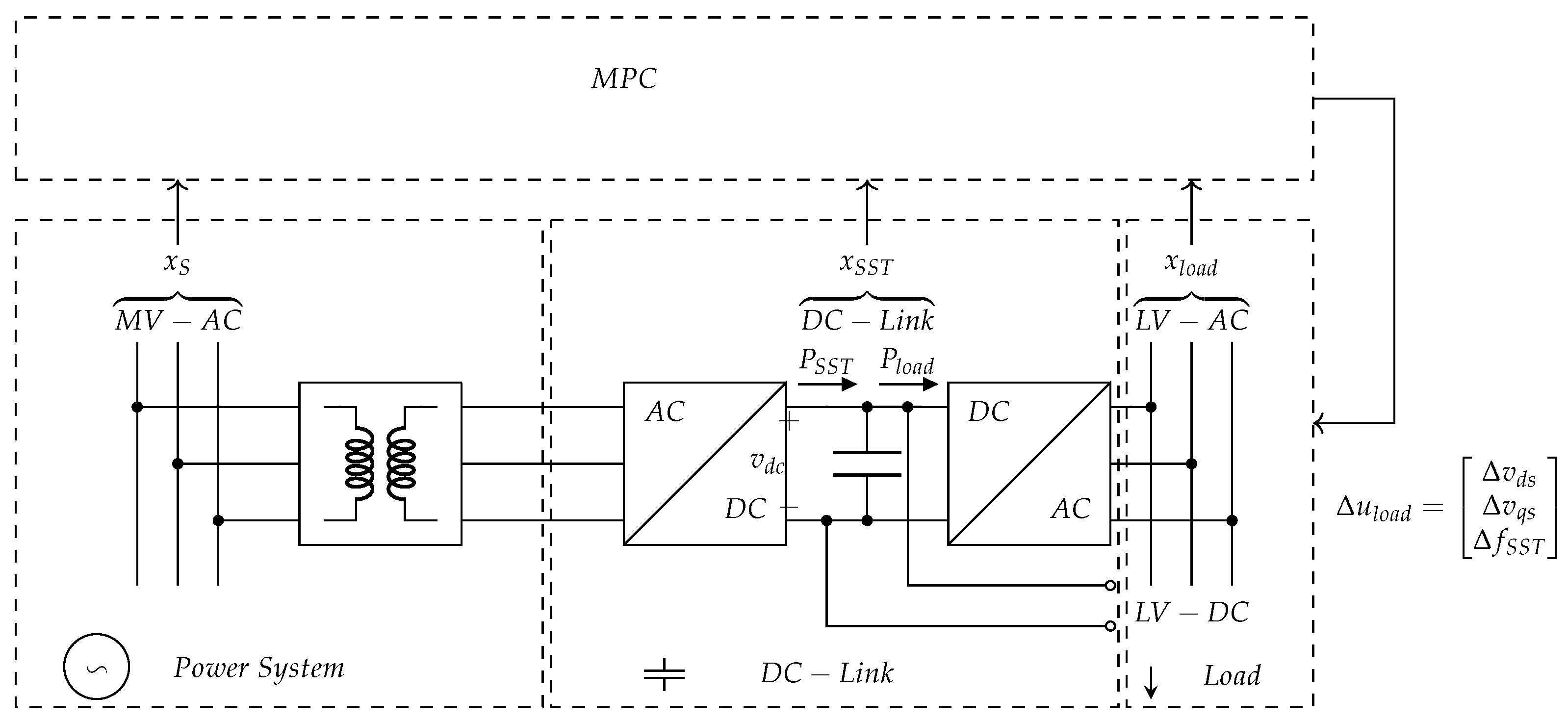
Aiming to assess the performance of the proposed continuous MPC-frequency feedback control depicted in Figure 6, a sudden disconnection of 2000 MW in the power system is considered. This contingency was associated to the trip of a large nuclear power plant.
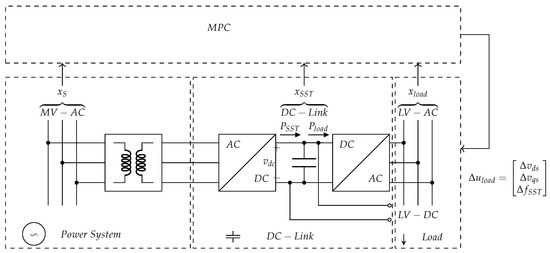
Figure 6.
Circuit diagram for the implementation proposed predictive control-based frequency-responsive algorithm.
To evaluate the performance of the proposed control, the proposed control algorithm will be compared with a simpler proportional control, as the one proposed in [24]. The idea behind this comparison is to only feedback the frequency signal and to ensure that the grid code’s limits are not violated for the extreme conditions. Let , , and be the maximum and minimum values of voltage and frequency, respectively, according to the grid code specifications. Thereby, the proportional gains can be defined as follows:
where 1.06 p.u., 0.94 p.u., 51 Hz, 49 Hz, = 0.075, = 1.
The voltage gain is chosen to vary the SST voltage no further than the grid code limits for the maximum frequency deviation; the frequency proportional gain is chosen to reflex the frequency in the transmission system.
After successive simulations, the resulting parameters p and k of the Laguerre fitting are shown in Table 3. In this simulation, the prediction horizon was of 2000 steps for time-steps of 0.01 seconds.
Table 3.
Vector parameters of the Laguerre functions.
4.2. Simulation Results
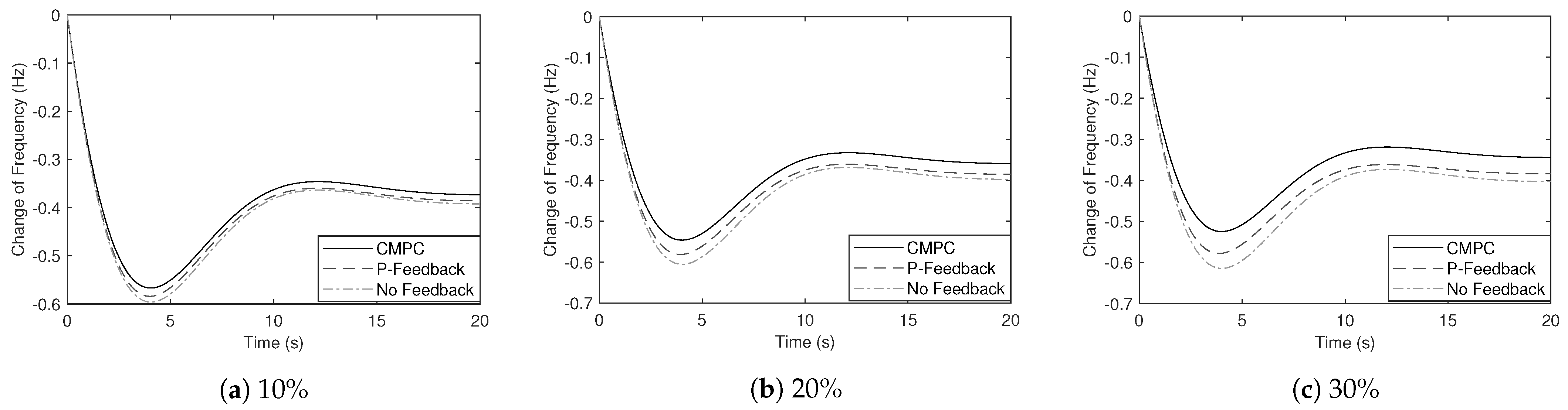
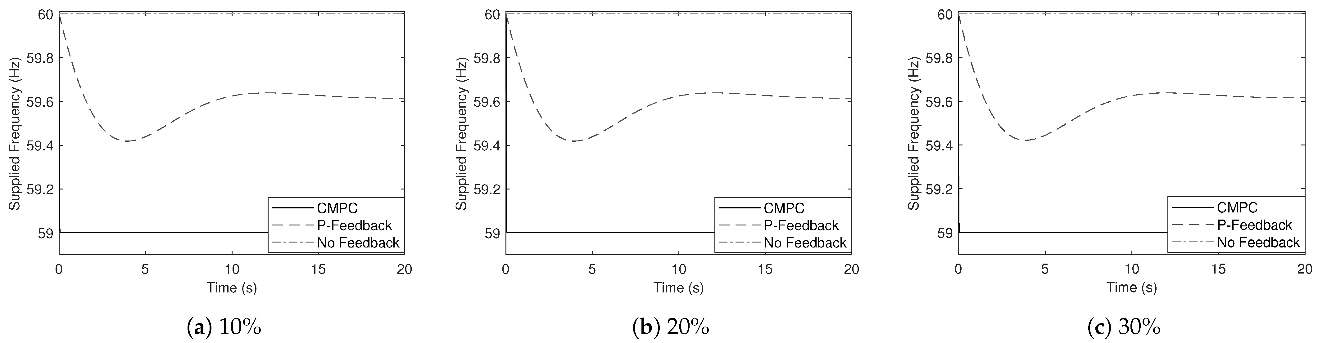
Three scenarios of SSTs’ integration and three scenarios of SST’s control are investigated to exhibit the performance of the proposal. These consider 10%, 20% and 30% of integration. In terms of the SST control, the natural response of the system with no SST integration (No feedback), the SST proportional control strategy (P-Feedback) and the proposed SST control method (CMPC) will be displayed comparatively. Note that, regardless of the SST penetration scenario, the “No feedback” response will always consider that the system has no SST integration.
The simulation results are shown in Figure 7, Figure 8, Figure 9 and Figure 10. In Figure 7, the frequency responses are shown.
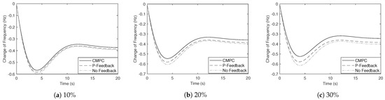
Figure 7.
System frequency response under a power loss of 2 GW.
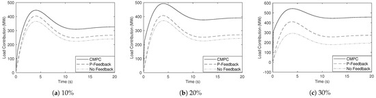
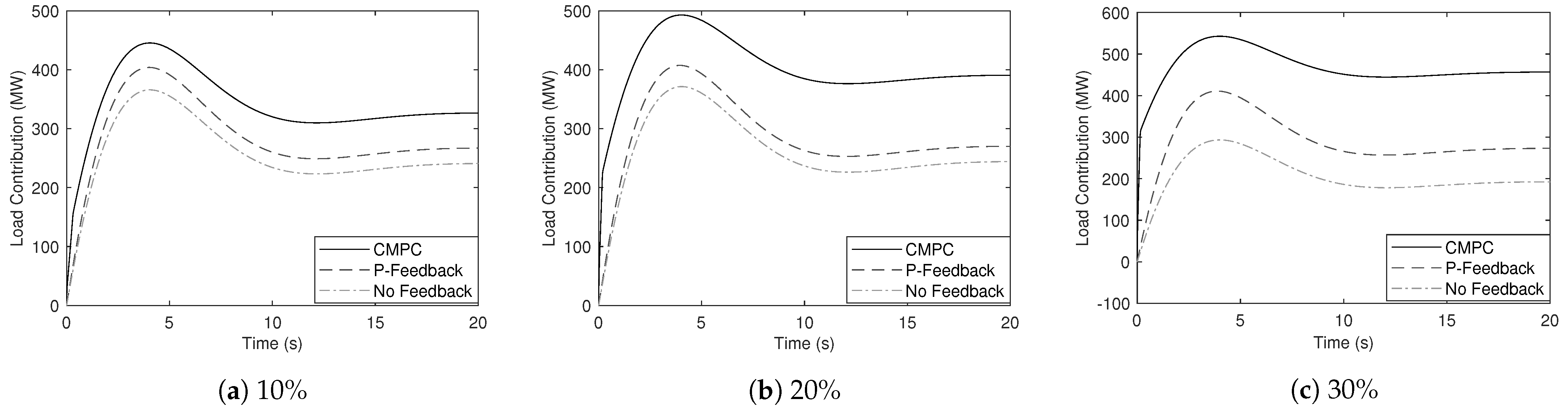
Figure 8.
Load response under a 2GW power loss.
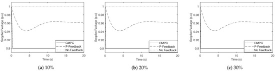
Figure 9.
Supplied voltage under a 2GW power loss.
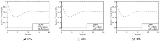
Figure 10.
SST supplied frequency under a 2GW power loss.
The CMPC response in Figure 7 is, overall, better than both the natural response and the proportional control. In terms of ROCOF, the improvement is not significant, meanwhile the improvement of the NADIR point is noticeable with about 1 dHz for a 30% of SST penetration. This result is consistent with the objective of the control action in minimizing the NADIR value.
The load response is exhibited in Figure 8. The better NADIR response comes from a larger contribution of loads to reestablish the power balance. It is important to note that the SST control leads to a load response that is superior to the proportional control, which emphasizes the optimality of the proposed approach that translates into a larger and faster power response from loads.
The output voltage of the SST is shown in Figure 9. For the “no feedback” case, the voltage magnitude is left constant as no SST integration is considered in this particular scenario. In the case of proportional control feedback, the voltage is proportional to the frequency in the system. Meanwhile, in the incorporation of the CMPC-based controller, the control action drives the voltage directly to the lower possible value within the grid code limits, allowing a much faster and effective response.
The frequency output of the SST is depicted in Figure 10. For the “no feedback” case, the magnitude is left constant as no SST integration is considered in this particular scenario. For the case of proportional feedback, the frequency is just the frequency of the system. For the case of CMPC, the control action drives the frequency directly to the lower possible value within the grid code limits, allowing a much faster and effective response, analogous to the voltage response. Note that Figure 10 shows the frequency that is supplied by the SST to the feeder, different from the frequency that occurs in the transmission level within the power system. This is consistent with the fact that the SST decouples the load-frequency dynamics of distribution loads from that of the power system.
A comparative analysis of the ROCOF and NADIR values is summarized in Table 4. The emphasis of the control on NADIR is evident as the most significant differences can be associated with NADIR results.
Table 4.
NADIR and ROCOF results.
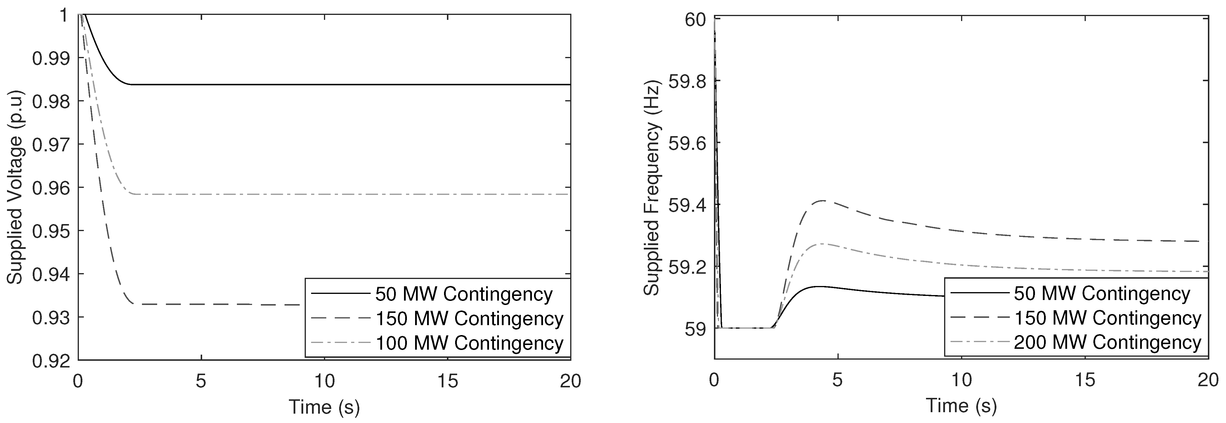
Note that not always the optimal control action will be set to the largest possible movement of SST voltage and frequency. As an example, Figure 11 shows the SST voltage and frequency in the case of the CMPC for power imbalances of lower magnitude than the initial case of 2000 MW, namely 50, 150 and 150 MW.
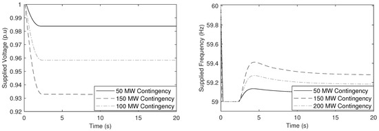
Figure 11.
Supplied voltage and frequency under different levels of contingency.
In Figure 11, the SST voltage is not set to a limit of 0.9 p.u. as in the initial case. This situation is derived from the fact that a smaller contingency requires less power response from loads to be controlled. A similar situation can be observed for the case of the SST frequency. Conceptually, if a larger control action is executed in a fixed manner, the risk of over-frequency events under small power imbalances is evident. The proposed control adapts to the size of the contingency accordingly.
5. Conclusions and Future Works
This paper proposes a predictive control-based frequency response for SSTs. Through simulated scenarios, it was shown that the proposed feedback control achieves higher levels of load contribution due to its optimal formulation, increasing load response from 293 MW in the base case at 30% of SSTs integration to 542 MW with the MPC-algorithm. This led to less serious NADIR excursions, improving about 0.1 Hz for a 30% of SST penetration with respect to the base case with no control. Additionally, the control algorithm explicitly includes constraints of voltage and frequency commonly found in grid codes. Through simulation results, it was demonstrated that those grid code specifications are satisfied. This combination of features cannot be found in the literature of frequency responsive SSTs.
Despite the fact that the proposed control implicitly incorporates the grid code specifications related to the supplied frequency and voltage, future work is proposed to consider ROCOF and voltage derivative constraints aiming to prevent the undesired trigger of anti-island protections and other voltage protections that are common in distribution loads and distributed generators. This representation would require new constraints on the derivative of voltage and frequency.
Another future work consists of considering the distributed nature of SSTs, since the proposed model considers an equivalent representation for SSTs and loads, while there are multiple SSTs in every distribution feeder in actual systems. The proposed control must be tested in a large number of cases to represent this variety of conditions to obtain statistically-significant results.
Similarly, different approaches have taken advantage of the DC-link stored energy to provide some synthetic responses, which may be integrated into the proposed control for enhancing the SST frequency contribution.
Finally, the proposed study considers balanced conditions for loads. Future work is proposed to adapt the formulation to represent unbalanced cases.
Author Contributions
Conceptualization, C.F. and H.C.; methodology, C.F.; software, C.F.; validation, C.F.; formal analysis, C.F.; investigation, C.F.; resources, H.C.; data curation, C.F.; writing—original draft preparation, C.F.; writing—review and editing, M.R.A.P.; visualization, C.F.; supervision, H.C.; project administration, H.C.; funding acquisition, H.C. All authors have read and agreed to the published version of the manuscript.
Funding
This work was supported by ANID-Chile under Fondecyt grant 1191302 and grant ANID-PFCHA/Doctorado Nacional/2020-21200486.
Institutional Review Board Statement
Not applicable.
Informed Consent Statement
Not applicable.
Data Availability Statement
This would be available upon request.
Conflicts of Interest
The authors declare no conflict of interest.
References
- Gonzalez-Longatt, F.M.; Acosta, M.N.; Chamorro, H.R.; Rueda Torres, J.L. Power Converters Dominated Power Systems. In Modelling and Simulation of Power Electronic Converter Dominated Power Systems in PowerFactory; Gonzalez-Longatt, F.M., Rueda Torres, J.L., Eds.; Springer International Publishing: Cham, Switzerland, 2021; pp. 1–35. [Google Scholar]
- Chamorro, H.R.; Torkzadeh, R.; Eliassi, M.; Betancourt-Paulino, P.; Rezkalla, M.; Gonzalez-Longatt, F.; Sood, V.K.; Martinez, W. Analysis of the Gradual Synthetic Inertia Control on Low-Inertia Power Systems. In Proceedings of the 2020 IEEE 29th International Symposium on Industrial Electronics (ISIE), Delft, The Netherlands, 17–19 June 2020; pp. 816–820. [Google Scholar] [CrossRef]
- Denholm, P.; Mai, T.; Kenyon, R.W.; Kroposki, B.; Malley, M.O. Inertia and the Power Grid: A Guide without the Spin; Technical Report NREL/TP-6120-73856; National Renewable Energy Laboratory: Golden, CO, USA, 2020.
- Thiesen, H.; Jauch, C. Determining the Load Inertia Contribution from Different Power Consumer Groups. Energies 2020, 13, 1588. [Google Scholar] [CrossRef] [Green Version]
- Obaid, Z.A.; Cipcigan, L.M.; Abrahim, L.; Muhssin, M.T. Frequency control of future power systems: Reviewing and evaluating challenges and new control methods. J. Mod. Power Syst. Clean Energy 2019, 7, 9–25. [Google Scholar] [CrossRef]
- Rojas, F.; Diaz, M.; Espinoza, M.; Cárdenas, R. A solid state transformer based on a three-phase to single-phase modular multilevel converter for power distribution networks. In Proceedings of the 2017 IEEE Southern Power Electronics Conference (SPEC), Puerto Varas, Chile, 4–7 December 2017; pp. 1–6. [Google Scholar]
- Kolar, J.W.; Ortiz, G. Solid-state-transformers: Key components of future traction and smart grid systems. In Proceedings of the International Power Electronics Conference-ECCE Asia (IPEC 2014), Hiroshima, Japan, 18–21 May 2014; pp. 18–21. [Google Scholar]
- Baier, C.R.; Torres, M.A.; Perez, M.A.; Cárdenas, R.; Ramirez, R.; Melín, P. Hybrid Transformers with Virtual Inertia for Future Distribution Networks. In Proceedings of the 45th Annual Conference of the IEEE Industrial Electronics Society (IECON 2019), Lisbon, Portugal, 14–17 October 2019; Volume 1, pp. 6767–6772. [Google Scholar] [CrossRef]
- Khodabakhsh, J.; Moschopoulos, G. Primary Frequency Control in Islanded Microgrids Using Solid-State Transformers as Virtual Synchronous Machines. In Proceedings of the 2020 IEEE Energy Conversion Congress and Exposition (ECCE), Detroit, MI, USA, 11–15 October 2020; pp. 5380–5385. [Google Scholar] [CrossRef]
- De Carne, G.; Buticchi, G.; Liserre, M.; Vournas, C. Real-Time Primary Frequency Regulation Using Load Power Control by Smart Transformers. IEEE Trans. Smart Grid 2019, 10, 5630–5639. [Google Scholar] [CrossRef] [Green Version]
- Langwasser, M.; De Carne, G.; Liserre, M. Smart Transformer-based Frequency Support in Variable Inertia Conditions. In Proceedings of the 2019 IEEE 13th International Conference on Compatibility, Power Electronics and Power Engineering (CPE-POWERENG), Sonderborg, Denmark, 23–25 April 2019; pp. 1–6. [Google Scholar] [CrossRef]
- Rodrigues, J.; Moreira, C.; Lopes, J.P. Smart Transformers as Active Interfaces Enabling the Provision of Power-Frequency Regulation Services from Distributed Resources in Hybrid AC/DC Grids. Appl. Sci. 2020, 10, 1434. [Google Scholar] [CrossRef] [Green Version]
- Li, Y. Stability and Performance of Control Systems with Actuator Saturation, 1st ed.; Control Engineering; Springer International Publishing: Cham, Switzerland, 2018. [Google Scholar]
- Fang, J.; Li, H.; Tang, Y.; Blaabjerg, F. On the inertia of future more-electronics power systems. IEEE J. Emerg. Sel. Top. Power Electron. 2018, 7, 2130–2146. [Google Scholar] [CrossRef]
- Chavez, H.; Baldick, R.; Sharma, S. Regulation Adequacy Analysis Under High Wind Penetration Scenarios in ERCOT Nodal. IEEE Trans. Sustain. Energy 2012, 3, 743–750. [Google Scholar] [CrossRef]
- National Grid. Operational Strategy Report 2021. Available online: https://www.nationalgrideso.com/research-publications/system-operability-framework-sof (accessed on 1 November 2021).
- Arif, A.; Wang, Z.; Wang, J.; Mather, B.; Bashualdo, H.; Zhao, D. Load Modeling—A Review. IEEE Trans. Smart Grid 2018, 9, 5986–5999. [Google Scholar] [CrossRef]
- Choi, B.K.; Chiang, H.D.; Li, Y.; Chen, Y.T.; Huang, D.H.; Lauby, M.G. Development of composite load models of power systems using on-line measurement data. In Proceedings of the 2006 IEEE Power Engineering Society General Meeting, Montreal, QC, Canada, 18–22 June 2006. [Google Scholar]
- Shamshuddin, M.A.; Rojas, F.; Cardenas, R.; Pereda, J.; Diaz, M.; Kennel, R. Solid State Transformers: Concepts, Classification, and Control. Energies 2020, 13, 2319. [Google Scholar] [CrossRef]
- Kazmierkowski, M.P. Power Converters and AC Electrical Drives with Linear Neural Networks (Cirrincione, M., et al; 2012) [Book News]. IEEE Ind. Electron. Mag. 2013, 7, 61. [Google Scholar] [CrossRef]
- Wang, L. Continuous time model predictive control design using orthonormal functions. Int. J. Control 2001, 74, 1588–1600. [Google Scholar] [CrossRef]
- Wang, L. Model Predictive Control System Design and Implementation Using MATLAB®; Springer Science & Business Media: London, UK, 2009. [Google Scholar]
- Western Power Distribution. Project Network Equilibrium Voltage Limits Assessment Discussion Paper. Available online: https://www.westernpower.co.uk/downloads-view-reciteme/2503 (accessed on 1 November 2021).
- Fuentes, C.; Riquelme, E.; Chavez, H. Towards Distribution Feeders Frequency Response via Solid State Transformers. In Proceedings of the 2020 IEEE PES Transmission Distribution Conference and Exhibition Latin America (T D LA), Montevideo, Uruguay, 28 September–2 October 2020; pp. 1–6. [Google Scholar] [CrossRef]


Publisher’s Note: MDPI stays neutral with regard to jurisdictional claims in published maps and institutional affiliations. |
© 2021 by the authors. Licensee MDPI, Basel, Switzerland. This article is an open access article distributed under the terms and conditions of the Creative Commons Attribution (CC BY) license (https://creativecommons.org/licenses/by/4.0/).