1. Introduction
Despite an unprecedented 5.8% decrease in global CO
2 emissions in 2020 due to the COVID-19 pandemic causing a reduction in energy demand, Total Greenhouse Gas Emissions (TGGEs) are expected to rebound by nearly 5% in 2021, approaching the 2018–2019 peak. This increase is mainly attributable to the economic rebound of developing and emerging economies, responsible for over two-thirds of global CO
2 emissions. Conversely, TGGEs are in a structural decline in advanced economies [
1]. In the last decades, the governments of developed countries have indeed supported the implementation of national climate policies to achieve a drastic reduction in TGGEs from anthropogenic activities by 2050. Renewable energy sources (RESs) constitute the mainstay of developed country energy policies for achieving this goal. Among RESs, biomass energy sources have received significant attention due to their characteristics of environmental and economic sustainability, as well as their abundance in nature [
2].
In this context, biomass gasification as a conversion technology is becoming increasingly important on account of its renewability and environmental benefits, as well as its sociopolitical benefits [
3]. Biomass gasification is expected to play a crucial role in supplying the energy demand in many countries, being one of the economically attractive technologies for the production of clean energy. The major advantage of the gasification process is that it allows for the conversion of waste biomass and other similar biodegradable wastes, which would otherwise have been discarded and unused, into valuable fuel. The synthesized gas produced through biomass gasification is suitable for multiple applications as it can be (i) burned at higher temperatures, (ii) employed in fuel cells, (iii) employed to produce methanol and hydrogen and (iv) converted via the Fischer–Tropsch process into a range of synthesized liquid fuels suitable for use in gasoline or diesel engines [
4]. The by-products (e.g., biochar, tar) derived from the gasification process can also be used in multiple ways. For example, biochar can be employed as fertilizer in agriculture, filter absorber in industrial or energy carriers [
5], and recently, some researchers have investigated the feasibility of using biochar as a carbon sequestering additive in cement mortar [
6]. Furthermore, the gasification process allows the use of a variety of biomass resources as feedstocks, including wood material, pulp and paper industry residues, agricultural residues, organic municipal material, sewage, manure, and food processing by-products. A great number of agricultural cultivation residues such as straws, nutshells, fruit shells, fruit seeds, plant stalks and stover, green leaves, and molasses are globally produced each year [
7]. For example, 89.5 million tones of rapeseed were cultivated worldwide in 2017 [
8]. Rapeseed plantations entail the production of a large quantity of straw that needs to be disposed of, and since disposal via open field burning causes air pollution, the use of a gasification technology can have a reduced environmental impact and fewer consequences for the environment than landfill operations or combustion of the waste. For these reasons, in the last decades, gasification became reputed as a valuable solution for disposal of refuse-derived fuel from municipal solid waste, especially in developing countries [
9].
The thermochemical conversion process of gasification is a mature, reliable and flexible technology, well known and described extensively in the literature [
10,
11,
12,
13]. Even though biomass gasification is a mature technology, some technological barriers limit its large-scale commercial development. It has been observed that the main constraints in the implementation of biomass gasification are represented by: (i) the variability of biomass feedstock physical properties, which requires high flexibility of the gasifier, (ii) the high moisture content of biomass, which decreases the energy efficiency of the process, (iii) the production of ash during the process, which can cause air pollution, (iv) the presence of tar in the end products, which has a tendency to cause fouling and plugging in the plant pipes and (v) the handling and management of biomass feedstock [
14]. In order to overcome some of the aforementioned technological barriers, a deep understanding of the different phenomena and operational parameters involved in gasification process is required. To this aim, mathematical modeling is a useful tool to understand physical and chemical mechanisms that occur inside the gasifier. A numerical model allows for the evaluation of process performance when varying the biomass proprieties and operating parameters, providing a set of optimum operating conditions and designating the risks and limits of the system. Additionally, a numerical model helps to considerably reduce the costs of research and development of new and innovative devices [
15].
Mathematical models for biomass gasification process can be categorized into: (i) thermodynamic equilibrium models, (ii) kinetic rate models, (iii) computational fluid dynamics models (CFD), and (iv) artificial neural networks (ANNs) models. Thermodynamic equilibrium models are based on the assumption that the system of chemical reactions involved in the process reaches a state of thermochemical equilibrium inside the gasifier reactor [
16]. Equilibrium models are able to predict the producer gas composition, the maximum yield and the optimal conditions of energy efficiency and syngas heating value for the operation of each specific reactor according to biomass feedstock properties [
10,
11]. This approach does not require details of system geometry or estimation of the necessary time to reach equilibrium [
17]. Kinetic models are based on mathematical description of the reaction kinetics of the main reactions and the hydrodynamic phenomena among phases that occur inside the gasification reactor [
13]. Such models are able to predict the trend and composition of the product in different positions within the reactor, as well as the overall gasifier performance as a function of the operating conditions and configuration of the gasifier [
18]. Application of kinetic models involves knowledge of the reaction rate, residence time, reactor hydrodynamics (e.g., superficial velocity, diffusion rate) and gasifier geometry. The key issues with kinetic modeling are the associated high cost for computation and the use of parameters that make it difficult to apply to different plants [
19]. Computational fluid dynamics (CFD) modeling is one of the most advanced tools for the analysis of the gasification process. CFD simulations provide the temperature profiles of the gasifier, solid and gas phases, as well as a complete chemical and fluid mechanical analysis of the reactor bed. CFD analysis can be used for optimization of the gasifier design and to study characteristics of the gasification process such as operating parameters, kinetics and physical properties of the feedstock. However, comprehensive CFD simulations for biomass gasification are scarce, mainly due to the lack of large computational resources and the anisotropic nature of biomass [
10]. Artificial neural network (ANN) models are a relatively new approach to model the gasification process. ANN models are able to predict gas yield and syngas composition with sufficient accuracy [
20]. Such models do not provide an analytical solution, only numerical results [
11], and do not require mathematical description of the phenomena occurring in the process. For this reason, they constitute a useful tool for simulating and scaling the complex biomass gasification process. Nevertheless, the application of ANN for biomass gasification is rather rare [
20].
The choice of the most suitable modeling approach to investigate the biomass gasification process is determined by the scope of the analysis and the available experimental data. Complex models (e.g., kinetic, CDF, and ANN models) provide detailed information on mechanisms. However, the computational cost and the number of input data required are usually very high. Although equilibrium models are valid only under chemical equilibrium conditions, they are valuable because they can predict the thermodynamic limits of a gasification system, leading to the design, evaluation and improvement of the process. Furthermore, equilibrium models can constitute useful design support in evaluating the possible limiting behavior of a complex system that is difficult or unsafe to reproduce experimentally or in commercial operation [
18]. In fact, thanks to the relative simplicity of equilibrium models and the very low computation requirements, they could represent a very useful design and optimization tool for conversion systems fed by biomass.
The purpose of this paper is to present an overview of thermodynamic equilibrium models. In particular, the aim is to assess the reliability of equilibrium models for the simulation of the gasification process as a function of biomass properties and operating conditions. The work presented in this paper represents a preliminary step in the development of a useful tool for the design and optimization of polygeneration systems and their interaction with smart energy grids. In fact, this study is aimed at establishing a basis for the development of efficient modeling tools that will be employed to build new control and optimization schemes and operating maps of biomass gasification systems integrated in polygeneration plants, coupled with energy networks. The main objective of the present paper consists of the assessment of thermodynamic equilibrium models as a function of biomass type and composition in order to better understand in which conditions of practical interest such models can be applied with acceptable reliability, even neglecting tar and char formation to minimize model complexity. Indeed, in case of the analysis of complex energy systems as polygeneration plants, a simple and flexible model can represent an easily usable tool for the evaluation of optimal process parameters. To this aim, the authors developed two equilibrium models using both commercial software and (referred as Aspen model) a simulation tool implemented in a non-commercial script (referred as mathematical model). The developed models were applied to a large number of experimental case studies available in the scientific literature, assessing thermodynamic equilibrium models’ performance for gasification of different biomasses and in different operating conditions. Such analysis is crucial for the development of a numerical tool for the simulation of complex energy conversion systems with the capability to produce results in a very short time and that can be employed not only in the design stage, but also in the plant optimization and monitoring stages. To the authors’ knowledge, very few papers are available in the scientific literature giving such an analysis.
2. Overview of Biomass Gasification Equilibrium Models
The thermodynamic equilibrium approach is based upon the assumption that the components react in a fully mixed steady state condition This assumption can be considered realistic when the residence time of the reactants in the gasification zone is long compared to the half-life of all the reactants, gasification temperature can be assumed as constant, and chemical mixing is almost perfect [
21]. These conditions are met in some specific types of reactors, mainly in downdraft fixed-bed reactors, and at high temperatures (e.g., >1500 K) [
22]. However, the equilibrium state may not be reached in some gasifiers and under specific operative conditions, in particular for gasifiers in which the operating temperatures are relatively low. Nonetheless, thermodynamic equilibrium models have been extensively employed to investigate the biomass gasification process [
23].
Equilibrium models can be further categorized as non-stoichiometric or stoichiometric equilibrium approaches. Stoichiometric models are adapted from the equilibrium constants of a set of reactions [
19], while nonstoichiometric models are based on the Gibbs free energy minimization approach. This formulation requires only the elemental composition of the biomass as input; therefore, it is particularly suitable for cases in which the system of chemical reactions that take place in the gasifier is not fully known [
11]; while for the application of the stoichiometric equilibrium models, the knowledge of the main chemical reactions and species involved in the process is required.
Zainal et al. [
24] proposed a stoichiometric equilibrium model for a downdraft gasifier, investigating the effects of initial moisture content in the biomass feedstock and the temperature in the gasification zone on the producer gas composition and the calorific value.
Li et al. [
25] developed a thermodynamic equilibrium model based upon the minimization of Gibbs free energy to predict the performance of a circulating fluidized bed gasifier. The authors proposed a phenomenological model modifying a previous model through the introduction of an availability function that used empirical data (e.g., unconverted carbon and methane) to consider the non-equilibrium factors.
Sharma [
26] presented a stoichiometric equilibrium model of the global reduction reactions for char–gas and gas–gas reactions that occur in the reduction zone of a downdraft gasifier. In order to accurately predict the reaction temperature, the model considered the heat exchanges that take place in the reduction zone using energy equations. The results showed reasonable agreement with data collected from various sources for downdraft biomass gasifiers.
Jarungthammachote et al. [
27] employed a thermodynamic equilibrium model based upon the equilibrium constants to predict producer gas composition. In order to improve the accuracy of simulation results, the authors modified the model by multiplying the equilibrium constant with appropriate coefficients calculated on the basis of experimental data.
Baratieri et al. [
28] presented an equilibrium model for the biomass gasification process modified based on experimental data. The model was calibrated using concentrations of CH
4 and C
2H
4 measured experimentally and the amount of char residue. The results of the modified model accurately predicted the syngas composition for the gasification process in the analyzed fluidized gasifier.
Barba et al. [
29] developed the Gibbs Free Energy Gradient Method Model (GMM). The gasification process was modeled in two steps: in the first step, the raw material was decomposed to produce a carbonaceous residue and a primary gas. In the second stage, the gas previously produced changed its composition due to the occurrence of water shift and steam reforming reactions.
In [
30], the GMM thermodynamic model was employed to simulate an experimental campaign carried out at the ENEA Research Centre of Trisaia (Rotondella, Italy), which showed good accuracy in reproducing the experimental results of steam gasification of refuse-derived fuel.
An advanced two-stage fluidized bed gasification was modeled by Materazzi et al. [
31] using a non-stoichiometric approach. The model had a systematic structure consisting of principles of atomic conservation and equilibrium calculation routines. The model was validated through employing experimental data from a pilot plant.
Sreejith et al. [
32] presented an equilibrium model for the steam gasification of biomass based upon the minimization of Gibbs free energy to identify the optimum values for the reactor when varying temperature and pressure. The gas phases were modeled as real gases in accordance with the Redlich–Kwong equation of state. Kangas et al. [
33] developed a non-stochiometric equilibrium model with the constrained Gibbs energy method. The assumed chemical system consisted of 14 constituents in the gaseous phase, the liquid water phase, and two solid phases for char and ash. Six methods for modeling global or local equilibrium were implemented by varying the constrained species.
Mendiburu et al. [
34] developed four thermodynamic equilibrium models for the downdraft gasifiers, called M1, M2, M3, and M4. The first model, M1, was a general stoichiometric equilibrium model. Models M2, M3, and M4 were obtained by modifying model M1. In particular, in model M2 two multiplicative coefficients calculated using experimental data were introduced into the equilibrium equations. Model M3 implemented the correlations for CO/CO
2 and CO/H
2 according to [
35]. Model M4 implemented the substitution of the formula for the calculation of equilibrium constants with the Arrhenius type relations.
To improve accuracy in the prediction of pyrolysis products, Biagini et al. [
36] developed a multizonal model adapted from the non-stoichiometric equilibrium approach. The proposed model simulated the bypass of the oxidation zone by some products of the pyrolysis phase inside the gasifier through introducing a repartition coefficient of the volatile matter.
Gagliano et al. [
37] presented a stoichiometric model to simulate the gasification process through a downdraft gasifier filled with residual biomasses. The proposed model could predict the percentage of tar and char produced, as well as the chemical species in the producer gas. A good agreement between experimental data and simulation data was found.
Gambarotta et al. [
38] developed a thermodynamic equilibrium model for the biomass gasification process in downdraft gasifiers. The model was able to predict not only the concentration of the main component of syngas but also the content of minor products, especially pollutant substances containing nitrogen and sulfur (e.g., ammonia, hydrogen sulfide).
Regarding the simulation of the entire gasification process, it is often advantageous to use process simulators (e.g., Aspen Plus, HYSYS, ChemCad, etc.). Among commercial software, Aspen Plus is one of the most common process simulation tools used to simulate biomass gasification and assess the performance of the overall process of gasification [
22,
39].
Although Aspen Plus simulation software is quite costly, it was chosen for the simulation process due to its high flexibility concerning the different process configurations, which allows the optimization of the different operating conditions and determination of the limits of the processes under these conditions. In addition, it allows for the avoidance of complex processes and the development of the simplest possible model; it is therefore used to facilitate the calculation of physical and chemical factors in the process. Several Aspen Plus simulation models presented in the literature study the effect of different operating variables on the performance of the process.
Mansaray et al. [
40] developed two models for gasification of rice husks in a fluidized-bed gasifier using Aspen Plus: a one-compartment model, in which the hydrodynamic complexity of the fluidized-bed gasifier was neglected and a global equilibrium approach was used, and a two-compartment model, in which the complex hydrodynamic conditions were considered.
Mathieu and Dubuisson [
41] developed a gasification model using Aspen Plus based on Gibbs free energy minimization and divided into pyrolysis, combustion, Boudouard reaction, and gasification.
Mitta et al. [
42] presented a model of fluidized-bed gasification using Aspen Plus divided into three different phases: drying, devolatilization–pyrolysis, and gasification. A global equilibrium approach was used in the model, omitting the hydrodynamic characteristics.
Nikoo and Mahinpey [
43] modeled a fluidized-bed gasifier by considering kinetic characteristics, employing four models from Aspen Plus with the reactor and external subroutines written in FORTRAN to simulate the gasification process.
Ramzan et al. [
44] proposed a gasification model of different biomasses: food waste, municipal solid waste, and poultry waste. The model was validated with data obtained experimentally.
Kuo et al. [
45] modeled raw bamboo gasification in a downdraft gasifier in Aspen Plus, while Tavares et al. [
46] modeled the gasification process in Aspen Plus using forest residues as fuel and carried out a sensitivity analysis.
Atnaw et al. [
47] modeled the gasification of oil-palm fronds. The authors highlighted that the mass fractions of carbon monoxide, hydrogen and methane were higher at a lower air–fuel ratio, higher oxidation temperature, and lower operating pressure. A similar relationship between the mass fraction of the fuel components and the conditions of pressure and air–fuel ratio was observed by Paviet et al. [
48], where the gasification of wood was investigated. Gagliano et al. [
49] found that the production of CO and H
2 increased not only with a decrease in the air–fuel ratio but also when the process temperature increased. Other strategies to improve gasification performance were found by [
41], such as the preheating of the air used as a gasifying agent up to 300°C and its enrichment with oxygen. The effect of air preheating was demonstrated to be more significant at a low equivalence ratio [
50].
Aspen Plus has been used not only to optimize biomass gasification but also to investigate systems that integrate this process with energy production technologies, such as internal combustion engines, gas turbines, and fuel cells. Násner et al. [
51] used syngas produced via gasification of refuse-derived fuel in a pilot plant in an internal combustion engine, finding that despite the somewhat lower heating value, clean gas could be successfully used for power generation, maintaining reasonable efficiency. The majority of the works where Aspen Plus is used to investigate biomass gasification present a similar approach: the simulation is steady-state, biomass is decomposed into its elements by specifying yield distribution, gasification is based on the minimization of Gibbs free energy, and tar formation is neglected. Some authors developed new approaches starting from the conventional one. Adnan et al. [
52] considered tar formation as furan (C
4H
4O) and calculated its amount through solution of the elemental balances. Other authors, such as Acar and Böke [
53], proposed a restricted chemical equilibrium method where experimental data are used to calibrate the model results by defining a temperature for certain gasification reactions. They applied the temperature approach to carbon reactions which involve carbon and oxygen and carbon and water, the shift reaction, and the steam-reforming reaction related to methane and water. Han et al. [
54] applied the restricted chemical equilibrium to all of the reduction reactions, whereas Gagliano et al. [
49] considered it only for the water–gas shift and methanation reactions.
3. Materials and Methods
As explained in previous sections, the authors developed two thermodynamic equilibrium models using both commercial software, i.e., Aspen Plus®, and a simulation tool implemented in a non-commercial script. In the following, the commercial software-based model is referred to as “Aspen model”, whereas the non-commercial tool is referred to as “Analytical model”.
3.1. Analytical Model
In the present paper the authors propose an analytical model able to predict gasification through the average temperature of the biomass bed and the composition and flow rate of the synthesis gas produced as well as its energy content. The proposed model describes the process of biomass gasification using a concentrated parameter approach [
55,
56].
The hypotheses at the core of the model are: (i) steady state; (ii) uniform and constant properties of biomass inside the gasifier; (iii) local thermodynamic equilibrium; (iv) complete chemical reactions (i.e., the reactions taking place completely stoichiometrically); (v) uniform and constant temperature of biomass bed. Input data for calculation are: (i) mass flow rate of biomass feedstock; (ii) temperature and volumetric flow rate of combustion air; (iii) biomass composition.
For modeling purposes, the chemical formula of the biomass is defined as
, where
x,
y and
z are the number of hydrogen, oxygen and nitrogen atoms per number of carbon atoms in the feedstocks, respectively [
57]. The latter is calculable knowing the elemental composition of biomass based on the ultimate and proximate analyses.
Assuming thermodynamic equilibrium, the biomass gasification process is modeled according to the following global reaction:
where
w is the amount of moisture per mole of carbon and
m = O/C is the amount of oxygen per mole of carbon. The number of moles of the different species,
ni, on the right hand side represents the unknown quantities of the problem. The produced moles of H
2, CO, CO
2, H
2O and CH
4 are determined by solving five simultaneous equations. The first three equations are related to the mass balance of the involved chemical elements as shown in Equations (2)–(4) [
57,
58,
59].
The two additional equations were obtained under the assumption of chemical equilibrium and minimizing Gibbs free energy relative to the methanation reaction:
and to the water–gas shift reaction:
The equilibrium constants for reactions (5) and (6) are given by the following equation [
56,
57,
60]:
where
is the universal gas constant,
is the standard Gibbs function of reaction,
is the temperature and
is the standard Gibbs function of formation of the gaseous species in the producer gas at temperature the
T. The latter can be evaluated employing the empirical equation below:
The values of coefficients
and
are reported in [
57] for the
i-th component involved (i.e., CO, CO
2, CH
4, H
2O).
In this model, thermodynamic equilibrium is assumed for all chemical reactions in the gasification zone. Moreover, all gases are assumed to be ideal and all reactions to form at a pressure of 1 atm. Therefore, the equilibrium constants for the methanation reaction and water–gas shift reaction are given by the ensuing equations [
27,
61,
62]:
Water–gas shift reaction:
where
xi is the mole fraction of species i in the ideal gas mixture,
ν is the stoichiometric number (positive value for products and negative value for reactants),
p0 is the standard pressure and
ntotal is the total mole of producer gas. Using Equations (9) and (10), it is possible to calculate the concentration of products and reactants. Mass balances and chemical equilibrium relations equations are solved together with the energy conservation equation for the gasification process, allowing for prediction of the gasification temperature. The energy balance for this process can be written as:
where
and
are the formation enthalpy of organic matter and water at reference condition (298 K and 101325 Pa) in kJ/kmol, respectively;
represents the number of moles produced for the same chemical species per mole of consumed fuel; lastly,
is the enthalpy associated with the
i-th chemical species at temperature
T and it is the sum of the formation enthalpy and the difference in enthalpy between the state in which the substance is found and the reference status.
The enthalpy of formation for organic matter,
, in the reactant is calculated according to the equation suggested in [
27]:
where
is the lower heating value of the dry fraction of biomass estimated in accordance with the formula reported in [
27]:
where
is the mass fraction of hydrogen in the biomass,
is the enthalpy of vaporization of water at reference conditions and
is the higher heating value calculated on the basis of biomass composition conforming to the following equation [
61]:
where
and
are the mass fractions of carbon, hydrogen, oxygen, nitrogen, sulfur and ash in the biomass.
The calculation of the temperature, chemical composition and volumetric flow rate of the syngas produced from the biomass gasification process is based on an iterative process. Namely, the calculation procedure is based on the following steps: (i) an average gasification temperature of the first attempt is assumed; (ii) the mass conservation and chemical equilibrium equations are solved using the Newton–Rapson method [
61] by means of obtaining the composition of the producer gas; (iii) the energy conservation equation is solved, determining the new average gasification temperature; (iv) the iterative method ends when convergence is achieved.
3.2. Aspen Model
A numerical model to simulate downdraft gasification was developed through the commercial software Aspen Plus. Although Aspen Plus provides many built-in unit operation blocks, a component to simulate the gasification process was not available. For this reason, as commonly proposed in the literature [
39], gasification modeling was carried out by combining a component based on the minimization of the Gibbs free energy together with other blocks provided by Aspen Plus and some external subroutines written in FORTRAN. A scheme of the model developed in Aspen Plus is reported in
Figure 1.
This simulation model in Aspen Plus was initially developed for the calculation of coal gasification but was extended to biomass using the same approach. For both coal and biomass, proximate and ultimate analyses were used for the input data.
The fuel (BIOMASS) is fed into a decomposition reactor, an RYield reactor (DECOMP) used to decompose non-conventional streams, such as biomass, into their constituent elements (C, H2, N2 and O2), water, and ash. The reactor that simulates chemical equilibrium by minimizing Gibbs free energy cannot deal with non-conventional components. The RYield reactor is used as a decomposition block since stoichiometry and kinetics are unknown, but a yield distribution is available. The mass yields of the RYield reactor are determined and set based on data from ultimate and proximate analyses using a subroutine written in FORTRAN.
The outlet stream from the decomposition block (DEC-FEED) enters a separator, a block SSplit (S-CHAR), to remove unreacted char before the gasification reactor (C-CHAR). For the gasification reactor, an RGibbs (GASIFIER) is used, into which the decomposed biomass without unreacted char (GASFEED) and the gasifying agent (AIR) are fed.
The unconverted char is heated to the gasifier temperature (H-CHAR), using a Heater block (C-HEATER), and then mixed with the gas stream, leaving the gasifier (RAW-SYNGAS) in a Mixer block (MIXER). Finally, the unreacted char and ash (ASH-CHAR) are separated from the SYNGAS through a FILTER using a Sep block. A brief description of the operations blocks is reported in
Table 1.
Biomass is modeled as a carbonaceous fuel [
63] and its density and enthalpy are calculated through statistical correlations based on the biomass’s ultimate, proximate, and sulfur analyses [
64]. In Aspen Plus such materials are modeled as “non-conventional” streams. Since the process also includes conventional materials (e.g., gas, liquid, and solid), the MIXCINC stream class is considered in this work. The calculation of all the thermodynamic properties is carried out through the Peng Robinson–Boston Mathias modified method, which is suitable for modeling multiple phases, as well as conventional and nonconventional solids and high-temperature processes.
The following assumptions are considered for the simulation of biomass gasification: (i) the process is considered to be steady-state; (ii) gasification is assumed to be run isothermally; (iii) the model is zero-dimensional and kinetic-free; (iv) biomass devolatilization occurs instantaneously at the entrance of the reactor; (v) the char contains only carbon; (vi) sulfur and nitrogen reactions are not considered; (vii) syngas is modeled as a mixture of hydrogen (H
2), carbon monoxide (CO), carbon dioxide (CO
2), methane (CH
4) and moisture (H
2O); (viii) pressure for all components is set to atmospheric pressure; (ix) the formation of tars and other heavy products is neglected; (x) heat losses are neglected. Due to the short residence time of gases in the reactor, the gasification process does not straightforwardly reach a chemical equilibrium state. For this reason, Restricted Chemical Equilibrium is implemented, as proposed in [
65], by specifying for each reaction a temperature approach, which represents the difference between the chemical equilibrium temperature and the real reactor temperature. This method is used to simulate the real condition of the gasifier, which is a non-equilibrium condition. This allows for moving the reaction equilibrium towards a reagent or product composition of the syngas closer to the real one. With regard to reactions, in addition to methanation (5) and water–gas shift (6), carbon combustion (15) and hydrogen combustion (16) are considered:
4. Results and Discussion
For the purposes of validating the developed models, evaluating the accuracy of the simulation results when varying the biomass properties and the gasification operating conditions, and evidencing the advantages and disadvantages of employing such models, the developed thermodynamic equilibrium models were applied to different experimental data from downdraft gasifiers available in the scientific literature.
In
Table 2 and
Table 3, the ultimate and proximate analyses of the different types of biomasses used in the experimental campaigns and the operating conditions of the simulated case studies are summarized. Symbols C, H, O, N and S in
Table 1 represent, respectively, the carbon, hydrogen, oxygen, nitrogen and sulfur content in the biomass on a dry basis (d.b.), while VM and FC are the volatile matter and fixed carbon, respectively.
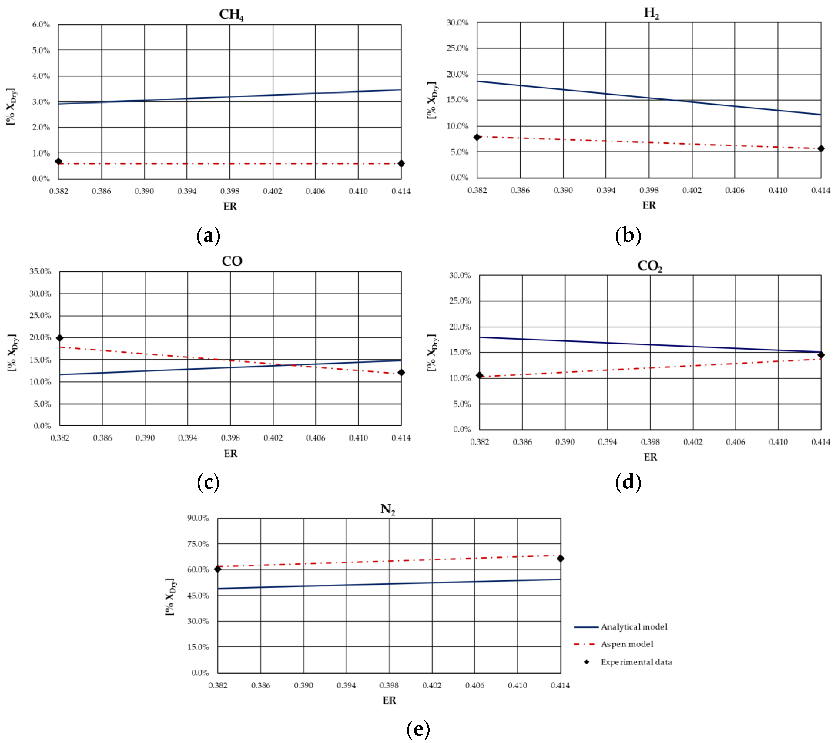
The comparison between numerical and experimental results has been carried out in terms of: (i) molar composition of syngas (e.g., CH
4, H
2, CO, CO
2 and N
2) and (ii) average gasification bed temperature. The comparison was carried out using the data reported in [
66,
69] as these are the only works containing information on the gasification temperature among those considered in this paper.
Present results were obtained by calibrating both the analytical and the Aspen models. Specifically, the analytical model was calibrated by calculating the K1 and K2 values that minimize the error between experiments and model results in terms of gas composition and average combustion bed temperature. Regarding the Aspen model, calibration was based on the Restricted Equilibrium Model (REM).
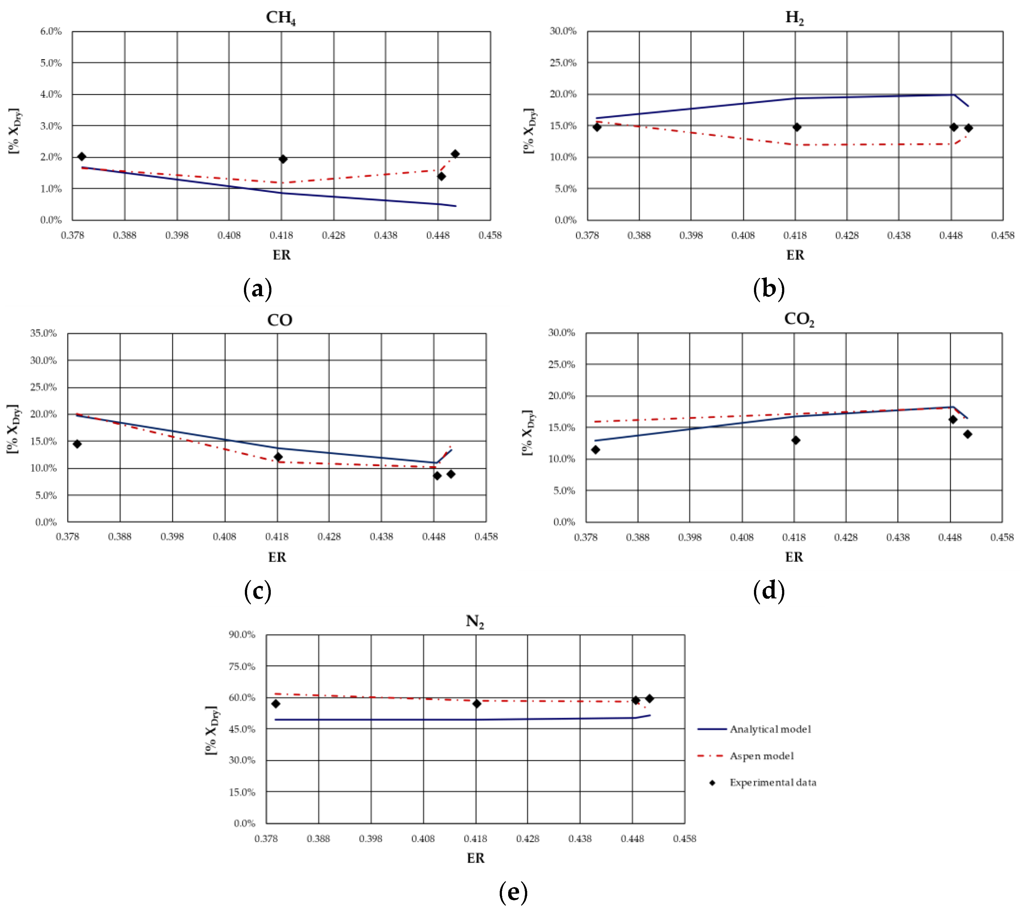
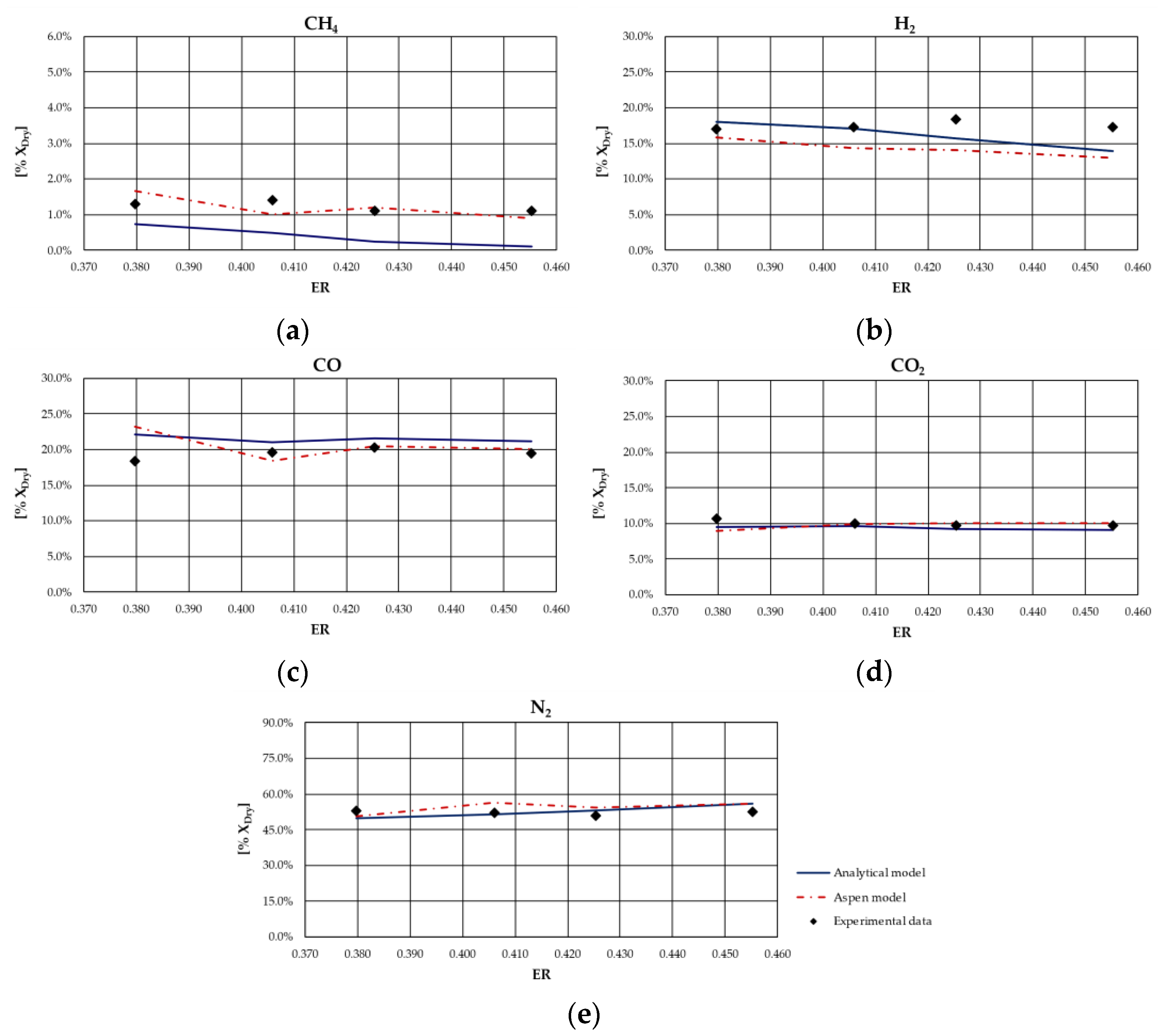
From the analysis of figures and tables, it can be observed that even though the proposed models are both based on the thermodynamic equilibrium hypothesis, significant differences were observed in obtained results. In particular, CH
4 and H
2 molar fractions evaluated using the analytical model were characterized by a higher deviation from experimental values compared to the other synthesized gas components: CH
4 molar concentration was underestimated for case studies in which the ER was higher; conversely, it was overestimated for the case studies in which the ER is lower. Furthermore, CH
4 content decreased as ER increased for all types of biomasses, except for rice husks. The analytical model generally overestimated the H
2 molar fraction regardless of the biomass feedstock and the operating conditions of the gasification process. Good agreement between the results of the analytical model and experimental values could be observed with regard to the CO and CO
2 molar concentrations for all case studies analyzed. The N
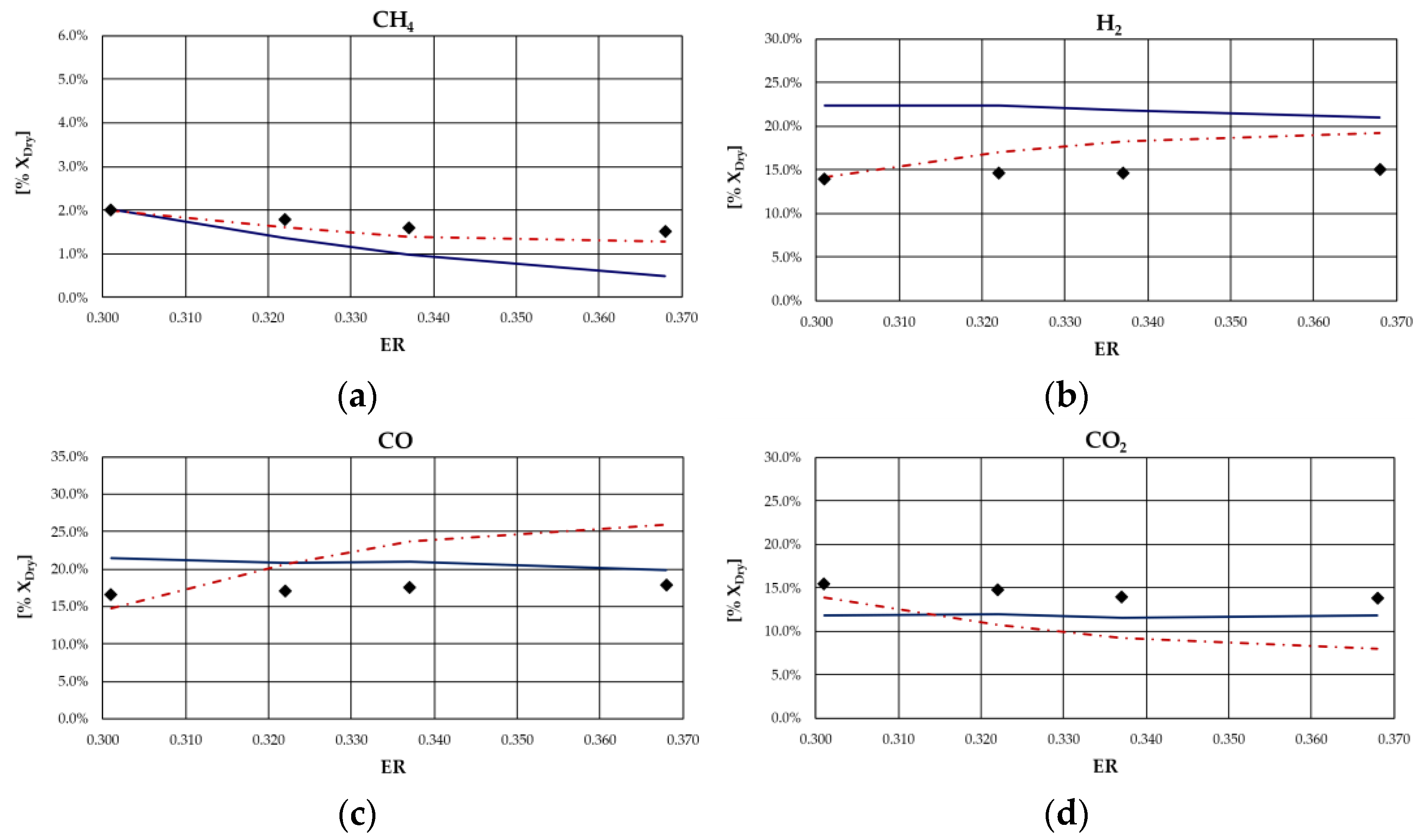
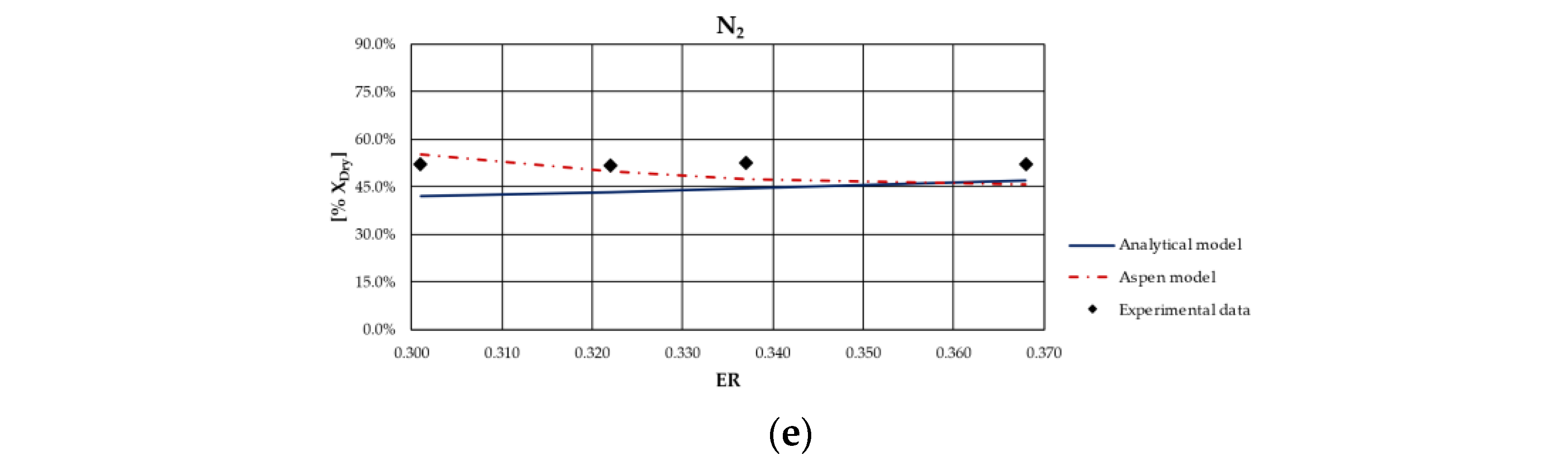
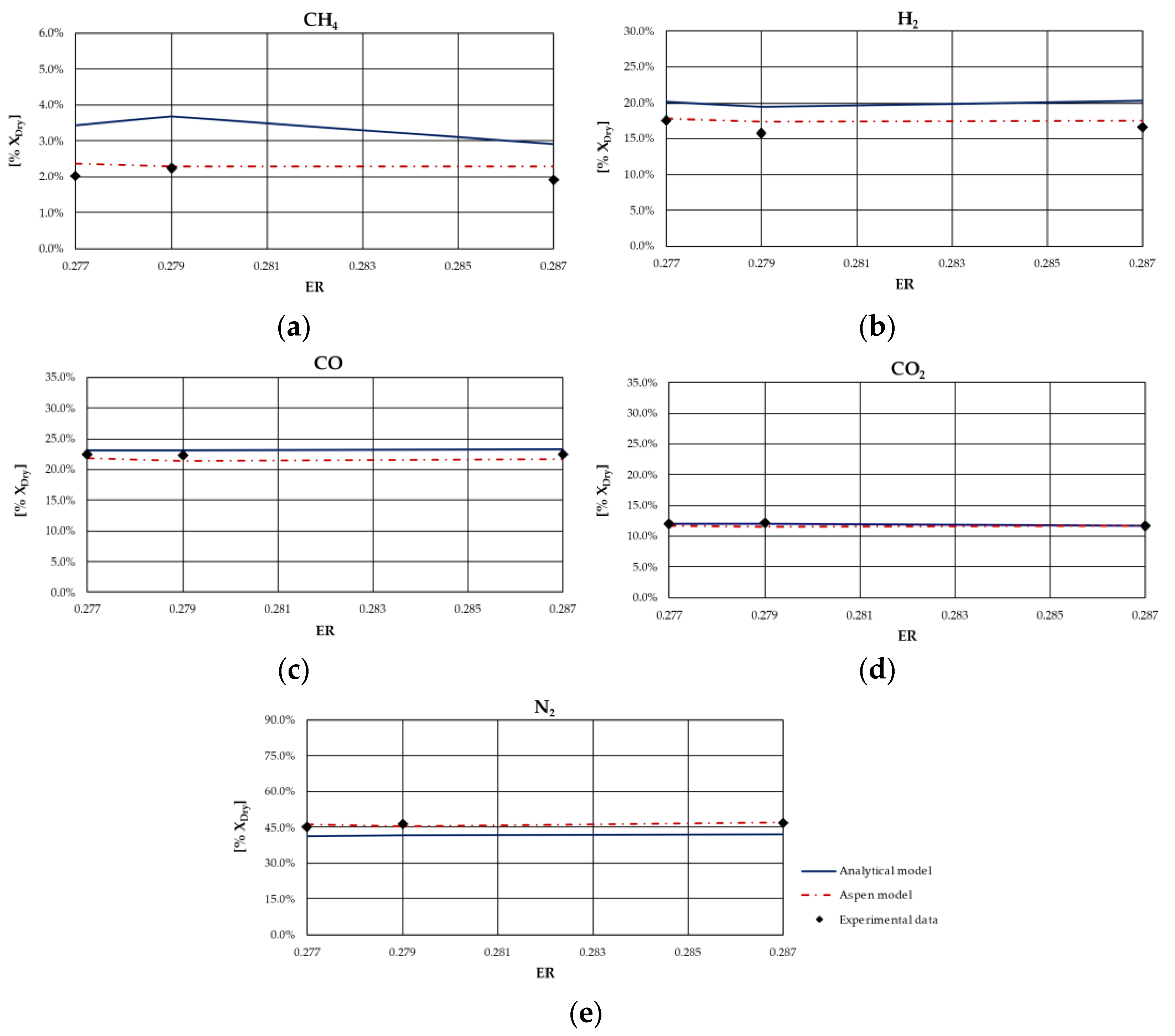
2 content tended to be underestimated by the analytical model for each simulated case, probably because of the restrictive hypothesis of complete carbon conversion on which the model is based. Regarding the Aspen model, a generally satisfactory agreement between the numerical results and the experimental data could be observed, except for the experiments carried out in [
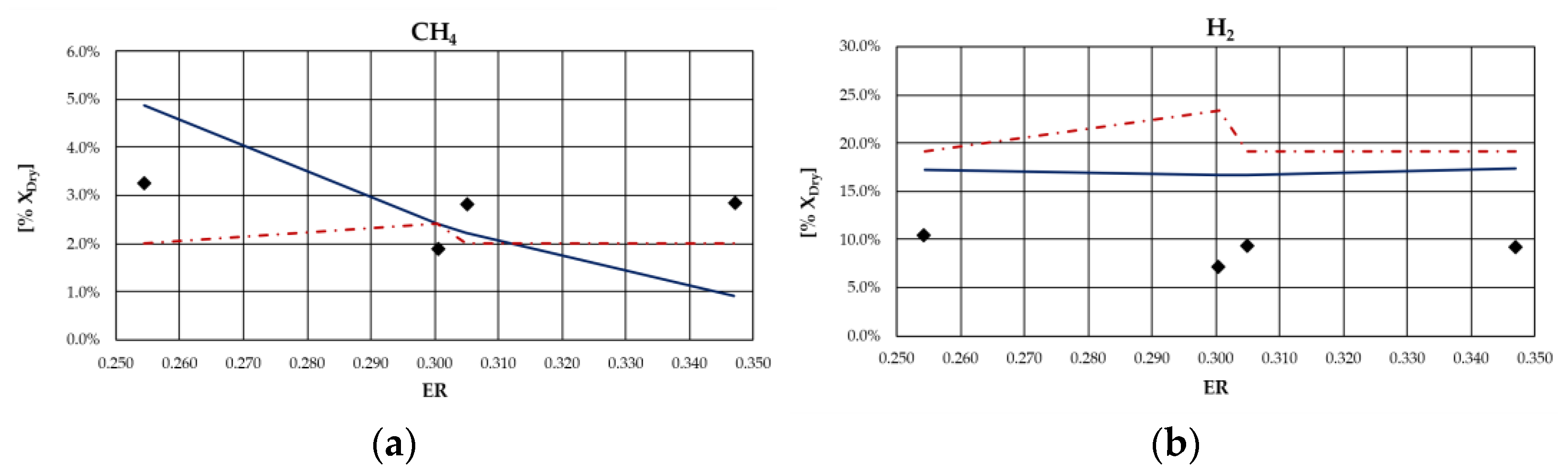
68] for which the trend of the fuel compounds, CH
4 and H
2, was not adequately captured. Ignoring this last group of results, the highest average deviation between the numerical and the experimental data was 23%, obtained for the first case of the experiment carried out in [
66]. Specifically, the concentration of CH
4, which slightly decreased with ER, was well predicted by the model. Such a result is promising since usually the compounds characterized by the lowest concentrations, such as methane, are the ones yielding the highest deviations between numerical and experimental results. In addition, the trend of H
2 concentration, which slightly varies with ER, was fairly predicted by the model, except for the experiment carried out in [
67] and shown
Figure 4. This could be related to the variation in moisture content that influences H
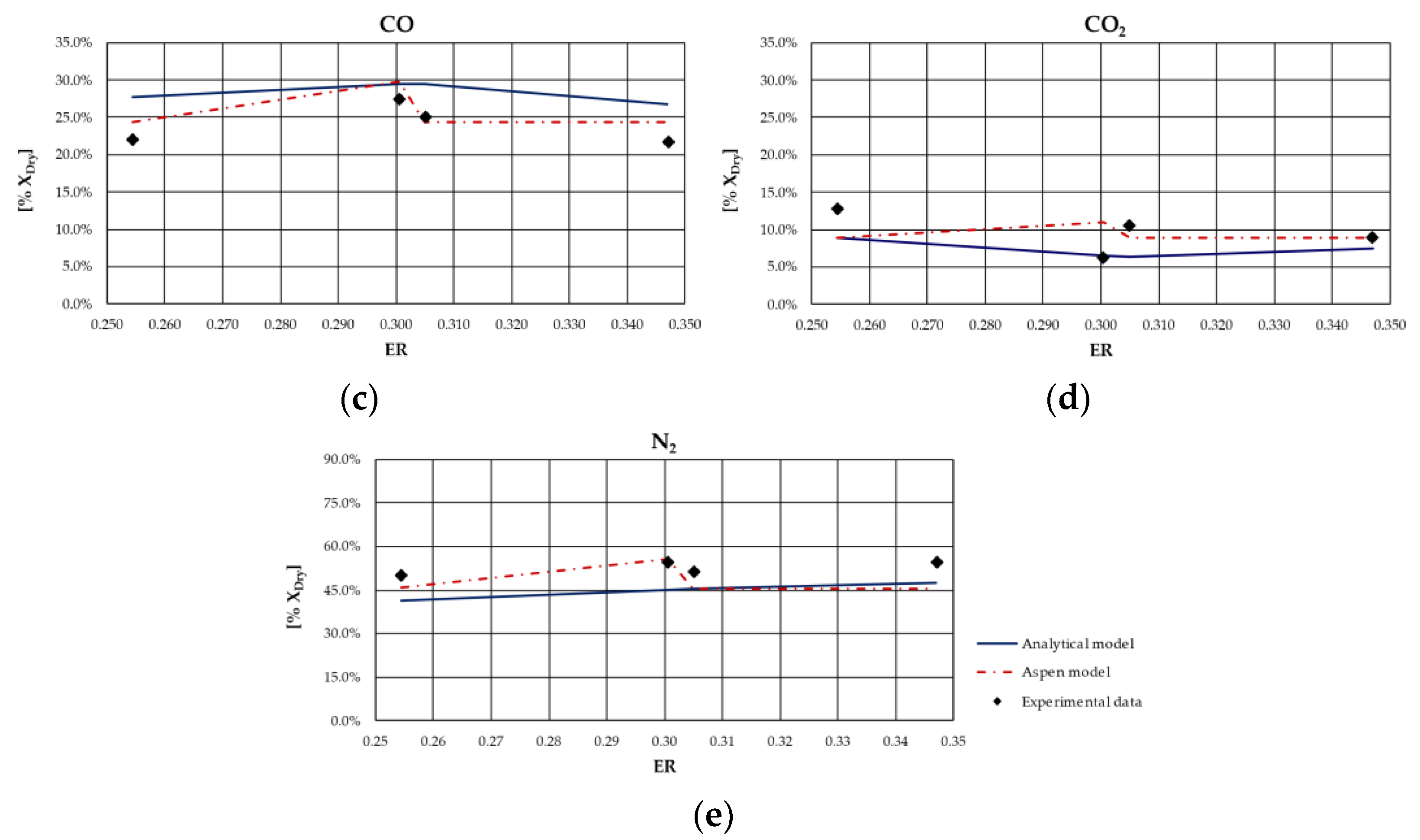
2 concentration in the syngas. The concentrations of CO and CO
2 usually showed an inverse trend due to the water shift reaction in which they are involved. Their trend, as well as that of N
2, was in excellent agreement with the experimental results. Obviously, the higher the ER, the higher the dilution and thus the N
2 concentration.
As expected, the obtained results evidenced that the major limitation of both models lies in the thermodynamic equilibrium assumption and in neglecting tar and char. In fact, the results showed that syngas composition is better reproduced for biomass types characterized by a low ash content and consequently a relatively high heating value. Indeed, the major deviations from experimental data were obtained for the case of gasification of rice husks, whose ash content is approximately 16.6% on a dry basis, as can be noted in
Figure 7. This can be ascribed to the fact that the model did not simulate the tar and char formation, which in this case were a considerable part of the products of the gasification process.
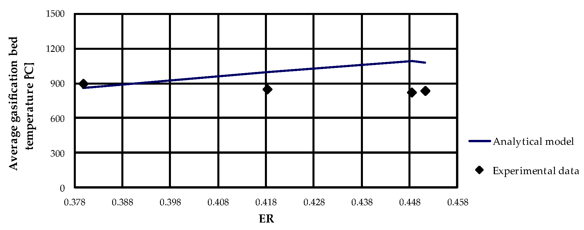
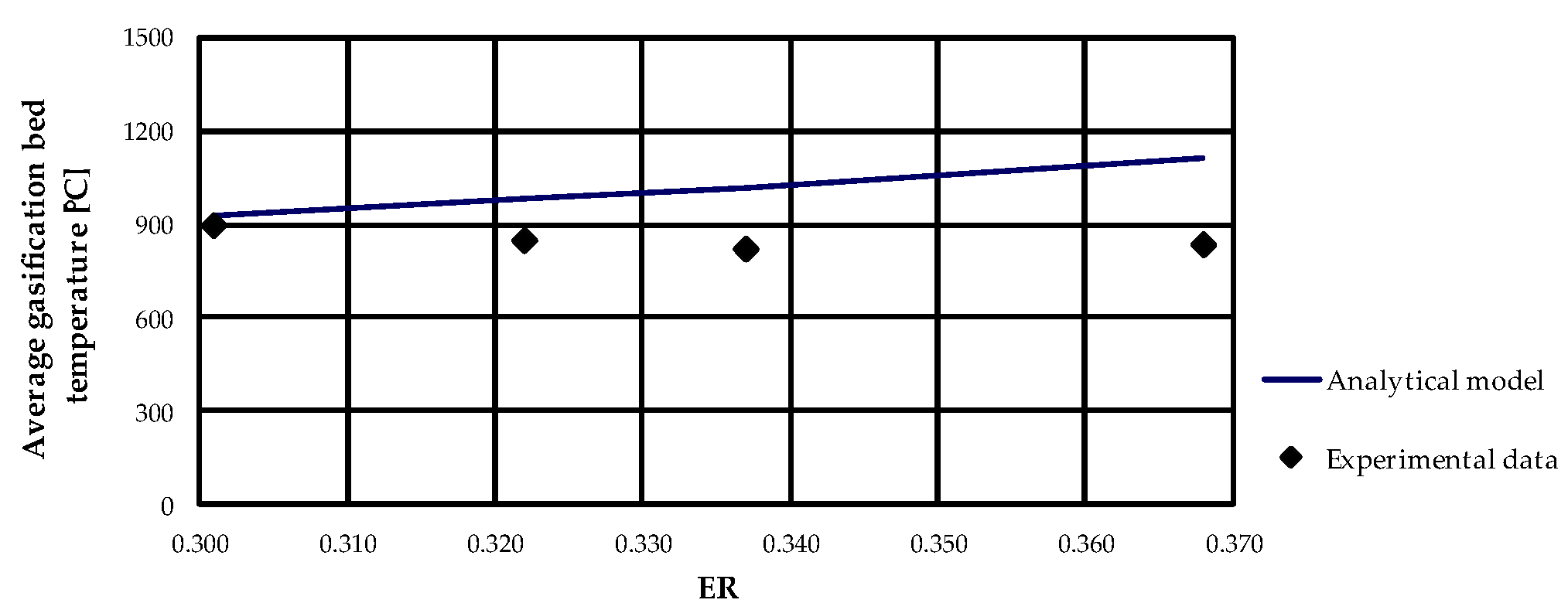
Concerning the evaluation of average gasification bed temperature, as expected, as ER increases the temperature increases, as can be observed from
Figure 3 and
Figure 9. Since the gasifier is assumed to be adiabatic, the analytical model generally overestimated the gasification temperature and the deviation between numerical results and experimental results increased as ER increased.
In general, it can be seen that using a more advanced model of Restricted Equilibrium allows for the obtaining of results closer to experimental ones, minimizing the error between simulated and experimental data, especially for concentrations of CH4 and H2 which, being very low values, are difficult to model. Nevertheless, in the case of the absence of necessary information for calibration, the use of the non-calibrated Aspen model produced non-reliable results. Moreover, it did not predict the gasification temperature. By comparison, the analytical model was more general, and the calibration process allows discovery of the optimal multiplying coefficients of K1 and K2 constants for use as a function of the biomass type and ash content. In addition, the gasification temperature is calculated by solving the energy conservation equation.
In summary, the limit of this approach occurs in critical conditions in which thermodynamic equilibrium is not likely achieved and biomass is characterized by high humidity content, ash, tar and char.
In the future, simulation of tar and char formation will be included in the model. In addition, the model will be implemented in a more complex model of polygeneration systems based on renewable sources, with the aim of optimizing these systems from an energy and economic point of view.
Finally, since the analytical model was based on a non-commercial home-made code, future improvements to better predict methane and hydrogen concentration could be easily implemented.
5. Conclusions
In this paper, the reliability of equilibrium gasification models currently available in the scientific literature was investigated to establish whether they can be employed to build new control and optimization schemes and operating maps of biomass gasification systems integrated into polygeneration plants coupled with energy networks. To this aim, the authors developed two thermodynamic equilibrium models using both commercial software (referred as Aspen model) and a simulation tool implemented in a non-commercial script (referred as mathematical model). The developed thermodynamic equilibrium models were applied to different case studies on downdraft gasifiers available in the literature in order to evaluate the accuracy of the simulation results on varying the biomass type and composition and the operating conditions of the gasification process, evidencing the advantages and disadvantages of both models. Obtained results were compared with experimental results in terms of: (i) molar composition of syngas and (ii) average gasification bed temperature.
In general, the simulation results were comparable with the experimental data for both models. Specifically, the results showed that the analytical model predicted syngas composition with better accuracy for biomass types characterized by a low ash content and consequently a relatively high heating value. This can be ascribed to the fact that the model did not simulate tar and char formation. Regarding the Aspen model, it appeared to fairly predict syngas composition at different conditions of ER. However, if the properties of the treated biomass changed, the accuracy of the model might be reduced. Even though CH4 and H2 syngas concentrations are typically very low and difficult to predict, the values predicted by the Aspen model were in satisfactory agreement with experimental results.
Finally, the developed models offer several advantages: (i) do not require details of system geometry or estimation of the necessary time to reach the thermodynamic equilibrium; (ii) employ a limited number of input data; (iii) do not need to employ correlation for the calculation of the biomass gasification temperature. In addition, the adoption of a general model also allows the quick obtaining of results if it is necessary to simulate numerous operating conditions.
In the future, both developed models will be extended by implementing the modeling of char and tar formation. The model will be also implemented in a more complex model of polygeneration systems based on renewable sources to optimize these systems from an energy and economic point of view.
The proposed overview of thermodynamic equilibrium models has significant industrial implications, allowing for selection of the most suitable and reliable model as a function of biomass properties and industrial operating conditions. Therefore, industries will benefit from this work by having a clearer view of the most reliable models for the gasification process.


 ,
, 


