A Smart Energy Recovery System to Avoid Preheating in Gas Grid Pressure Reduction Stations

Abstract

Preheating is often required to prevent hydrate formation during the pressure reduction process in a natural gas distribution network’s pressure reduction station. This paper examines an energy recovery method to avoid the cost and energy consumption of this preheating. The primary aim is to assess the techno-economic feasibility of an energy recovery system based on the Ranque–Hilsch vortex tube coupled to a heat exchanger for large-scale application to the gas grid. To this end, a techno-economic model of the entire energy recovery system was included in an optimisation procedure. The resulting design minimises the payback period (PP) when the system is applied to the pressure reduction stations belonging to a particular gas grid. The pressure reduction stations always operate at an outlet pressure above atmospheric pressure. However, available performance models for the Ranque–Hilsch vortex tube do not permit prediction at backpressure operation. Therefore, a novel empirical model of the device is proposed, and a cost function derived from several manufacturer quotations is introduced for the first time, to evaluate the price of the Ranque–Hilsch vortex tubes. Finally, a nearly complete set of pressure reduction stations belonging to the Italian natural gas grid was chosen as a case study using actual operating parameters collected by each station’s grid manager. The results indicate that the environmental temperature strongly affects the technical and economic feasibility of the proposed energy recovery system. In general, pressure reduction stations operating at an ambient temperature above 0 °C are economically desirable candidates. In addition, the higher the energy recovery system convenience, the higher the flow rate and pressure drop managed by the station. In the Italian case study, 95% of preheating costs could be eliminated with a PP of fewer than 20 years. A 40% preheating cost saving is still possible if the maximum PP is limited to 10 years, and a small but non-negligible 3% of preheating costs could be eliminated with a PP of fewer than 4.5 years.

1. Introduction

In the transition towards a 100% decarbonised energy system, specific actions should be scheduled for each system in the energy supply chain, including energy sources, conversion, transport, storage, and utilisation. Since the progressive substitution of fossil fuel energy sources with renewable ones will require decades, eliminating unnecessary energy consumption could reduce CO₂ emissions in the medium term. Natural gas (NG) will likely be the last fossil fuel abandoned because of its low carbon content and wide availability. Thus, it is worthwhile to pay particular attention to reducing NG consumption, especially in the distribution network. The operating principle of the NG grid is based on controlled pressure drops and corresponding multiple expansions, commonly performed by throttling valves that dissipate the energy previously spent on NG compression. Expansions involve cooling the gas and possible hydrate formation, potentially compromising the integrity of components installed downstream of the pressure reduction stations (PRSs). For this reason, preheating systems consuming NG in boilers are commonly embedded in a PRS. As a result, the operation of the gas grid involves simultaneous dissipations and consumptions of energy, each contributing to CO₂ emissions.

This paper aims to recover energy wasted during gas pressure reduction to avoid the energy consumption imposed by NG preheating and achieve the added benefit of reducing CO₂ emissions. From a thermodynamics viewpoint, the available mechanical energy could be recovered by converting it into work (e.g., expanders) or heat (e.g., dissipative systems). The conversion of pressure energy into work is the most rational thermodynamic process because it wastes the minimum exergy. However, the conversion into work does not eliminate the NG preheating issue, which is exacerbated by the cooling effects of the work extraction. In contrast, energy conversion into heat through dissipation could help in eliminating or reducing the NG preheating issue. Solutions to recover either work or heat from pressure drops have been suggested previously.

Regarding work recovery, radial turbines were proposed several years ago. Still, only a few real applications in which the expansion work has been converted into electricity and either sold to the grid or directly self-consumed in the PRSs have been successful worldwide [1,2,3,4]. As highlighted in [5], the utilisation of radial turbines is generally convenient only in PRSs with unique operating requirements such as very high flow rates and pressure drops. Despite the high efficiency of radial turbines, their high cost cannot be recovered within reasonable periods for small-to-medium size installations. Volumetric expanders may be a less expensive option; however, they have been proposed only in the literature, and no real applications to the NG grid have been realised. The complexity of the entire energy recovery system, the preheating issue, and the regulatory constraints related to the connection to the electric grid discourage gas grid managers from investing in expander-based systems.

On the other hand, thermal energy recovery systems based on dissipation processes have been studied to a limited extent, even though they may overcome the electric connection and preheating issues. Within this category of solutions, Gheselbash et al. [6] very recently proposed adopting a system based on Ranque–Hilsch vortex tubes (RHVTs) coupled to geothermal heat exchangers. The RHVT performs dual actions: It reduces gas pressure and splits the gas flow into two streams having temperatures lower and higher than the inlet temperature, respectively. Accordingly, the authors suggested integrating RHVTs into PRSs to expand NG and deliver the cold stream exiting one side of the device to a geothermal heat exchanger (HE) to absorb heat before merging with the hot stream exiting the other side of the device. As a result, the total flow entering a PRS could be expanded to the desired pressure eliminating, or limiting, the need for gas heating. The authors found that NG preheating could be reduced by approximately 80% even though the very high costs of geothermal HEs undermine the economic feasibility of the system.

Guo et al. [7] presented a similar idea, placing an RHVT downstream of an ejector, followed by a HE that heats the NG, thereby exploiting the environment as a heat source. The expansion of the NG is performed in two stages. The first expansion occurs inside the ejector, fed by the total gas flow rate plus an additional flow rate and recirculated from the hot exit of the HE. The second expansion completes the required NG pressure reduction and occurs inside the RHVT, which delivers its hot exit mass flow fraction to the PRS outlet and its cold exit mass flow fraction to the HE. This system heats the NG exiting the PRS to a temperature above the PRS entering temperature. The authors proved the technical feasibility of the system but did not provide information about costs.

The present paper proposes a system that couples an RHVT with a HE to combine the advantages of the solutions suggested in [6,7] while avoiding their drawbacks. The proposed system removes the ejector (and the need for recirculating an NG fraction) included in the latter solution and substitutes the environment for the geothermal heat source needed by the former. A techno-economic investigation is conducted to determine if the limits imposed by the HE costs can be overcome. In particular, a model of the RHVT-HE recovery system is embedded in an optimisation procedure, searching for the minimum payback period (PP) as a function of the PRS requirements.

This work aims to assess the techno-economic feasibility of the system for large-scale application to an NG grid. Accordingly, this work addresses three significant needs: (i) reliable models capable of predicting the performance of the system components; (ii) realistic cost functions of each system component; (iii) real PRS operating parameters. For item (iii), data collected by NG grid managers on a large sample of PRSs currently installed in Italy were used to analyse the Italian gas grid as a case study. Regarding requirements (i) and (ii), their fulfilment required the availability of a techno-economic model for each system component. Unfortunately, existing mathematical models of the RHVT are not suitable for the current application (as evinced from the brief overview of the RHVT presented in the following sub-section), nor are cost functions accounting for RHVT size available in the literature.

As a result, the first original contribution of this paper is a complete techno-economic model of the RHVT that includes a new empirical model for performance prediction and the first cost function presented in the literature based on quotations provided by manufacturers. The second new contribution concerns the scale of the techno-economic analysis, which extends to the country level and is based on actual Italian gas grid data.

Review of the Literature on the Ranque–Hilsch Vortex Tube

The RHVT was first proposed in 1922 [8], but a general theory of its physics has not been formulated and validated [9]. Currently available models attempt to explain the thermal separation occurring in the RHVT through processes driven by heat transfer, pressure gradients, or entropy generation. Bilga et al. [10] proposed a heat transfer model that also accounts for some geometrical parameters. The authors found up to 37% deviation between predicted and measured thermal separation.

Uday et al. [11] numerically investigated the temperature and pressure distribution inside the RHVT at a specific operating condition. They found good agreement between the thermal separation calculated by computational fluid dynamics (CFDs) and the theoretical predictions of Albhorn et al. [12]. Those theoretical predictions [12] were one of the earlier models to predict the performance of the RHVT, based on the transformation of kinetic energy into heat (with the inclusion of some assumptions derived from experimental data). A study similar to [11] was made by Cockerill [13], who proposed a theoretical heat transfer model valid when the tube length to diameter ratio is in the range of 60–64.

Xue et al. [14] investigated the expansion process governing the thermal separation inside the RHVT, concluding that only an isentropic expansion may occur in the tube, demonstrating the inconsistency of both Joule–Thomson and free expansions. Bruun et al. [15] conducted several experiments attempting to show that the thermal separation performed by the RHVT is mainly due to pressure gradients but found only partial evidence of their hypothesis. Byriuk et al. [16] proposed a mathematical model based on pressure gradients that matches experimental data only if refined using empirical correlations. Kargaran et al. [17] proposed a hybrid theoretical–empirical model to optimise the performance of the RHVT with the second law of thermodynamics considered as its theoretical basis. They found that including entropy generation in the model improves the predictive capability.

Models based on work transfer have only recently been proposed and seem promising, although they have not yet been fully validated. In particular, the model by Polinorov, Liu, and Bej [18,19,20,21] obtained quite good predictions for an extensive range of operating parameters. However, their model requires correction factors for conditions when heat transfer becomes non-negligible.

Attempts to understand the fluid dynamics of the RHVT from experimental data and CFD results can also be found in the literature. Xue et al. [22] provided a general description of the RHVT internal flow by collecting pressure and velocity measurements [23]. They suggest that (i) the flow is expanded and injected tangentially into the annulus of the RHVT; (ii) the rotating fluid moves axially towards the hot exit, while its innermost fraction is progressively retrieved to the cold side of the tube; (iii) while moving towards the hot end, the ‘retrieving’ phenomena is reduced until completely depleted; (iv) hot flow internal recirculations occur from the ‘retrieving’ endpoint to the plug placed at the hot exit of the RHVT. Their findings were confirmed by other CFD studies [24,25,26,27,28].

Several works characterised RHVT performance by experiments with different working fluids or at different operating conditions. Subudhi et al. [29], Sankar et al. [30], Liew et al. [31], and Williams et al. [32] generated performance maps at different inlet pressures and temperatures. Agrawal et al. [33] and Jafargholinejad et al. [34] tested RHVT operation with methane, carbon dioxide, and nitrogen as working fluids at a constant pressure expansion ratio. They found that the temperature separation increases as the adiabatic expansion ratio decreases. The empirical model obtained from experiments by Parker et al. [35] is governed by the expansion ratio because it was found to be the only parameter having predictable effects on RHVT performance.

The influence of RHVT geometry on its performance has also been investigated both numerically and experimentally. Kirmaci et al. [36] and Ylmaz et al. [37] provided a literature review on the most relevant geometrical parameters to RHVT performance. Moraveji et al. [38] numerically investigated the effect on temperature separation and mass flow rate due to the number of inlets, tube length, and diameter of the cold exit section. They found that an increase in the number of inlets allows for a decrease in temperature at the cold and hot sides of the tube, whereas an increased tube length (L) and decreased cold orifice diameter (D) both reduce the mass flow rate. Rafiee et al. [39,40] conducted a numerical and experimental investigation searching for the optimal L/D ratio. They considered three hot and cold RHVT layouts, finding that the best performance was achieved for L/D ratios of 9 (opposite direction of the flows), 10 (same direction), and 11 (opposite direction with additional injection).

Dincer et al. [41] experimentally investigated the effect of the position and diameter of the regulation plug placed at the hot exit of the RHVT. They found that the best performance was obtained using a plug diameter of 5 mm with tip angles of 30° and 60°. Valipour et al. [42] found that tube curvature is always detrimental to RHVT performance. Im et al. [43] performed a parametric study on the effect of injection area and inlet pressure on RHVT performance using experimental data. Mohammadi et al. [44] tested several layouts of tubes having different lengths and nozzle counts. They found that the higher the nozzle count, the smaller the tube length, maximising the temperature differentiations.

Kumar et al. [45] used the Taguchi statistical method to find a design criterion to maximise the outlet temperature at the hot exit, while Bazgir et al. [46] used numerical investigations to find the geometrical parameters to achieve low temperatures at the cold side exit. Cang [47] used available experimental data to find the most promising RHVT design to achieve the performance requested in large flow rate applications. Kormkaz et al. [48] trained an artificial neural network (ANN) with experimental data to generate a performance prediction model that qualitatively predicts the geometrical feature effects on RHVT performance. Thakare et al. [49] provide a comprehensive review of the optimisation criteria proposed in the literature, including those based on ANN.

In summary, many studies have focused on explaining the RHVT working principles while others provide models to predict the device’s performance accounting for different geometrical features. Regardless of the particulars of each work, they all consider RHVT operations expanding the gas to atmospheric pressure. None of them evaluates either the effective costs of the RHVT or its application to actual cases. Thus, none of the existing models can be used to study the application of an RHVT to a PRS.

2. Energy Recovery System Based on RHVT

This section describes the working principle of the proposed energy recovery system with the aid of the sketches provided in Figure 1. Figure 1a summarises the tasks commonly performed by a gas grid PRS to prevent hydrate formation. A boiler burns a fraction of gas to preheat the main gas stream using a heat exchanger upstream of the throttling valve used to reduce pressure. As a result, the gas cooling due to the expansion is controlled (even nullified in the limiting case) to ensure the safe operation of components and monitoring systems installed in the gas line downstream of the PRS.

Figure 1b shows how the same expansion process can be performed by either a standard throttling valve (on the left) or an RHVT (on the right). The equivalent expansion process means the same gas stream cooling and preheating requirements. The system proposed in this paper eliminates the gas consumption for the preheating by exploiting the environment as a thermal source. This is achieved by pairing an RHVT with a finned tube HE and placing this system downstream of the throttling valve (which is still required by the PRS but only as a regulation device), as shown in Figure 1c. In particular, the stream exiting the cold side of the RHVT can absorb heat—via the HE—from the environment before being merged with the hot stream exiting the hot side of the RHVT. Thus, NG exits the PRS at a safe temperature (equal to the pre-expansion temperature in the limiting case), avoiding NG consumption (and corresponding CO2 emissions) and obtaining consistent economic savings.

3. Models and Data

This section deals with the three major requirements of this study as presented at the end of the Introduction Section. These requirements are the RHVT techno-economic models in Section 3.1, the HE in Section 3.2, and the actual gas grid PRS operating data in Section 3.3.

3.1. RHVT Techno-Economic Model

The RHVT techno-economic model is a new empirical sub-model supported by experimental data and the first law of thermodynamics and tailored to performance prediction and provides an economic sub-model to predict the cost of the device. The RHVT model is a ‘black box’ model that expands the gas while splitting the inlet flow into hot and cold streams. Accordingly, this empirical sub-model does not provide additional physical insight into the RHVT, compared with the present state of the art.

The parameters considered as performance indicators include (i) the cooling effect, i.e., the temperature drop $\Delta T_c$; (ii) the heating effect, i.e., the temperature rise $\Delta T_h$; (iii) the mass flow split ratio $x$; (iv) the temperature separation performed by the RHVT, i.e., the temperature separation index $Z$. These performance indicators are defined as follows:

$$\Delta T_c=T_{in}-T_c$$

(1)

$$\Delta T_h=T_h-T_{in}$$

(2)

$$x=\frac{{\dot{m}}_c}{{\dot{m}}_c+{\dot{m}}_h}=\frac{{\dot{m}}_c}{{\dot{m}}_{tot}}$$

(3)

$$Z=\frac{\Delta T_c}{\Delta T_h}$$

(4)

where $T_{in}$ (°C) is the gas inlet temperature, ${\dot{m}}_{tot}$ (kg/s) is the mass flow rate entering the RHVT, and ${\dot{m}}_h$(kg/s) and ${\dot{m}}_c$ (kg/s) are the mass flow rates exiting from the hot and cold sides of the device, respectively.

3.1.1. Prediction of RHVT Performance for Expansion to Ambient Conditions for Gases Other Than Air

The method to estimate the performance for expansions of gases to p = p_amb is derived from the experimental data of [50], which reports experimental measurements of RHVT operation with air as working fluid.

Estimation of the cold-side temperature drop (cooling effect)—the maximum cooling effect $\Delta T_{c,max}$ admitted by an isentropic expansion process depends on the available expansion ratio $r_e$ (-) as follows:

$$\Delta T_{c,max}=T_{in}-T_{is}=T_{in}-f\left(T_{in},p_{in},p_{out}\right)=T_{in}-f\left(T_{in},p_{in},r_e\right)$$

(5)

$$r_e=\frac{p_{in}}{p_{out}}$$

(6)

The cooling efficiency ${\eta }_c$ of the RHVT can be defined as

$${\eta }_c=\frac{\Delta T_{c,exp}}{\Delta T_{c,max}}$$

(7)

where $\Delta T_{c,exp}$ is the experimental temperature drop between the RHVT entrance and the cold side exit as measured during air expansion to ambient pressure at a specified x. When the working fluid is changed from air to a gas with a different specific heat ratio, geometry modifications to the RHVT should be taken into account to achieve high ${\eta }_c$ [42]. However, experimental investigations demonstrate that for a given geometry, the cooling efficiency ${\eta }_c$ seems to be independent of the working fluid type [32]. From this experimental evidence, the cooling effect for an ideal gas other than air for a particular RHVT device expanding to ambient pressure is obtained as the product of $\Delta T_{c,max}$ for the specific working fluid and the ${\eta }_c$ for air at the same r_e. The cold-side performance for methane operation over the entire range of x is reported in

Table A2. Cooling effect and corresponding cooling efficiency for RHVT operation with methane at various expansion and mass flow split ratios.

x	0.2			0.3			0.4			0.5
re	$\Delta {\mathit{T}}_{\mathit{c},\mathit{e}\mathit{x}\mathit{p}}$ $\left[°\mathrm{C}\right]$	$\Delta {\mathit{T}}_{\mathit{c},\mathit{m}\mathit{a}\mathit{x}}$ $\left[°\mathrm{C}\right]$	${\mathit{\eta }}_{\mathit{c}}$	$\Delta {\mathit{T}}_{\mathit{c},\mathit{e}\mathit{x}\mathit{p}}$ $\left[°\mathrm{C}\right]$	$\Delta {\mathit{T}}_{\mathit{c},\mathit{m}\mathit{a}\mathit{x}}$ $\left[°\mathrm{C}\right]$	${\mathit{\eta }}_{\mathit{c}}$	$\Delta {\mathit{T}}_{\mathit{c},\mathit{e}\mathit{x}\mathit{p}}$ $\left[°\mathrm{C}\right]$	$\Delta {\mathit{T}}_{\mathit{c},\mathit{m}\mathit{a}\mathit{x}}$ $\left[°\mathrm{C}\right]$	${\mathit{\eta }}_{\mathit{c}}$	$\Delta {\mathit{T}}_{\mathit{c},\mathit{e}\mathit{x}\mathit{p}}$ $\left[°\mathrm{C}\right]$	$\Delta {\mathit{T}}_{\mathit{c},\mathit{m}\mathit{a}\mathit{x}}$ $\left[°\mathrm{C}\right]$	${\mathit{\eta }}_{\mathit{c}}$
2.4	29.7	53.4	0.557	28.8	53.4	0.539	26.9	53.4	0.504	24.5	53.4	0.458
3	35.6	65.5	0.544	34.5	65.5	0.527	32.3	65.5	0.493	29.4	65.5	0.449
4	44.3	80.3	0.552	42.8	80.3	0.533	40.2	80.3	0.501	36.6	80.3	0.456
5	50.4	91.1	0.553	48.4	91.1	0.531	45.0	91.1	0.494	40.8	91.1	0.448
6	54.8	99.6	0.550	52.5	99.6	0.527	48.8	99.6	0.490	44.0	99.6	0.441
7	58.4	106.5	0.549	56.0	106.5	0.526	52.0	106.5	0.488	47.1	106.5	0.442
8	61.5	112.2	0.548	59.0	112.2	0.526	55.0	112.2	0.490	49.9	112.2	0.445
9	64.0	117.2	0.546	61.3	117.2	0.523	57.4	117.2	0.490	51.5	117.2	0.440
	0.6			0.7			0.8
2.4	21.1	53.4	0.395	17.3	53.4	0.324	13.5	53.4	0.253
3	25.4	65.5	0.388	20.9	65.5	0.319	15.8	65.5	0.241
4	31.7	80.3	0.394	26.1	80.3	0.325	19.3	80.3	0.240
5	35.4	91.1	0.389	29.1	91.1	0.320	22.2	91.1	0.244
6	38.3	99.6	0.384	31.9	99.6	0.320	23.9	99.6	0.240
7	40.7	106.5	0.383	33.6	106.5	0.315	25.6	106.5	0.240
8	43.0	112.2	0.383	35.5	112.2	0.316	26.9	112.2	0.240
9	45.0	117.2	0.384	36.7	117.2	0.313	27.3	117.2	0.233

in Appendix A (the corresponding data derived from measurements [50] in air operation are reported in

Table A1. Experimental cooling effect and corresponding cooling efficiency for RHVT operation with air at various expansion and mass flow split ratios (data from [50]).

x	0.2			0.3			0.4			0.5
re	$\Delta {\mathit{T}}_{\mathit{c},\mathit{e}\mathit{x}\mathit{p}}$ $\left[°\mathrm{C}\right]$	$\Delta {\mathit{T}}_{\mathit{c},\mathit{m}\mathit{a}\mathit{x}}$ $\left[°\mathrm{C}\right]$	${\mathit{\eta }}_{\mathit{c}}$	$\Delta {\mathit{T}}_{\mathit{c},\mathit{e}\mathit{x}\mathit{p}}$ $\left[°\mathrm{C}\right]$	$\Delta {\mathit{T}}_{\mathit{c},\mathit{m}\mathit{a}\mathit{x}}$ $\left[°\mathrm{C}\right]$	${\mathit{\eta }}_{\mathit{c}}$	$\Delta {\mathit{T}}_{\mathit{c},\mathit{e}\mathit{x}\mathit{p}}$ $\left[°\mathrm{C}\right]$	$\Delta {\mathit{T}}_{\mathit{c},\mathit{m}\mathit{a}\mathit{x}}$ $\left[°\mathrm{C}\right]$	${\mathit{\eta }}_{\mathit{c}}$	$\Delta {\mathit{T}}_{\mathit{c},\mathit{e}\mathit{x}\mathit{p}}$ $\left[°\mathrm{C}\right]$	$\Delta {\mathit{T}}_{\mathit{c},\mathit{m}\mathit{a}\mathit{x}}$ $\left[°\mathrm{C}\right]$	${\mathit{\eta }}_{\mathit{c}}$
2.4	34.4	61.7	0.557	33.3	61.7	0.539	31.1	61.7	0.504	28.3	61.7	0.458
3	40.9	75.2	0.544	39.6	75.2	0.527	37.1	75.2	0.493	33.8	75.2	0.449
4	50.4	91.3	0.552	48.7	91.3	0.533	45.7	91.3	0.501	41.6	91.3	0.456
5	56.9	103.0	0.553	54.7	103.0	0.531	50.9	103.0	0.494	46.1	103.0	0.448
6	61.6	111.9	0.550	59	111.9	0.527	54.8	111.9	0.490	49.4	111.9	0.441
7	65.4	119.2	0.549	62.7	119.2	0.526	58.2	119.2	0.488	52.7	119.2	0.442
8	68.6	125.2	0.548	65.8	125.2	0.526	61.4	125.2	0.490	55.7	125.2	0.445
9	71.1	130.3	0.546	68.2	130.3	0.523	63.8	130.3	0.490	57.3	130.3	0.440
	0.6			0.7			0.8
2.4	24.4	61.7	0.395	20	61.7	0.324	15.6	61.7	0.253
3	29.2	75.2	0.388	24	75.2	0.319	18.1	75.2	0.241
4	36	91.3	0.394	29.7	91.3	0.325	21.9	91.3	0.240
5	40	103.0	0.389	32.9	103.0	0.320	25.1	103.0	0.244
6	43	111.9	0.384	35.8	111.9	0.320	26.9	111.9	0.240
7	45.6	119.2	0.383	37.6	119.2	0.315	28.6	119.2	0.240
8	48	125.2	0.383	39.6	125.2	0.316	30	125.2	0.240
9	50	130.3	0.384	40.8	130.3	0.313	30.4	130.3	0.233

).

Estimation of the hot-side temperature rise (heating effect)—assuming that the RHVT walls are adiabatic, from energy conservation across the RHVT control volume, the maximum heating effect (temperature rise) of an ideal gas on the hot side of the RHVT can be estimated from

$${\dot{m}}_{tot}·x·\left(h_{in}-h_c\right)={\dot{m}}_{tot}·\left(1-x\right)·\left(h_{in}-h_{h,max}\right)$$

(8)

$$h_{h,max}=h_{in}-\frac{x·\left(h_{in}-h_c\right)}{\left(1-x\right)}$$

(9)

$$\Delta T_{h,max}=T_{h,max}-T_{in}=T\left(h_{h,max},p_{out}\right)-T_{in}$$

(10)

For each $x$, the heating efficiency of the RHVT can be defined as

$${\eta }_h=\frac{\Delta T_{h,exp}}{\Delta T_{h,max}}$$

(11)

where $\Delta T_{h,exp}$ is the experimental temperature rise between the RHVT entrance and the hot side exit as measured during air expansion to ambient pressure. As for the cooling effect, the heating effect for methane operation can be predicted by calculating the $\Delta T_{h,max}$ using Equations (8)–(10) and assuming the heating efficiencies ${\eta }_h$ obtained for air operation.

Table A4. Heating effect, heating efficiency, and index Z for RHVT operation with methane at various expansion and mass flow split ratios.

x	0.2				0.3				0.4				0.5
re	$\Delta {\mathit{T}}_{\mathit{h},\mathit{e}\mathit{x}\mathit{p}}$ [°C]	$\Delta {\mathit{T}}_{\mathit{h},\mathit{m}\mathit{a}\mathit{x}}$ [°C]	${\mathit{\eta }}_{\mathit{h}}$	$\mathit{Z}$	$\Delta {\mathit{T}}_{\mathit{h},\mathit{e}\mathit{x}\mathit{p}}$ [°C]	$\Delta {\mathit{T}}_{\mathit{h},\mathit{m}\mathit{a}\mathit{x}}$ [°C]	${\mathit{\eta }}_{\mathit{h}}$	$\mathit{Z}$	$\Delta {\mathit{T}}_{\mathit{h},\mathit{e}\mathit{x}\mathit{p}}$ [°C]	$\Delta {\mathit{T}}_{\mathit{h},\mathit{m}\mathit{a}\mathit{x}}$ [°C]	${\mathit{\eta }}_{\mathit{h}}$	$\mathit{Z}$	$\Delta {\mathit{T}}_{\mathit{h},\mathit{e}\mathit{x}\mathit{p}}$ [°C]	$\Delta {\mathit{T}}_{\mathit{h},\mathit{m}\mathit{a}\mathit{x}}$ [°C]	${\mathit{\eta }}_{\mathit{h}}$	$\mathit{Z}$
2.4	6.7	7.0	0.953	4.4	11.4	12.0	0.954	2.5	16.6	17.5	0.944	1.6	23.5	24.0	0.978	1.0
3	7.8	8.3	0.946	4.6	13.4	14.2	0.943	2.6	19.8	20.8	0.949	1.6	27.5	28.6	0.962	1.1
4	9.4	9.6	0.979	4.7	16.1	16.7	0.963	2.7	24.2	24.6	0.982	1.7	33.1	33.8	0.977	1.1
5	10.1	10.4	0.976	5.0	17.5	18.3	0.955	2.8	26.3	27.2	0.967	1.7	35.8	37.4	0.956	1.1
6	10.3	10.9	0.949	5.3	18.4	19.4	0.948	2.9	27.5	28.9	0.950	1.8	37.6	39.9	0.942	1.2
7	10.4	11.2	0.933	5.6	19.0	20.2	0.940	3.0	28.5	30.2	0.944	1.8	39.0	41.8	0.933	1.2
8	10.4	11.3	0.923	5.9	19.4	20.7	0.935	3.0	29.5	31.2	0.945	1.9	40.0	43.2	0.926	1.2
9	10.2	11.3	0.900	6.3	19.4	21.1	0.919	3.2	29.8	31.9	0.936	1.9	40.9	44.3	0.925	1.3
	0.6				0.7				0.8
2.4	29.5	31.2	0.947	0.7	38.0	39.7	0.958	0.5	47.9	50.1	0.956	0.3
3	35.2	37.1	0.948	0.68	44.8	47.2	0.950	0.5	56.4	60.2	0.936	0.3
4	42.8	43.9	0.976	0.69	54.2	55.8	0.971	0.5	67.0	70.9	0.945	0.3
5	46.4	48.5	0.957	0.70	58.6	61.6	0.951	0.5	72.6	78.1	0.929	0.3
6	49.2	51.8	0.949	0.71	61.9	65.7	0.942	0.5	76.5	83.0	0.921	0.3
7	51.2	54.3	0.944	0.71	64.4	68.7	0.937	0.5	79.6	86.6	0.919	0.3
8	52.7	56.1	0.940	0.72	66.4	71.0	0.935	0.5	82.1	89.2	0.920	0.3
9	53.6	57.5	0.933	0.74	67.3	72.7	0.926	0.5	82.5	91.1	0.906	0.3

in Appendix A lists the prediction of the hot-side performance under methane operation (the corresponding data derived from measurements [50] in air operation are reported in

Table A3. Experimental heating effect, heating efficiency, and index Z for RHVT operation with air at various expansion and mass flow split ratios (data from [50]).

x	0.2				0.3				0.4				0.5
re	$\Delta {\mathit{T}}_{\mathit{h},\mathit{e}\mathit{x}\mathit{p}}$ [°C]	$\Delta {\mathit{T}}_{\mathit{h},\mathit{m}\mathit{a}\mathit{x}}$ [°C]	${\mathit{\eta }}_{\mathit{h}}$	$\mathit{Z}$	$\Delta {\mathit{T}}_{\mathit{h},\mathit{e}\mathit{x}\mathit{p}}$ [°C]	$\Delta {\mathit{T}}_{\mathit{h},\mathit{m}\mathit{a}\mathit{x}}$ [°C]	${\mathit{\eta }}_{\mathit{h}}$	$\mathit{Z}$	$\Delta {\mathit{T}}_{\mathit{h},\mathit{e}\mathit{x}\mathit{p}}$ [°C]	$\Delta {\mathit{T}}_{\mathit{h},\mathit{m}\mathit{a}\mathit{x}}$ [°C]	${\mathit{\eta }}_{\mathit{h}}$	$\mathit{Z}$	$\Delta {\mathit{T}}_{\mathit{h},\mathit{e}\mathit{x}\mathit{p}}$ [°C]	$\Delta {\mathit{T}}_{\mathit{h},\mathit{m}\mathit{a}\mathit{x}}$ [°C]	${\mathit{\eta }}_{\mathit{h}}$	$\mathit{Z}$
2.4	8.3	8.7	0.953	4.1	13.9	14.6	0.954	2.4	20.0	21.2	0.944	1.5	28.3	29.0	0.978	1
3	9.8	10.4	0.946	4.2	16.4	17.4	0.943	2.4	24.0	25.3	0.949	1.5	33.3	34.6	0.962	1
4	12.0	12.3	0.979	4.2	19.9	20.7	0.963	2.4	29.6	30.1	0.982	1.5	40.3	41.3	0.977	1
5	13.2	13.5	0.976	4.3	21.9	22.9	0.955	2.5	32.4	33.5	0.967	1.6	43.9	45.9	0.956	1
6	13.7	14.4	0.949	4.5	23.3	24.6	0.948	2.5	34.2	36.0	0.950	1.6	46.5	49.4	0.942	1.1
7	14.1	15.1	0.933	4.6	24.3	25.9	0.940	2.6	35.8	37.9	0.944	1.6	48.6	52.1	0.933	1.1
8	14.4	15.6	0.923	4.8	25.1	26.8	0.935	2.6	37.3	39.5	0.945	1.6	50.2	54.2	0.926	1.1
9	14.4	16.0	0.900	4.9	25.4	27.6	0.919	2.7	38.1	40.7	0.936	1.7	51.8	56.0	0.925	1.1
	0.6				0.7				0.8
2.4	35.6	37.6	0.947	0.68	46.1	48.1	0.958	0.43	59.4	62.2	0.956	0.26
3	42.6	45.0	0.948	0.68	54.6	57.5	0.950	0.44	69.5	74.2	0.936	0.26
4	52.3	53.6	0.976	0.69	66.5	68.5	0.971	0.45	83.5	88.4	0.945	0.26
5	57.1	59.7	0.957	0.70	72.5	76.2	0.951	0.45	91.2	98.2	0.929	0.27
6	60.9	64.2	0.949	0.71	77.2	82.0	0.942	0.46	97.1	105.4	0.921	0.28
7	63.9	67.7	0.944	0.71	81.0	86.5	0.937	0.46	102.1	111.1	0.919	0.28
8	66.3	70.5	0.940	0.72	84.2	90.0	0.935	0.47	106.3	115.5	0.920	0.28
9	67.9	72.8	0.933	0.74	86.1	93.0	0.926	0.47	107.9	119.1	0.906	0.28

).

The performance data derived from the experiments for air operation and predicted for methane operation are summarised in Figure 2, which shows the cooling and heating effects against $r_e$ for a range of $x$ (0.2–0.8).

3.1.2. Prediction of RHVT Performance for Gas Expansion to Any Backpressure

The literature has never considered generalising the RHVT performance prediction for expansions to a pressure level above atmospheric pressure. The empirical method proposed here is based on the assumption that the temperature separation index Z depends on the mass flow split ratio $x$ alone for a given r_e value. This assumption is supported by Figure 3a, obtained from the experimental data reported in Table A3, where the very slight dependence of Z on r_e is apparent for x > 0.2. The same observation applies to the heating and cooling efficiencies, as shown in Figure 3b. As a result, for a given r_e, there is a value of $x$ corresponding to a triad of values (h_h, h_c, Z) collected in Table A1 and Table A3, regardless of the backpressure level.

The method to calculate RHVT performance for p_out > p_amb is summarised in the flow-chart in Figure 4 and described as follows: First, the performance chart for expansion to atmospheric pressure is derived for the actual working fluid (e.g., the bottom chart in Figure 2 for methane). This is accomplished using the experimental data for air expansions (top chart in Figure 2) according to the procedure described in the previous sub-section. Then, given the RHVT entrance conditions, the specific backpressure p_out > p_amb and the corresponding r_e and $\Delta T_{c,max}$ are calculated using Equation (5). The value of x required to completely define the RHVT operation corresponds to the only triad (h_h, h_c, Z) in Figure 3 that satisfies Equation (8) with the values of the performance parameters $\Delta T_c$, $\Delta T_h$, and $\Delta T_{h,max}$ calculated using Equations (4), (7) and (11), respectively.

3.1.3. Validation of the RHVT Performance Sub-Model

This empirical model allows the RHVT performance to be evaluated at any operating condition with any working fluid. Only a few experimental data are available in the literature for RHVT operation with p_out > p_amb. The black markers and corresponding approximation curves in Figure 5a (taken from [32]) show RHVT experimental data for air and methane expanded to p_out > p_amb. The red and green dots in the figure indicate the performance parameters predicted by the method presented above, labelled with letters E and F, which refer to methane expansion from 6 bar to 1.5 and 2 bar, respectively. Figure 5b superimposes the predictions of the model (red dots) on the experimental curve provided by [51] for RHVT expansion of air from 7.9 bar to 1.7 bar. A good agreement between predictions and experimental data is apparent.

3.1.4. RHVT Cost Function

The cost function was derived from a large number of quotations provided by RHVT manufacturers. This cost function accounts for all investment costs, including on-site installation costs. To a first approximation, RHVT operating and maintenance (O&M) costs are neglected because they are reasonably low, compared with the initial investment, since they do not perform combustion processes or include moving parts or electronics.

It was found that the RHVT cost ($C_{RHVT}$) depends linearly on the inlet volume flow rate (${\dot{V}}_{in}$) according to the following equation:

$$C_{RHVT}=\mathrm{331,953}·{\dot{V}}_{in}\left[EUR\right]$$

(12)

It is worth noting that for a given standard volume flow rate, ${\dot{V}}_{in}$, the RHVT cost depends on the inlet pressure. For example, Figure 6 shows the RHVT cost against the inlet pressure for a standard volume flow rate equal to 100,000 Sm³/h.

3.2. HE Techno-Economic Model

The finned tube HE heats the cold stream exiting the RHVT using the environment as a heat source. The ambient air on the shell side is kept in motion only by natural convection to avoid additional energy consumption by fans. The heat transfer (thermal power) $Q$ (W) can be calculated as follows:

$$Q=K·A·\Delta T_{ml}·F_t$$

(13)

where $K$ (W/m²K) is the global heat exchange coefficient, $A$ (m²) is heat transfer area, $\Delta T_{ml}$ (K) is the logarithmic mean temperature difference, and $F_t$ (-) is a correction factor (taken equal to 1). Following the suggestions of manufacturers, the HE performance is computed by fixing $K=10\mathrm{W}/{\mathrm{m}}^2\mathrm{K}$ and calculating $\Delta T_{ml}$ as follows:

$$\Delta T_{ml}=\frac{\left(\frac{(T_{amb}+T_{c,in})}{2}-T_{c,in}\right)-\left(T_{amb}-T_{c,out}\right)}{ln\left(\frac{\frac{(T_{amb}+T_{c,in})}{2}-T_{c,in}}{T_{amb}-T_{c,out}}\right)}$$

(14)

where $T_{amb}$ (K) is the ambient temperature while $T_{c,in}$ (K) and $T_{c,out}$ (K) are the cold gas inlet and outlet temperatures. According to Equation (14), the temperature difference on the cold side of the HE is calculated using the average of $T_{amb}$ and $T_{c,in}$ (Figure 7) as the temperature of the air exiting the HE, rather than $T_{amb}$. This assumption leads to a larger heat exchange surface A. This apparent oversizing has been included in the model to account in a simple way (consistent with the paper’s goal) for the decrease in HE performance due to icing of its cold surface and natural convection on the shell side. The absence of forced air circulation involves an increasing air temperature profile from the HE entrance to the exit.

The minimum allowed temperature difference $\Delta T_{min}$ between the hot and cold fluids is set equal to 7 °C.

HE Cost Function

As for the RHVT cost function, the HE cost function was derived from manufacturers’ quotations, taking into account the total investment cost, including on-site installation, and neglecting O&M costs. Although the absence of combustion processes, moving parts, and electronics supports ignoring O&M costs for an HE, the cleaning operation is generally a non-negligible maintenance cost. However, the oversized heat exchange surface discussed in the previous sub-section justifies neglecting the cleaning costs. Figure 8 shows the cost function associated with the heat exchanger.

3.3. Data from PRSs of the Italian Gas Grid

To study the proposed energy recovery system design and evaluate its techno-economic feasibility for a given PRS, the availability of the actual annual load curve of the PRS is mandatory. This requirement limits the opportunity to perform a systematic study of all existing PRSs in a gas grid because of the practical difficulty in collecting the annual timesheets for each PRS. A viable alternative is to use data for the mass flow rate processed by a representative station.

For example, in temperate zones, the processed NG mass flow is mainly affected by the seasonality of the consumptions alone. Accordingly, the trend of the NG mass flow rate processed during the year by any PRS belonging to a zonal gas grid is approximately the same. The annual timesheet of the mass flow processed by a representative PRS of the grid can be made dimensionless with respect to the average yearly consumption to obtain a PRS master curve. This PRS master curve can then be used to systematically analyse the proposed energy recovery system embedded in PRSs having different sizes and operating conditions. Data for a specific PRS belonging to the set under analysis can be obtained by simply multiplying the dimensionless trend by its actual average annual consumption.

The PRS master curve used for the present work is shown in Figure 9. This curve was derived from actual data measured in a PRS installed in Padova (northern Italy). This station serves a municipality composed of large urban and industrial areas, so it can be considered to be a reliable example of the annual load distribution of a ‘standard’ PRS.

The curve in Figure 9 was used in conjunction with data made available by the Italian gas grid utility for inlet/outlet pressures and annually averaged mass flow rates processed by the PRSs installed in Italy. Figure 10 shows the cumulative percentage distribution against the processed annually averaged volume flow rate for the 7142 Italian PRSs which require gas preheating. The data show that about 900 out of 7142 (≈13%) of the PRSs process more than 1000 Sm³/h, whereas approximately 80% of the Italian PRSs with preheating systems are relatively small since they process an annual averaged volume flow rate that is less than 500 Sm³/h. This result was largely expected considering that in national gas grids a relatively small number of large PRSs reduces the gas pressure of the entire flow rate consumed in the nation from the maximum level (imposed by the suppliers) to a lower level. On the other hand, many small PRSs are spread all around the country to serve local users with a relatively small flow rate.

4. Methods

This section describes the criteria used to perform the economic evaluations (Section 4.1) and the optimisation procedure used to search for the RHVT–HE energy recovery system design that minimises the PP (Section 4.2).

4.1. Economic Evaluations

The economic evaluations are based on the calculation of the PP. Accordingly, the investment costs and the economic savings derived from eliminating gas consumption for preheating must be determined. The methods employed to calculate the preheating costs and the cost of the proposed energy recovery system are described in what follows.

4.1.1. Calculation of the Preheating Costs

The thermal power $Q_{th}$ (kW) needed for the preheating process is calculated taking into account current legislation (which imposes a temperature of the gas exiting the pressure reduction section $T_{out,ph}$ (K) equal to the temperature at the entrance $T_{in,ph}$), and using the following equations:

$$Q_{th}=\frac{{\dot{m}}_{gas}·\Delta h_{ph}}{{\eta }_{HE}}$$

(15)

$$\Delta h_{ph}=h_{out,ph}-h_{in,ph}=f\left(p_{in},T_{out,ph}\right)-f\left(p_{in},T_{in,ph}\right)$$

(16)

$$h_{out,ph}=h_{out}=f\left(p_{out},T_{in,ph}\right)$$

(17)

where $Q_{th}$ (kW) is the thermal power needed for the preheating process, $\Delta h_{ph}$ (kJ/kg) is the enthalpy increase resulting from preheating, $p_{in}$ and $p_{out}$ (bar) are the inlet and outlet gas pressures, and ${\eta }_{HE}$ is the heat exchanger efficiency (assumed equal to 0.90). Note that $T_{in,ph}$ is dependent on the season.

The annual cost $C_{fuel}$ (EUR) of the NG burned in the boilers for preheating is calculated as

$$C_{fuel}={\displaystyle \sum }_{t=1}^{365}\left(\frac{Q_{th,t}·24\left[h\right]}{{\eta }_B·10.98\left[\frac{kWh}{S{m}^3}\right]}\right)·0.10\left[\frac{EUR}{S{m}^3}\right]$$

(18)

where ${\eta }_B$ is the boiler efficiency, which is set equal to 0.9. Since preheating is imposed only when the pressure drop and the PRS inlet pressure are higher than 12 bar, the expansion of the gas can be performed in a series of stages with and without preheating to minimise the costs. The methodology employed to define the preheating stages is described in the block scheme shown in Figure 11.

Figure 12 shows the preheating cost curves (at yearly constant inlet pressure) obtained for PRSs processing an averaged volume flow rate of 100,000 Sm³/h for multiple combinations of inlet and outlet pressures. For a given inlet pressure, the preheating cost increases as the expansion ratio increases according to a step-like trend, in which each cost step corresponds to an additional preheating stage.

It is interesting to evaluate the preheating costs related to the 7142 PRSs with preheating systems installed in Italy today, whose cumulative percentage number distribution is shown in Figure 10. Figure 13 shows the cumulative percentage distribution of the preheating costs against the processed annually averaged volume flow rate. The curve trend shows that approximately 80% of the preheating costs are due to medium and large-sized PRSs processing volume flow rates above 1000 Sm³/h.

4.1.2. Calculation of the Energy Recovery System Cost

The investment costs of the proposed energy recovery system depend on its size. The size parameters associated with the RHVT and HE are the inlet volume rate $\left({\dot{V}}_{in}\right)$ and surface area ($A$), respectively. The system is sized considering the most demanding PRS conditions, i.e., those maximising the size and costs. These conditions correspond to the maximum flow rate ${\dot{m}}_{in,peak}$ (kg/s) and minimum ambient temperature $T_{amb}$. The inlet volume flow rate ${\dot{V}}_{in}$(m³/s) is calculated as follows:

$${\dot{V}}_{in}=\frac{{\dot{m}}_{in,peak}}{{\rho }_{in}}$$

(19)

$${\rho }_{in}=f\left(p_{in},T_{in}\right)$$

(20)

where ${\rho }_{in}$ (kg/m³) is the gas mass density at the PRS entrance.

The size of the heat exchanger is defined by its exchange surface A (m²), derived from Equations (13) and (14).

$$A=\frac{Q}{K·\Delta T_{ml}·F_t}=\frac{{\dot{m}}_{in,peak}·x·\left(T_{c,out}-T_{c,in}\right)}{K·\Delta T_{ml}·F_t}$$

(21)

The previous equation can be solved once $T_{c,out}$ and $T_{amb}$ are known. The former is found considering that the goal of the process is to avoid gas cooling due to adiabatic expansion (i.e., $T_{in}=T_{out}$). Thus, $T_{c,out}$ can be calculated with the following equations:

$$h_{c,out}=\frac{h_{out}-\left(1-x\right)·h_h}{x}$$

(22)

$$T_{c,out}=f\left(h_{c,out},p_{out}\right)$$

(23)

$$h_{out}=f\left(T_{in},p_{out}\right)$$

(24)

where $h_{out}$ (kJ/kg) is the PRS exit enthalpy after the hot and cold streams are merged, and $h_h$ (kJ/kg) is the enthalpy of the stream exiting the RHVT hot side.

Once the RHVT and HE sizes are known, the cost functions presented in Section 3.1.4 and Section 3.2 allow the cost of the energy recovery system to be calculated.

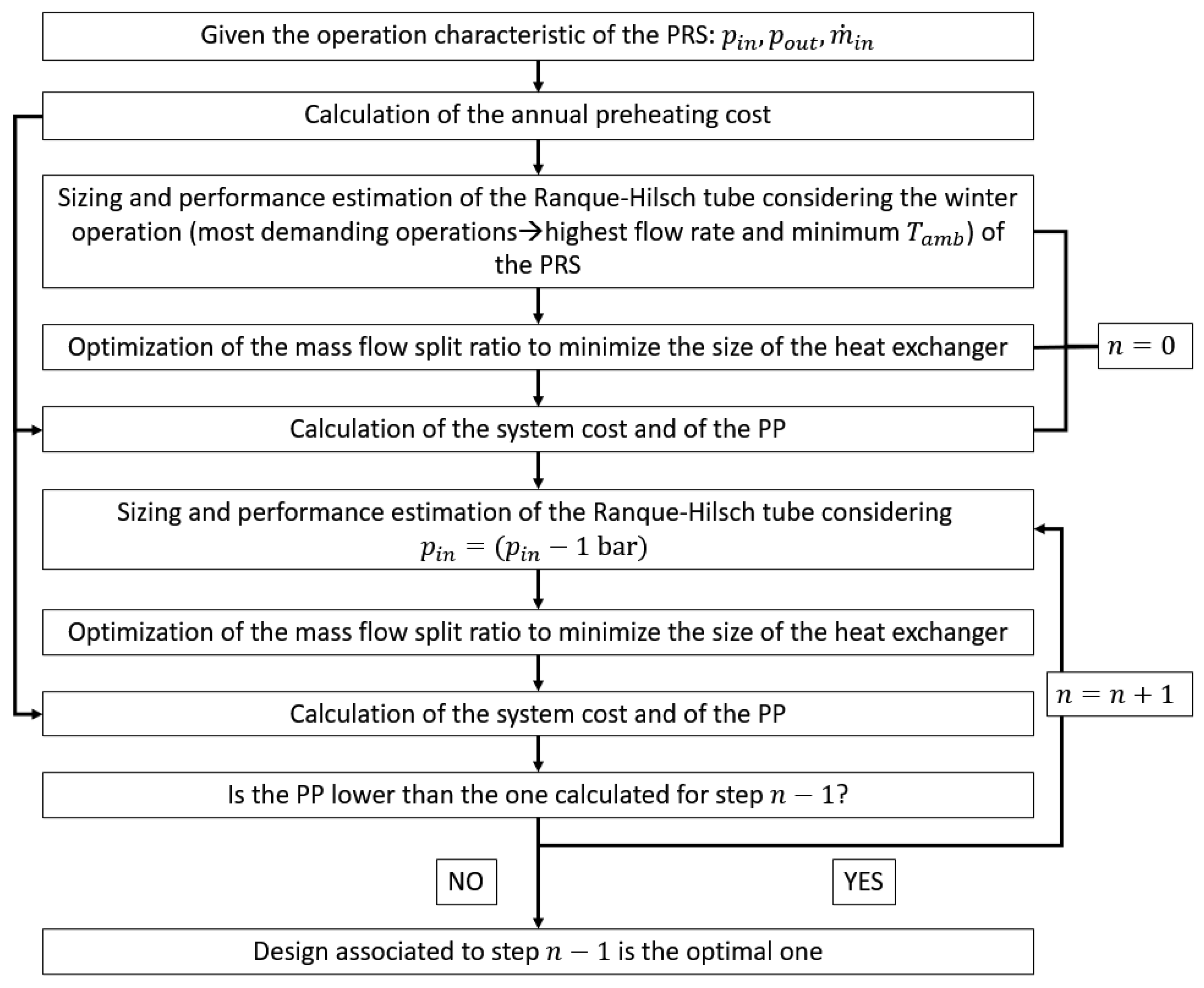
4.2. Design Optimisation Procedure for the RHVT–HE System

The system design criterion minimises the PP with the constraint of achieving an isothermal process between the inlet and the outlet of the pressure reduction section to eliminate the need for preheating. The proposed system can obtain the same NG temperature downstream of the pressure reduction section by several RHVT flow split ratios and inlet pressure combinations. Accordingly, an optimisation is required to find the values that minimise the PP, which is calculated as

$${\displaystyle \sum }_{year=1}^{PP}{F}_{\left(year\right)}·{\left(1+k\right)}^{-year}-F_0=0$$

(25)

where $F_{\left(year\right)}$ is the cash flow in the year being considered, $k$ (=0.015) is the discount rate, and $F_0$ is the investment cost. The cash flow represents the savings derived from not using preheating systems. Figure 14 visualises the optimisation procedure using a flowchart.

The optimisation procedure algorithm was implemented using a visual basic script and the ESS^® software.

5. Application of the Design Optimisation Procedure

The design optimisation procedure just presented was applied in a first example to perform a general investigation of the impact of PRS operating parameters on the proposed energy recovery system’s economic convenience and technical feasibility. In a second example, its economic convenience was evaluated on a real large-scale application.

For the first example, the techno-economic feasibility of the proposed system was investigated considering a 240 PRS sample generated from all possible combinations of inlet pressure, outlet pressure, and annually averaged mass flow rates, listed in

Table 1. Combined operating parameters to generate the general sample.

$p_{in}\left[\mathrm{bar}\right]$	75	70	65	60	55	50	45	40	35	30	25	20
$p_{out}\left[\mathrm{bar}\right]$	60	55	50	45	40	35	30	25	20	15	10	5
${\dot{V}}_{avg}\left[\frac{{\mathrm{Sm}}^3}{\mathrm{h}}\right]$	100	5000	100,000

. This PRS sample resembles a set of PRSs that could be employed by a national gas grid in Europe. The maximum and minimum inlet pressure of the sample (75 bar and 5 bar) were selected according to the common operating ranges of the PRSs, while the three annual averaged volumetric flow rates correspond to three possible stations sizes (small, medium, and large).

The combinations of inlet and outlet pressures characterised by pressure drops below 15 bar were discarded because they did not require preheating. Accordingly, the final sample was reduced to 234 PRSs. The maximum mass flow rate occurring during the year, which is required to size the proposed RHVT–HE energy recovery system, was obtained by multiplying the annual trend gas consumption peak values in Figure 9 by the annual averaged volumetric flow rates from Table 1. According to Figure 9, the largest consumptions of NG occur in January, i.e., during the coldest month of the year in the Northern Hemisphere. In addition, five different ambient temperatures (−10, −5, 0, 5, and 10 °C) were considered since they can strongly vary between different geographical locations belonging to a gas grid.

In the second example application, the optimisation procedure was applied to the entire Italian gas grid as an example of a real case study.

6. Results

The presentation of the results is organised in two sub-sections, each focusing on one of the two example applications described in the previous sub-section.

6.1. Impact of PRS Operating Conditions on the Economic Feasibility of the System

The complete results of this general analysis are provided in Appendix B. A summary of these results, which should assist grid managers in choosing PRSs for which the proposed system is best suited, is given as follows:

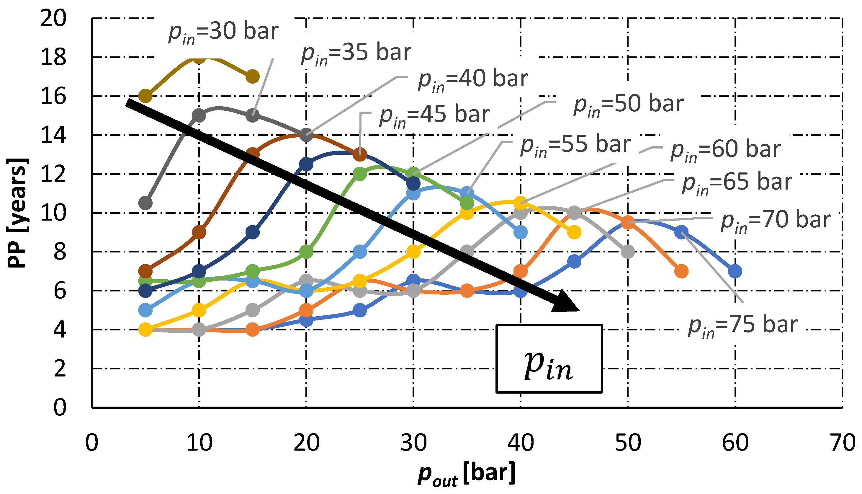
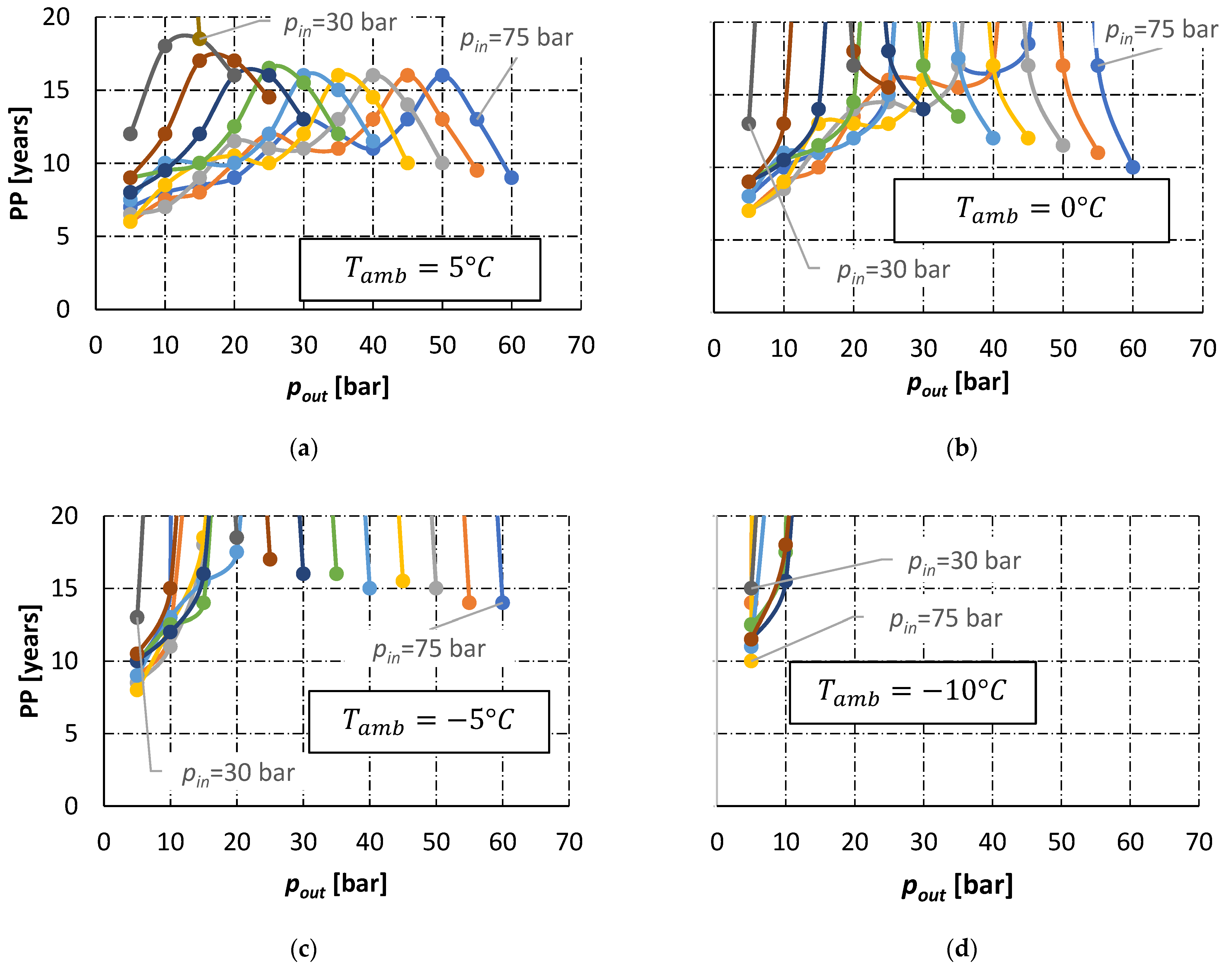
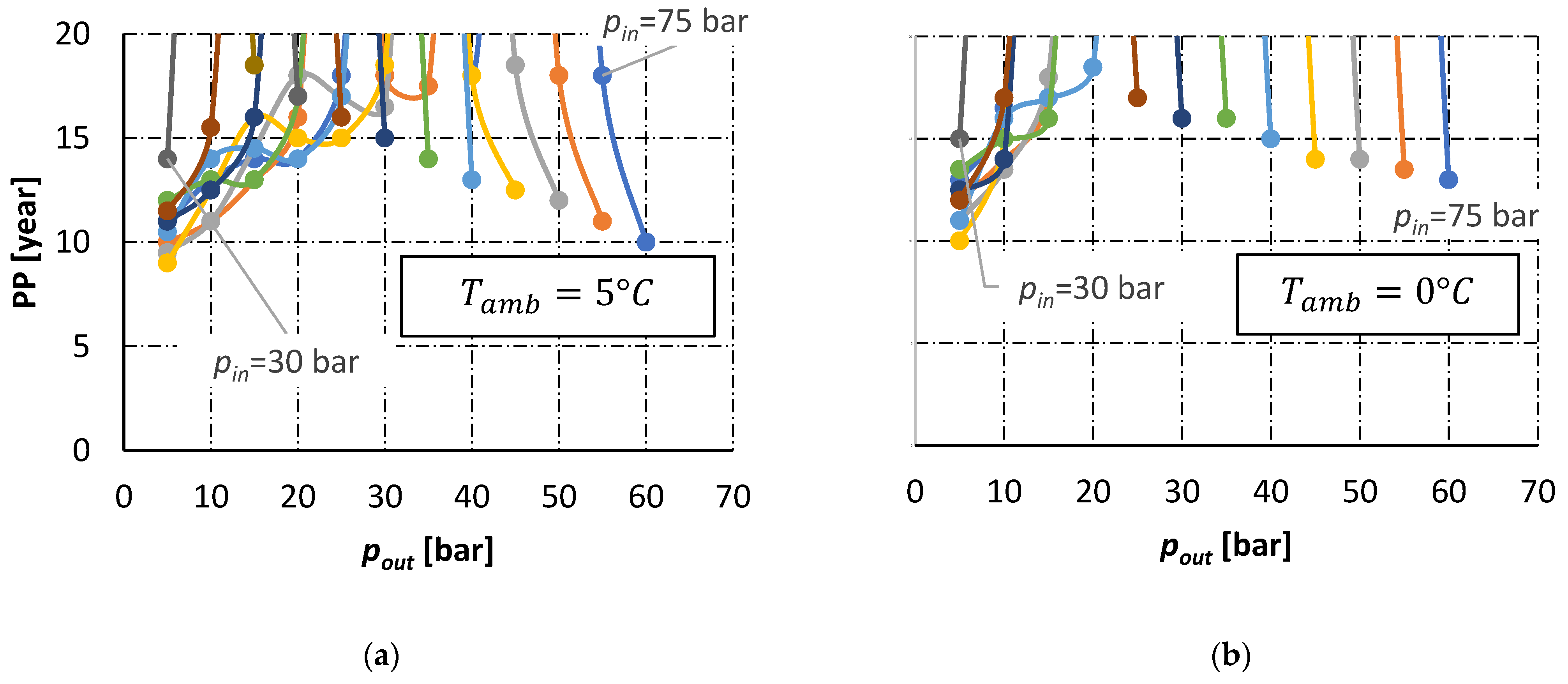
• The PP decreases by increasing the PRS inlet pressure and the expansion ratio;
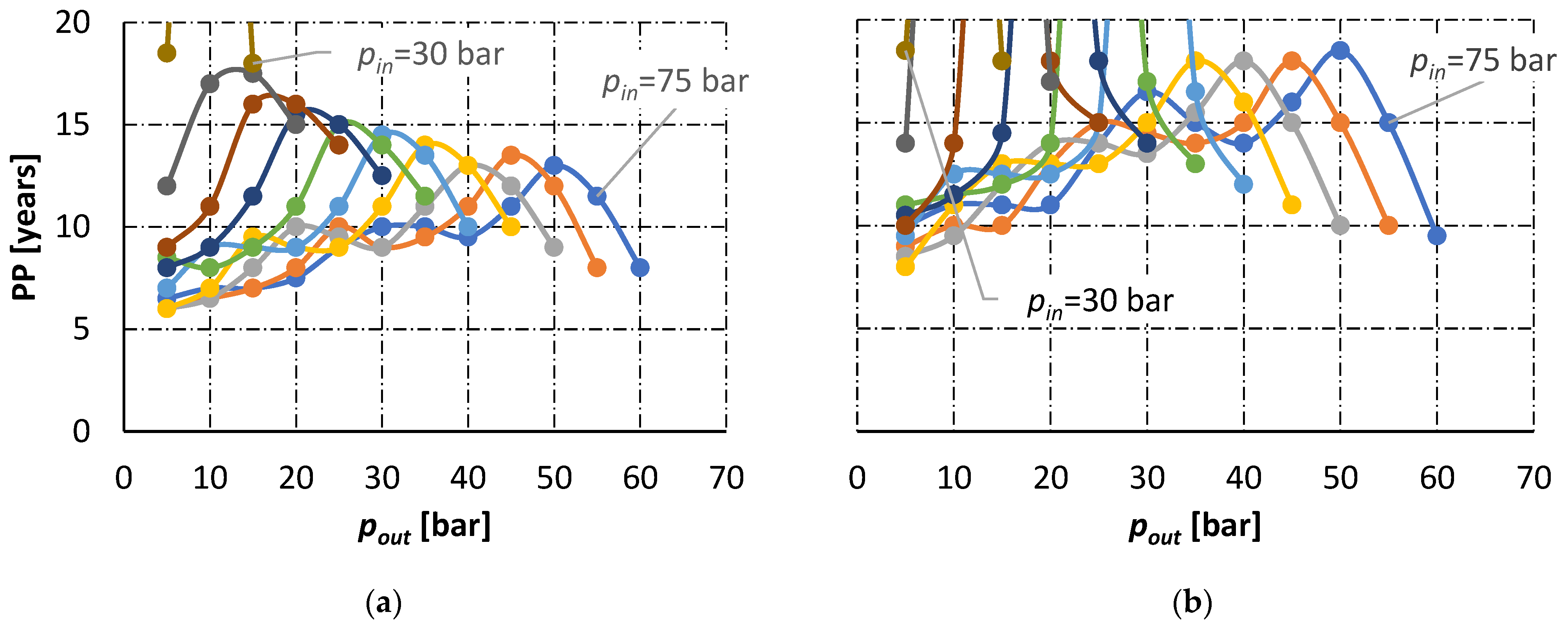
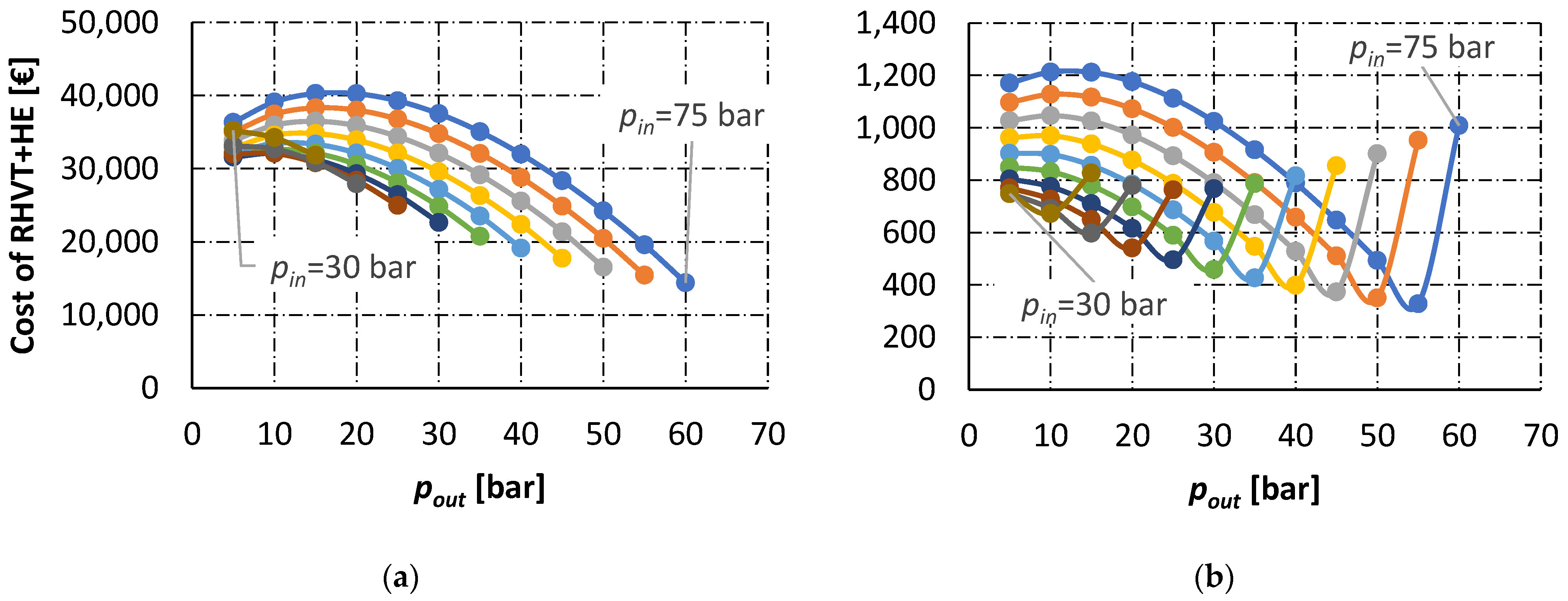
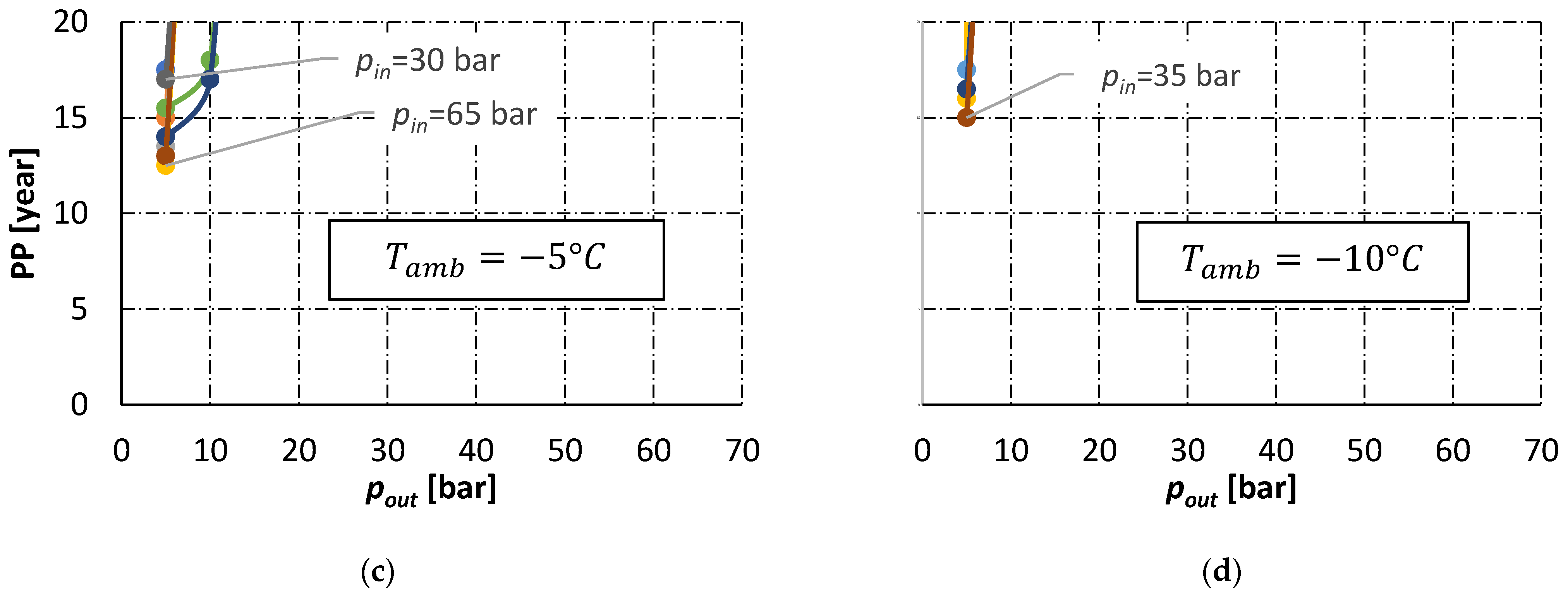
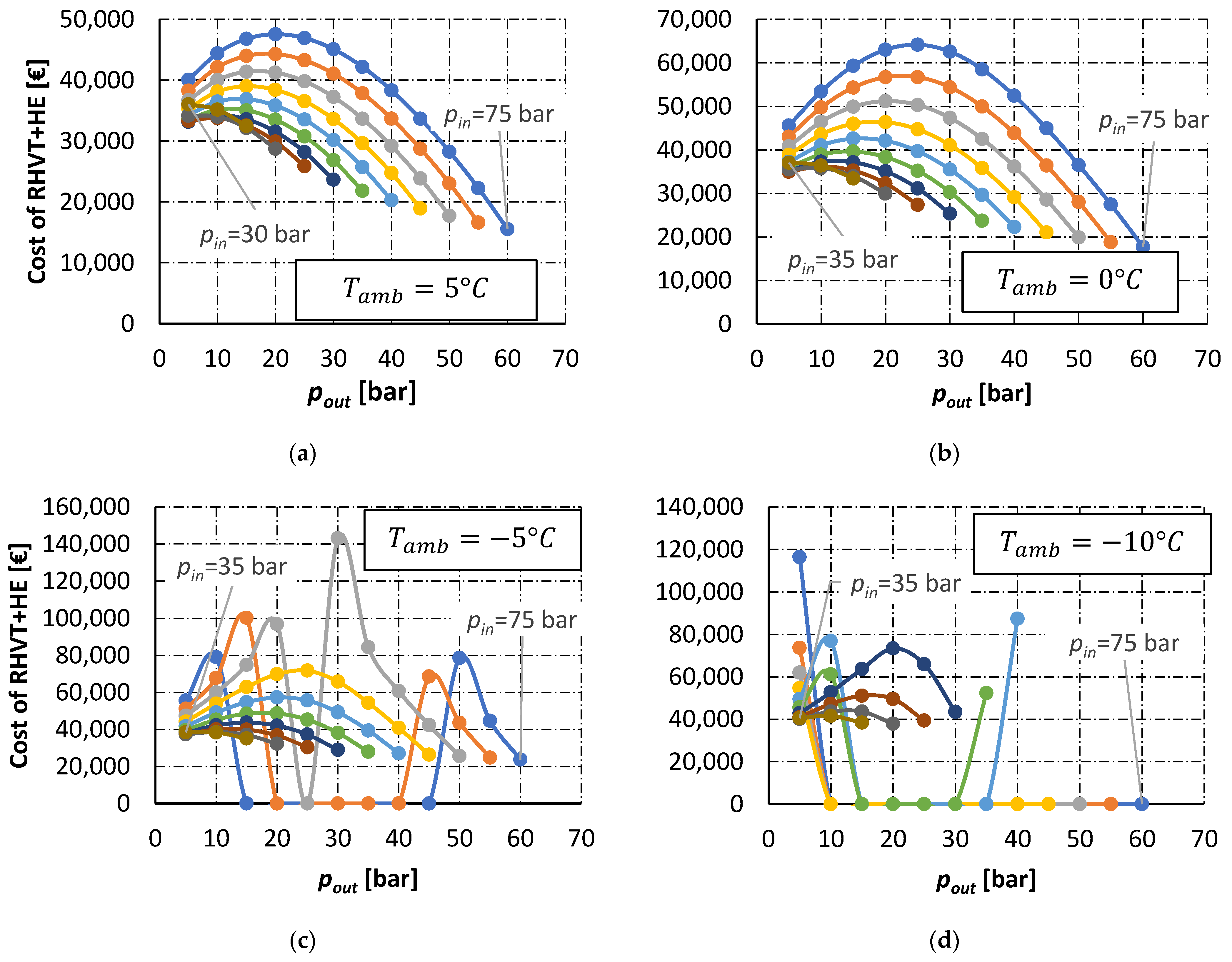
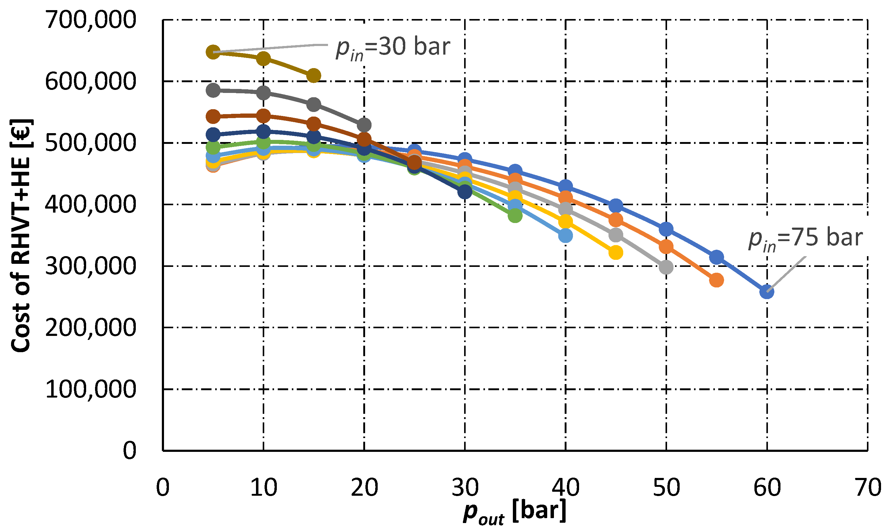
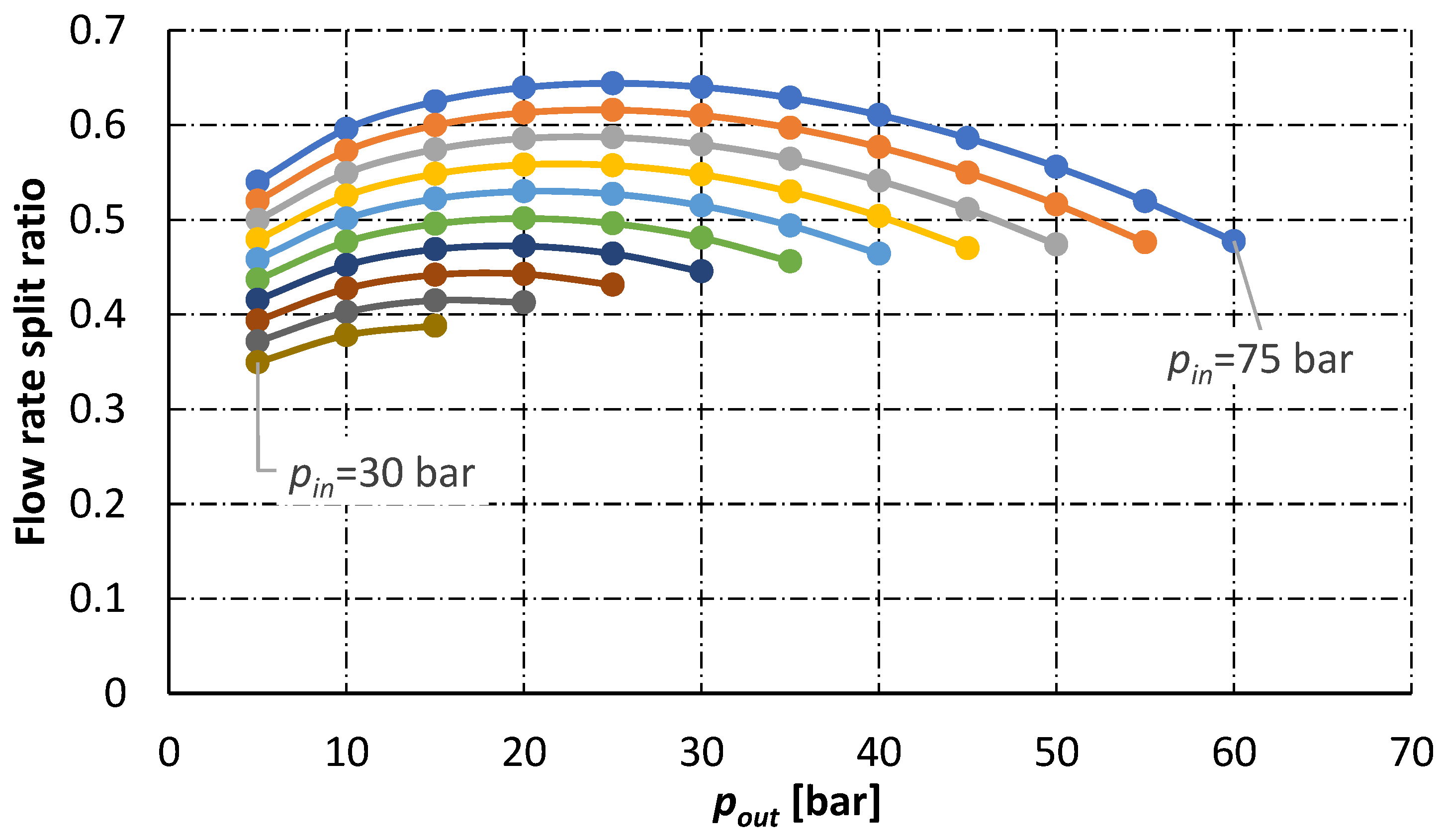
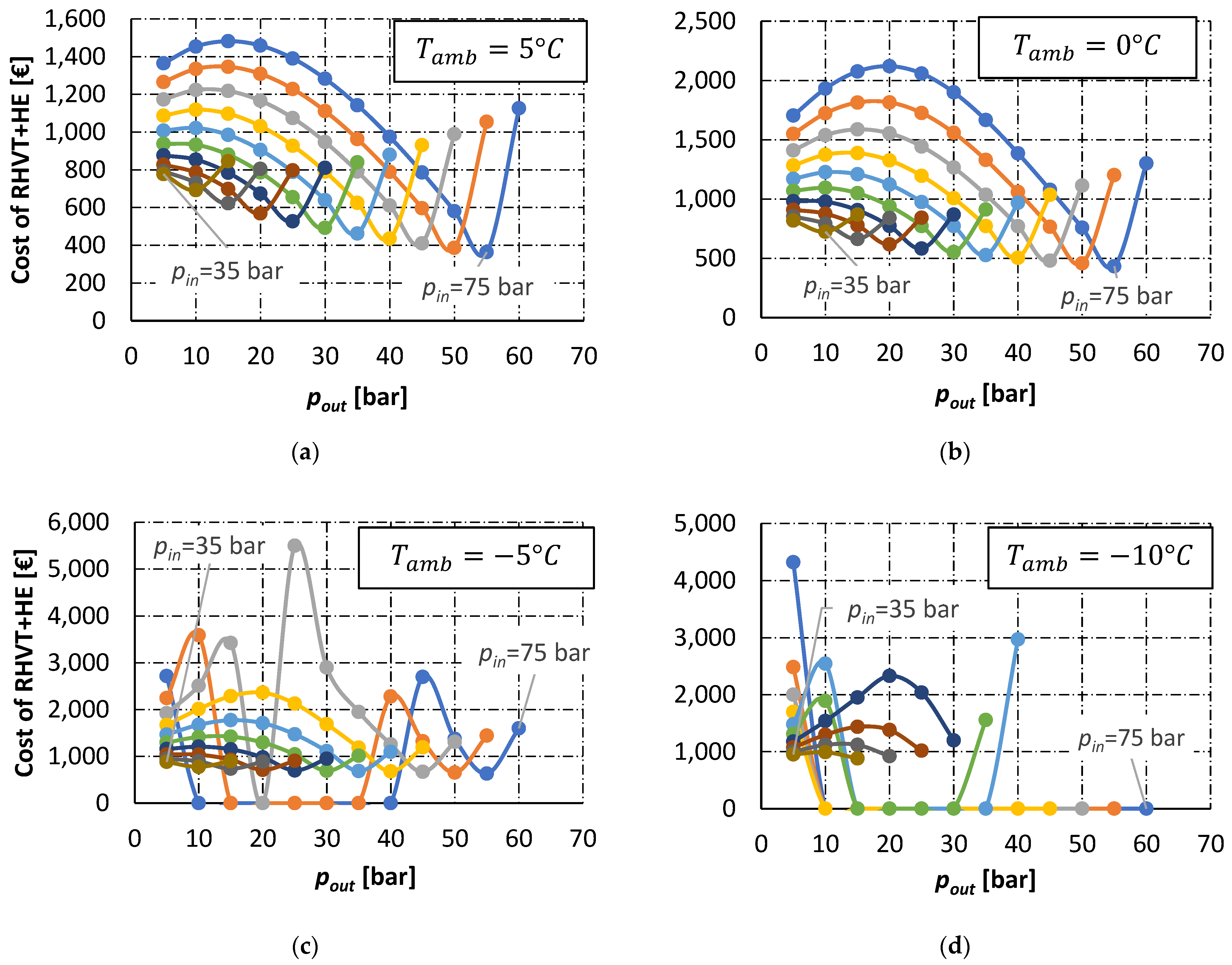
• The PP reaches a maximum at expansion ratios in the range between 2.5 and 3.5. This behaviour is due to the peak in the RHVT flow split, which is responsible for the HE size. As shown in Figure A1, the maximum PP always occurs at expansion ratios between 2.5 and 3.5 and increases as the inlet pressure increases. Analogous confirmation derives from the cost trends shown in Figure A7, Figure A10 and Figure A11;
• A decrease in the size of the PRS tends to increase the overall PP of the system;
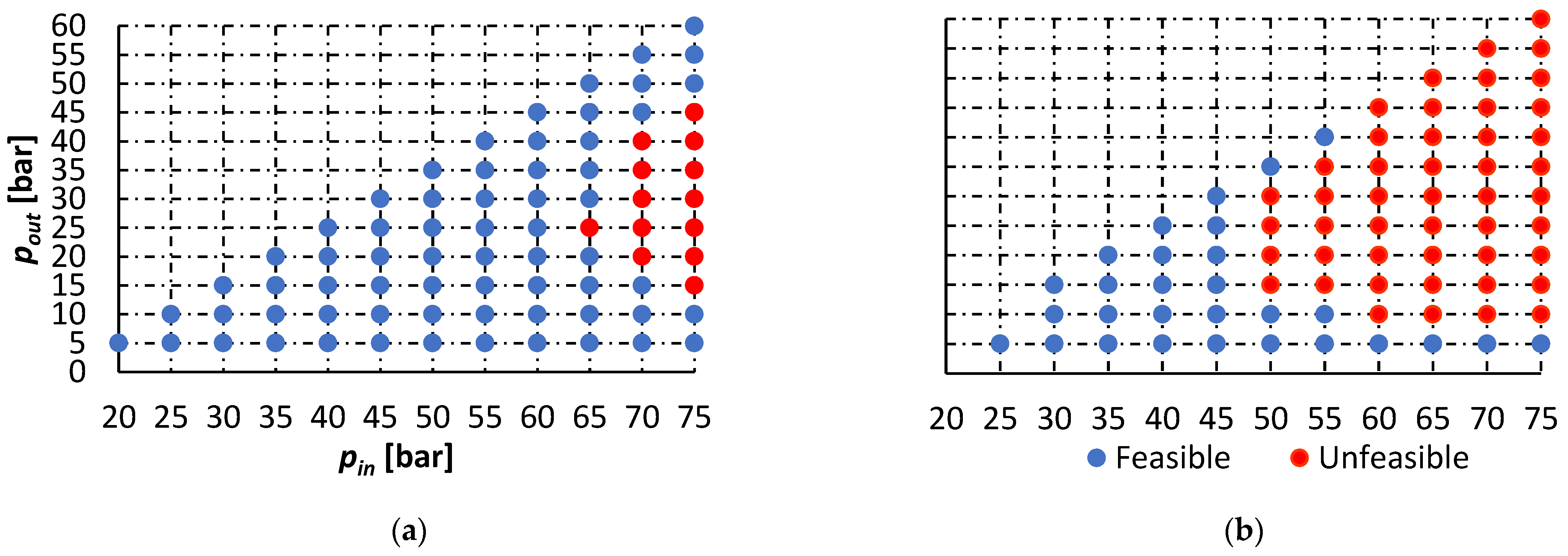
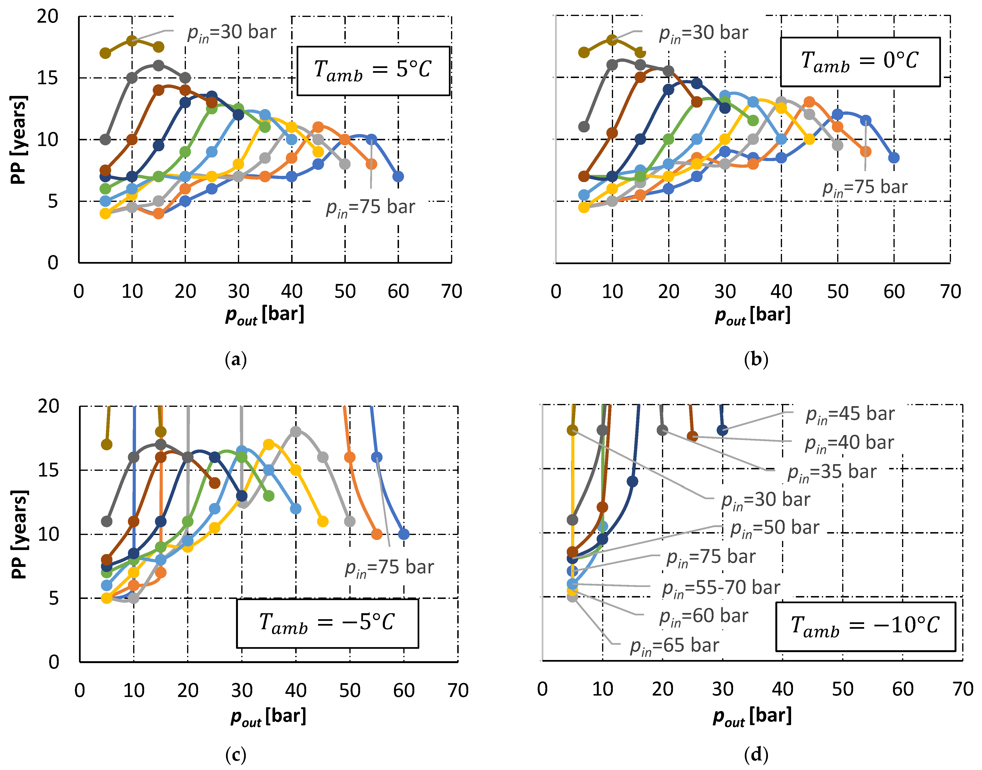
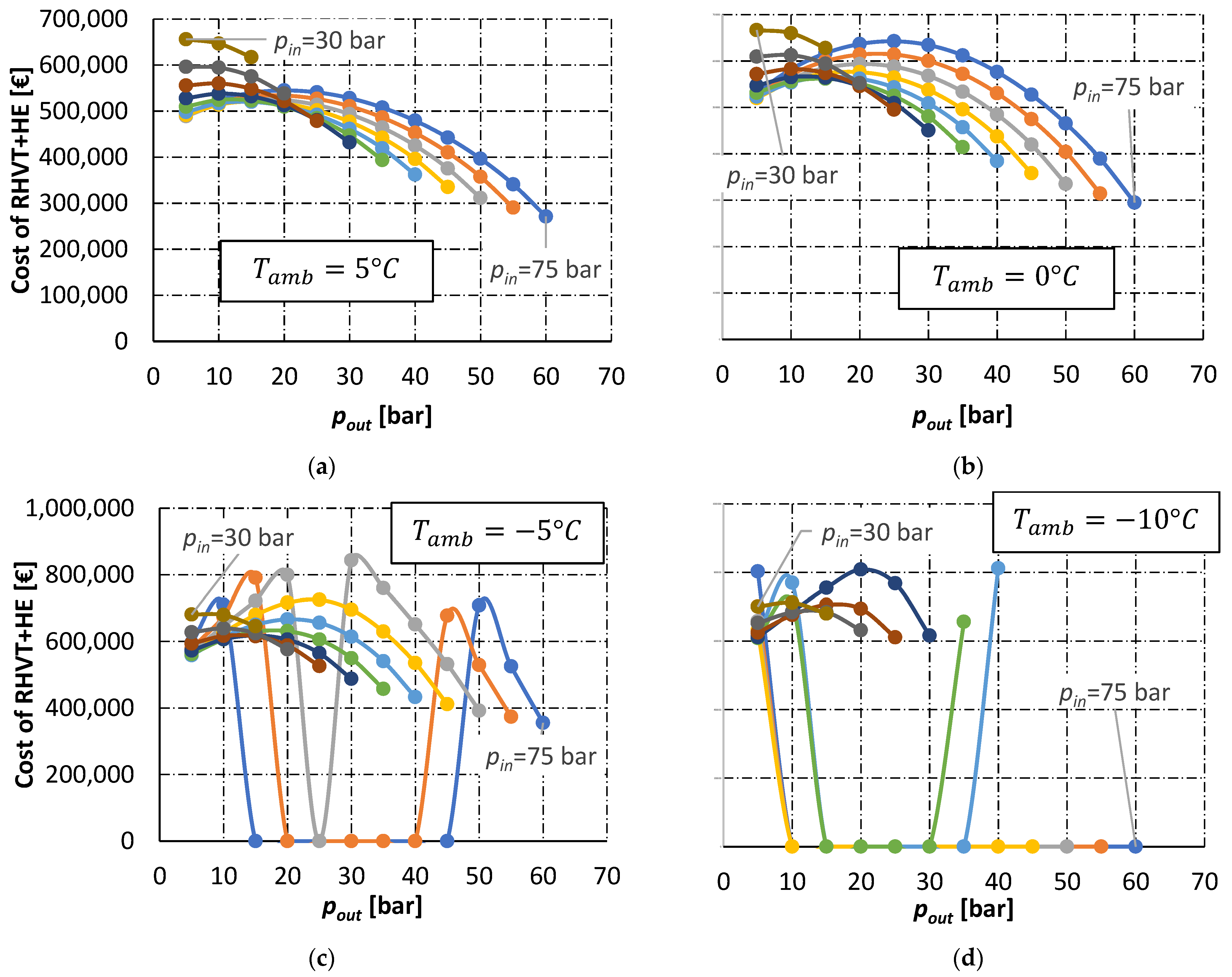
• A decrease in the design ambient temperature leads to an increase in PP, regardless of the PRS size and inlet/outlet pressures. In general, the space of feasible solutions is reduced as the ambient temperature decreases. This statement summarises the results shown in Figure 15, where the technically feasible (blue markers) and unfeasible (red markers) PRS inlet/outlet pressure pairs are reported for ambient temperatures equal to −5 °C in Figure 15a, and −10 °C in Figure 15b. For ambient temperatures above −5 °C, the RHVT–HE system is always technically feasible, regardless of the PRS entrance and exit pressures.

6.2. Potential Application of the RHVT–HE System to the Italian Gas Grid

Figure 16a–e show the PP (the black markers and the secondary y axis), the percentage of PRSs with preheating systems installed in Italy (blue curve), and the corresponding preheating cost savings (red curve) as a function of the averaged volume flow rate processed by the PRS (x axis). In particular, Figure 16a–e refers to the PRS energy recovery systems optimised for 10, 5, 0, −5, and −10 °C ambient temperature operation, respectively. As expected from the general results presented previously, an ambient temperature decrease results in decreased applicability of the proposed RHVT–HE system and the corresponding preheating cost savings. The proposed system does not reach 100% adoption even at a 10 °C ambient temperature. This is because the operating parameters of some PRSs in the Italian grid are not compatible with technically feasible solutions allowed by the considered ambient temperature.

Considering that a design ambient temperature of 0 °C is a reasonable assumption for the entire Italian grid, Figure 16c shows that 96% of the cumulative preheating costs could be avoided by applying the system to 62% of the available stations. Moreover, 80% of NG preheating costs in Italy could be avoided by installing the proposed system in just 6% of the 7412 Italian PRSs if a PP of 16 years or less is acceptable. About 60% of national preheating costs could be avoided by installing the systems into just 2% of PRSs if the maximum PP is 12 years. If a PP shorter than 10 years is required, 40% of preheating costs could still be avoided by installing the system in only 0.6% of PRSs. On the other hand, if an even smaller PP of 8 years or less is expected, only 20% of preheating costs can be saved by installing the system in 0.2% of available PRSs. All of the results just discussed are summarised in

Table 2. Percentage of the total preheating consumptions avoidable (%PH), percentage of the total PRS of the sample using the RHVT–HE system (%PRS), and maximum acceptable PP versus design ambient temperature.

Tamb	10 °C			5 °C			0 °C			−5 °C			−10 °C
	%PH	%PRS	PP	%PH	%PRS	PP	%PH	%PRS	PP	%PH	%PRS	PP	%PH	%PRS	PP
	98.4	91.1	<20	98.3	85.4	<20	96.5	62.1	<20	33.3	23.1	<20	11.6	6.7	<20
	78.7	8.6	<9	78.7	8.6	<11	77.2	7.8	<16	26.6	2.8	<19	9.3	0.6	<16
	59	2.2	<8	59	2.2	<10	57.9	2	<12	20	1	<18	7	0.21	<16
	39.4	0.74	<7	39.4	0.74	<9	38.6	0.7	<10	13.3	0.37	<16	4.6	0.08	<16
	19.7	0.24	<6	19.7	0.24	<7	19.3	0.22	<8	6.7	0.11	<16	2.32	0.04	<16

.

7. Conclusions

This paper investigated the techno-economic feasibility of a novel system to expand NG in the pressure reduction stations of a gas grid. In contrast to the commonly used throttling valves that only reduce the gas pressure, the proposed system is based on coupling an RHVT and an HE to exploit the energy available in the expansion, avoiding NG cooling due to the Joule–Thomson effect. Thus, the economic and environmental costs associated with gas consumption for preheating are saved. First, a techno-economic analysis was conducted to investigate the economic sensitivity of the system to PRS operating parameters. A sample of 240 PRSs was generated to accomplish this, considering an extensive range of operating parameters. A novel empirical model was proposed to predict the performance of the RHVT for the specific application to a PRS, in conjunction with a cost function derived from manufacturers quotations, introduced to evaluate the RHVT cost as a function of its size. The system’s design was optimised for each PRS using a procedure that minimises its overall costs. The results of this analysis led to the following observations:

• It is most convenient to install the system in PRSs working at inlet pressures above 55 bar;
• Expansion ratios lower than 2 penalise the economic feasibility of the system;
• In general, the lower the PRS inlet pressure, the higher the penalty due to low expansion ratios;
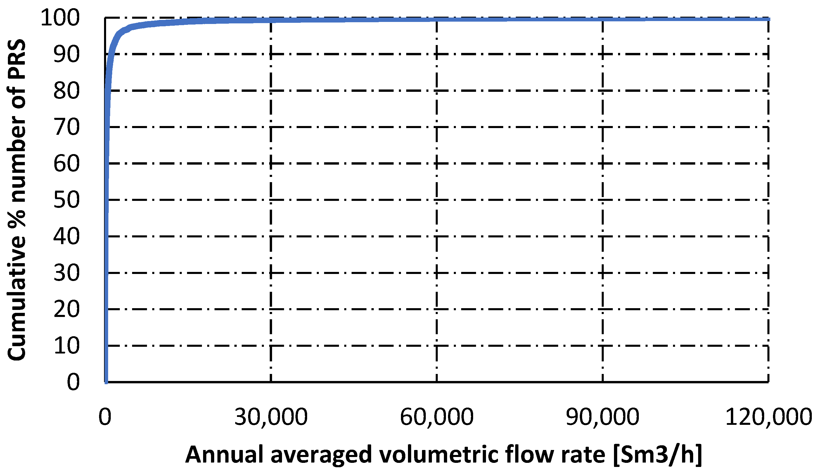
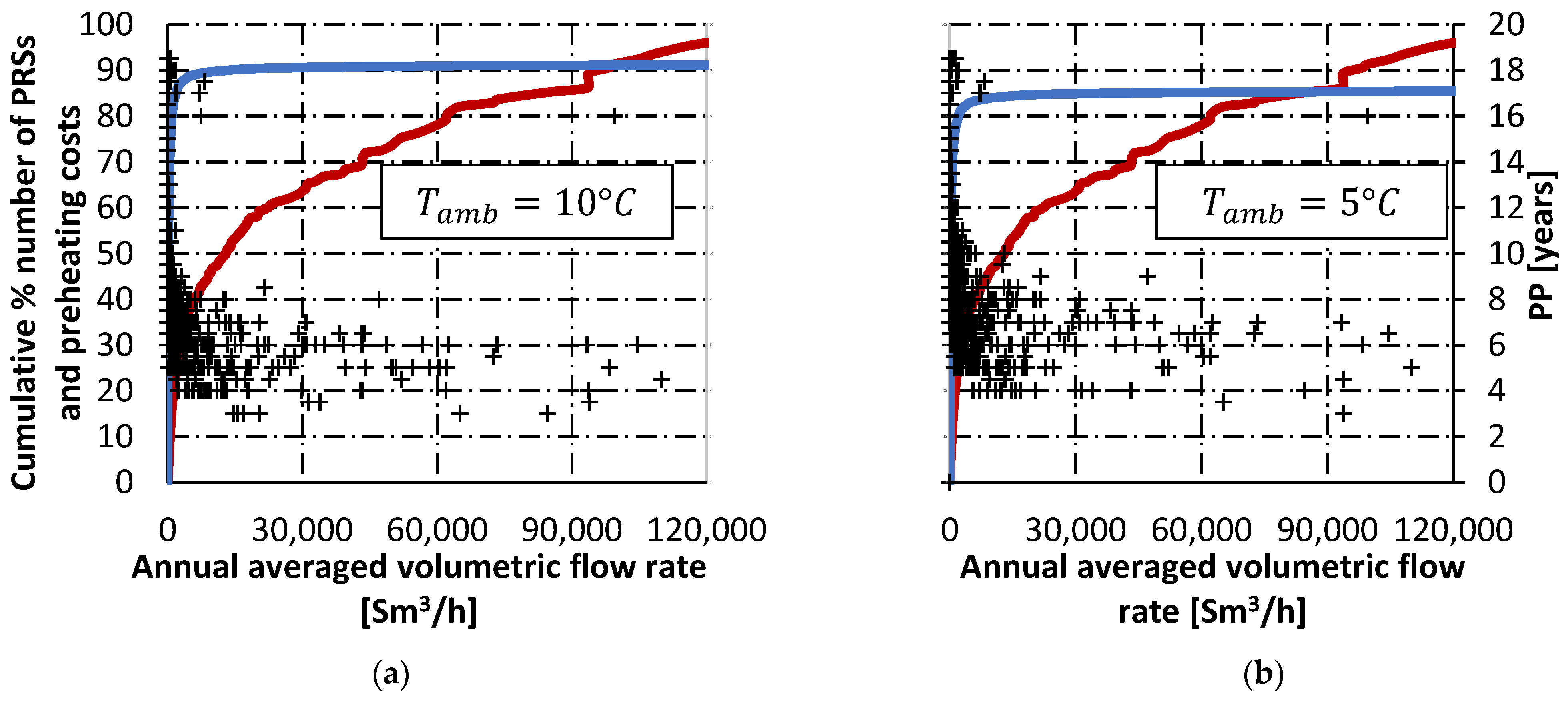
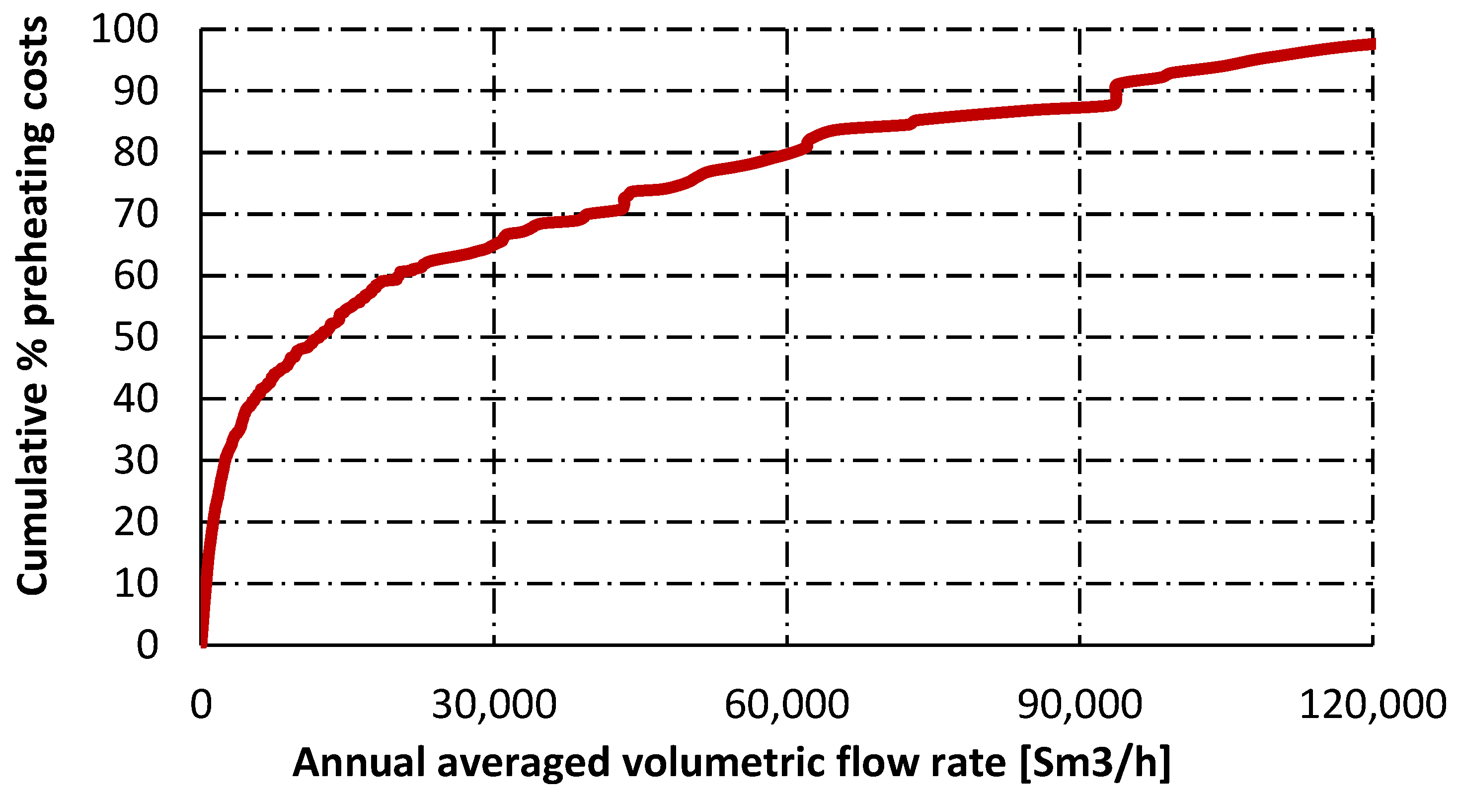
• PRSs having an annual averaged volumetric flow rate below 100 Sm³/h are not economically feasible applications;
• If the design ambient temperature is below 0 °C, the system becomes technically unfeasible for many PRSs.

The design optimisation procedure was also applied to a real case study considering the 7142 PRSs with preheating systems currently installed in Italy. These results led to the following observations:

• It is possible to avoid up to 95% of preheating costs by installing economically feasible systems (PP < 20 years) at a design ambient temperature of 0 °C. If the ambient temperature is reduced to −5 °C and −10 °C, the preheating costs savings are dramatically reduced to 33% and 23%, respectively;
• The system must be installed in locations that impose a design ambient temperature of at least 0 °C to achieve PPs less than 10 years. In particular, an ambient temperature equal to 0 °C allows savings of up to 40% of the preheating costs. The preheating cost savings rise to 80% if the design ambient temperature is at least 5 °C;
• PPs commonly accepted for investment by the industrial sector (on the order of 3.5–4.5 years) can be achieved. For such short PPs, only 25%, 16%, and 3% of the overall preheating costs can be saved at design ambient temperatures of 10 °C, 5 °C, and 0 °C, respectively.

The results of this work definitively demonstrate that the proposed system can drastically reduce NG consumption (and corresponding CO₂ emissions) associated with PRS gas preheating in gas grids. In locations with cold climates, the environmental conditions can limit both the economic and technical feasibility of this system. However, accepting medium-to-long PPs (< 10 years), the system can be successfully installed in many PRSs and locations. Moreover, it should be considered that the price of methane (normally used for preheating) is constantly changing and could rise markedly at any time, making the proposed system much more economically attractive. Energy policies are moving towards requiring higher shares of renewable energy, and additional taxes on fossil fuel consumption could soon be adopted. Although the PPs found in this analysis are not always aligned with the standards of industrial investments, the system’s simplicity is a fundamental advantage for its attractiveness, given that it has no moving parts, no electronics, and does not require any electrical connections.

References

1. Bloch, H.P.; Soares, C. Turboexpanders and Process Applications; Gulf Professional Publishing: Houston, TX, USA, 2001. [Google Scholar]
2. Rheuban, J. Turbo Expanders: Harnessing the Hidden Potential of Our Natural Gas Distribution System. Available online: https://jacobrheuban.com/2009/03/09/turboexpanders-harnessing-the-hidden-potential-of-our-natural-gas-distribution-system/ (accessed on 10 December 2021).
3. Mirandola, A.; Minca, L. Energy Recovery by Expansion of High Pressure Natural Gas. In Proceedings of the 21st Intersociety Energy Conversion Engineering Conference, San Diego, CA, USA, 25–29 August 1986; pp. 16–21. [Google Scholar]
4. Mirandola, A.; Macor, A. Experimental Analysis of an Energy Recovery Plant by Expansion of Natural Gas. In Proceedings of the 23rd Intersociety Energy Conversion Engineering Conference, Denver, CO, USA, 31 July–5 August 1988; pp. 33–38. [Google Scholar]
5. Danieli, P.; Carraro, G.; Lazzaretto, A. Thermodynamic and economic feasibility of energy recovery from pressure reduction stations in natural gas distribution networks. Energies 2020, 13, 4453. [Google Scholar] [CrossRef]
6. Ghezelbash, R.; Farzaneh-Gord, M.; Sadi, M. Performance assessment of vortex tube and vertical ground heat exchanger in reducing fuel consumption of conventional pressure drop stations. Appl. Therm. Eng. 2016, 102, 213–226. [Google Scholar] [CrossRef]
7. Guo, X.; Zhang, B. Experimental investigation on a novel pressure-driven heating system with Ranque–Hilsch vortex tube and ejector for pipeline natural gas pressure regulating process. Appl. Therm. Eng. 2019, 152, 634–642. [Google Scholar] [CrossRef]
8. Hilsch, R. The use of the expansion of gases in a centrifugal field as cooling process. Rev. Sci. Instrum. 1947, 18, 108–113. [Google Scholar] [CrossRef] [PubMed]
9. Lagrandeur, J.; Poncet, S.; Sorin, M. Review of predictive models for the design of counterflow vortex tubes working with perfect gas. Int. J. Therm. Sci. 2019, 142, 188–204. [Google Scholar] [CrossRef]
10. Aswalekar, U.V.; Solanki, R.S.; Kaul, V.S.; Borkar, S.S.; Kambale, S.R. Study and Analysis of Vortex Tube. Int. J. Eng. Sci. Invent. 2014, 3, 51–55, Print: 2319–6726. [Google Scholar]
11. Bilga, P.S.; Kaushik, S.C. Modeling of Temperature Separation Based on Ramming Effect and Heat Exchanger in a Ranque Hilsch Vortex Tube. Int. J. Green Energy 2008, 5, 373–387. [Google Scholar] [CrossRef]
12. Ahlborn, B.; Keller, J.U.; Staudt, R.; Treitz, G.; Rebhan, E. Limits of temperature separation in a vortex tube. J. Phys. D Appl. Phys. 1994, 27, 480–488. [Google Scholar] [CrossRef]
13. Cockerill, T.T. Thermodynamics and Fluid Mechanics of a Ranque Hilsch Vortex Tube. Ph.D. Thesis, University of Cambridge, Cambridge, UK, 1998. [Google Scholar]
14. Xue, Y.; Jafarian, M.; Choudhry, A.; Arjomandi, M. The expansion process in counter-flow vortex tube. Vortex Sci. Technol. 2015, 2, 1000114. [Google Scholar]
15. Bruun, H. Experimental investigation of the energy separation in vortex tubes. J. Mech. Eng. Sci. 1969, 11, 567–582. [Google Scholar] [CrossRef]
16. Biryuk, V.; Gorshkalev, A.; Uglanov, D.; Urlapkin, V.; Korneev, S. A refined model for calculation of the vortex tube thermal characteristics. IOP Conf. Ser. Mater. Sci. Eng. 2018, 302, 12056. [Google Scholar] [CrossRef]
17. Kargaran, M.; Arabkoohsar, A.; Hagighat-Hosini, S.; Farzaneh-Kord, V.; Farzaneh-Gord, M. The second law analysis of natural gas behavior within a vortex tube. Therm. Sci. 2013, 17, 1079–1092. [Google Scholar] [CrossRef]
18. Polihronov, J.G.; Straatman, A.G. The maximum coefficient of performance (COP) of vortex tubes. Can. J. Phys. 2015, 93, 1279–1282. [Google Scholar] [CrossRef]
19. Polihronov, J.G.; Straatman, A.G. The vortex tube effect without walls. Can. J. Phys. 2015, 93, 850–854. [Google Scholar] [CrossRef]
20. Liew, R.; Zeegers, J.C.H.; Kuerten, H.; Michalek, W.R. Maxwell’s demon in the Ranque-Hilsch vortex tube. Phys. Rev. Lett. 2012, 109, 054503. [Google Scholar] [CrossRef] [Green Version]
21. Bej, N.; Sinhamahapatra, K. Numerical analysis on the heat and work transfer due to shear in a hot cascade Ranque–Hilsch vortex tube. Int. J. Refrig. 2016, 68, 161–176. [Google Scholar] [CrossRef]
22. Xue, Y.; Arjomandi, M.; Kelso, R. The working principle of a vortex tube. Int. J. Refrig. 2013, 36, 1730–1740. [Google Scholar] [CrossRef]
23. Xue, Y.; Arjomandi, M.; Kelso, R. Experimental study of the thermal separation in a vortex tube. Exp. Therm. Fluid Sci. 2013, 46, 175–182. [Google Scholar] [CrossRef]
24. Majidi, D.; Alighardashi, H.; Farhadi, F. Best vortex tube cascade for highest thermal separation. Int. J. Refrig. 2018, 85, 282–291. [Google Scholar] [CrossRef]
25. Manimaran, R. Computational analysis of energy separation in a counter-flow vortex tube based on inlet shape and aspect ratio. Energy 2016, 107, 17–28. [Google Scholar] [CrossRef]
26. Aljuwayhel, N.; Nellis, G.; Klein, S. Parametric and internal study of the vortex tube using a CFD model. Int. J. Refrig. 2005, 28, 442–450. [Google Scholar] [CrossRef]
27. Liu, X.; Liu, Z. Investigation of the energy separation effect and flow mechanism inside a vortex tube. Appl. Therm. Eng. 2014, 67, 494–506. [Google Scholar] [CrossRef]
28. Sadeghiseraji, J.; Moradicheghamahi, J.; Sedaghatkish, A. Investigation of a vortex tube using three different RANS-based turbulence models. J. Therm. Anal. Calorim. 2021, 143, 4039–4056. [Google Scholar] [CrossRef]
29. Subudhi, S.; Sen, M. Review of Ranque–Hilsch vortex tube experiments using air. Renew. Sustain. Energy Rev. 2015, 52, 172–178. [Google Scholar] [CrossRef]
30. Sankar Ram, T.; Anish Raj, K. An Experimental Performance Study of Vortex Tube Refrigeration System. Int. J. Eng. Dev. Res. 2013, 17–21. [Google Scholar]
31. Liew, R.; Zeegers, J.C.H.; Kuerten, J.G.M.; Michałek, W.R. Temperature, Pressure and Velocity measurements on the Ranque-Hilsch Vortex Tube. J. Phys. Conf. Ser. 2012, 395, 012066. [Google Scholar] [CrossRef]
32. Williams, A. The cooling of methane with vortex tubes. J. Mech. Eng. Sci. 1971, 13, 369–375. [Google Scholar] [CrossRef]
33. Agrawal, N.; Naik, S.; Gawale, Y. Experimental investigation of vortex tube using natural substances. Int. Commun. Heat Mass Transf. 2014, 52, 51–55. [Google Scholar] [CrossRef]
34. Jafargholinejad, S.; Heydari, N. Simulation of vortex tube using natural gas as working fluid with application in city gas stations. In Proceedings of the 12th International Conference on Heat Transfer, Fluid Mechanics and Thermodynamics, Costa del Sol, Spain, 11–13 July 2016. [Google Scholar]
35. Parker, M.J.; Straatman, A.G. Experimental study on the impact of pressure ratio on temperature drop in a Ranque-Hilsch vortex tube. Appl. Therm. Eng. 2021, 189, 116653. [Google Scholar] [CrossRef]
36. Kirmaci, V.; Kaya, H. Effects of working fluid, nozzle number, nozzle material and connection type on thermal performance of a Ranque–Hilsch vortex tube: A review. Int. J. Refrig. 2018, 91, 254–266. [Google Scholar] [CrossRef]
37. Yilmaz, M.; Kaya, M.; Karagoz, S.; Erdogan, S. A review on design criteria for vortex tubes. Heat Mass Transf. 2009, 45, 613–632. [Google Scholar] [CrossRef]
38. Moraveji, A.; Toghraie, D. Computational fluid dynamics simulation of heat transfer and fluid flow characteristics in a vortex tube by considering the various parameters. Int. J. Heat Mass Transf. 2017, 113, 432–443. [Google Scholar] [CrossRef]
39. Rafiee, S.E.; Sadeghiazad, M.M. Experimental and CFD analysis on thermal performance of Double-Circuit vortex tube (DCVT)-geometrical optimization, energy transfer and flow structural analysis. Appl. Therm. Eng. 2018, 128, 1223–1237. [Google Scholar] [CrossRef]
40. Rafiee, S.E.; Sadeghiazad, M.M. Improving the energetical performance of vortex tubes based on a comparison between parallel, Ranque-Hilsch and Double-Circuit vortex tubes using both experimental and CFD approaches. Appl. Therm. Eng. 2017, 123, 1223–1236. [Google Scholar] [CrossRef]
41. Dincer, K.; Baskaya, S.; Uysal, B.; Ucgul, I. Experimental investigation of the performance of a Ranque–Hilsch vortex tube with regard to a plug located at the hot outlet. Int. J. Refrig. 2009, 32, 87–94. [Google Scholar] [CrossRef]
42. Valipour, M.S.; Niazi, N. Experimental modeling of a curved Ranque–Hilsch vortex tube refrigerator. Int. J. Refrig. 2011, 34, 1109–1116. [Google Scholar] [CrossRef]
43. Im, S.; Yu, S. Effects of geometric parameters on the separated air flow temperature of a vortex tube for design optimization. Energy 2012, 37, 154–160. [Google Scholar] [CrossRef]
44. Mohammadi, S.; Farhadi, F. Experimental analysis of a Ranque–Hilsch vortex tube for optimizing nozzle numbers and diameter. Appl. Therm. Eng. 2013, 61, 500–506. [Google Scholar] [CrossRef]
45. Kumar, G.S.; Padmanabhan, G.; Sarma, B.D. Optimizing the Temperature of Hot outlet Air of Vortex Tube using Taguchi Method. Procedia Eng. 2014, 97, 828–836. [Google Scholar] [CrossRef] [Green Version]
46. Bazgir, A.; Heydari, A.; Bazooyar, B.; Mohammadniakan, M.; Nabhani, N. Numerical investigation of the energy separation effect and flow mechanism inside convergent, straight, and divergent double-sleeve RHVT. Heat Transfer-Asian Res. 2020, 49, 533–564. [Google Scholar] [CrossRef]
47. Cang, R. Optimized Vortex Tube Bundle for Large Flow Rate Applications. Master’s Thesis, Arizona State University, Tempe, AZ, USA, 2013. [Google Scholar]
48. Korkmaz, M.E.; Gumusel, L.; Markal, B. Using artificial neural network for predicting performance of the Ranque–Hilsch vortex tube. Int. J. Refrig. 2012, 35, 1690–1696. [Google Scholar] [CrossRef]
49. Thakare, H.; Monde, A.; Parekh, A.D. Experimental, computational and optimization studies of temperature separation and flow physics of vortex tube: A review. Renew. Sustain. Energy Rev. 2015, 52, 1043–1071. [Google Scholar] [CrossRef]
50. Vortex Tube Technical Datasheet from Vortec, an ITW Company. Available online: https://www.vortec.com/Content/Images/uploaded/literature/Vortex%20Tube%20Brochure%2021’.pdf (accessed on 10 December 2021).
51. Tunkel, L. Eliminating need for gas preheat in pressure regulation. Pipeline Gas J. 2013. [Google Scholar]
Figure 1. (a) Standard isothermal expansion within a PRS with a preheating system; (b) comparison between a gas expansion performed by the Ranque–Hilsch vortex tube (on the right) and a throttling valve (on the left); (c) isothermal expansion performed by the RHVT + HE system.
Energies 15 00371 g001
Figure 2. Heating and cooling effects of the Ranque–Hilsch vortex tube against expansion ratio and mass flow rate split as obtained from experimental data for (a) air and (b) predicted for methane.
Energies 15 00371 g002
Figure 3. (a) Index Z against expansion ratio for x ranging from 0.2 to 0.8; (b) heating and cooling efficiencies against expansion ratio for x ranging from 0.2 to 0.8.
Energies 15 00371 g003
Figure 4. Procedure to calculate the performance of RHVT for pout > pamb.
Energies 15 00371 g004
Figure 5. Comparison between experimental and predicted performance for the expansion of (a) methane and (b) air to pout > pamb.
Energies 15 00371 g005
Figure 6. Cost of RHVT vs. inlet pressure for a constant standard volumetric flow rate (100,000 Sm3/h).
Energies 15 00371 g006
Figure 7. Temperature correction of the hot fluid at the ‘cold side’ of the HE to account for possible ice formation and no forced convection (only natural convection) on the shell side.
Energies 15 00371 g007
Figure 8. Heat exchanger investment cost function.
Energies 15 00371 g008
Figure 9. Dimensionless annual trend of the PRS mass flow rate.
Energies 15 00371 g009
Figure 10. Cumulative percentage distribution of the 7142 PRSs with a preheating system installed in Italy against the annual averaged volume flow rate processed by the entire set of PRSs.
Energies 15 00371 g010
Figure 11. Block scheme of the methodology used to calculate the preheating costs.
Energies 15 00371 g011
Figure 12. Annual preheating cost against outlet pressure for PRSs expanding 100,000 Sm3/h of NG for several inlet pressures values.
Energies 15 00371 g012
Figure 13. Cumulative percentage distribution of preheating costs associated with the operation of 7142 PRSs installed in Italy against the annual averaged volume flow rate of gas processed.
Energies 15 00371 g013
Figure 14. Flowchart of the design optimisation procedure.
Energies 15 00371 g014
Figure 15. Technically feasible (blue) and unfeasible (red) inlet/outlet pressure pairs at ambient temperatures of (a) −5 °C and (b) −10 °C.
Energies 15 00371 g015
Figure 16. PP, percentage of PRSs with preheating systems, and preheating cost savings of the proposed system vs. annual averaged volume flow rate of the PRSs. Ambient temperature equal to (a) 10 °C, (b) 5 °C, (c) 0 °C, (d) −5 °C, and (e) −10 °C.
Energies 15 00371 g016aEnergies 15 00371 g016b