Mixed H₂/H_∞ Optimal Voltage Control Design for Smart Transformer Low-Voltage Inverter

Abstract

The smart transformer has been widely applied for the integration of renewables and loads. For the smart transformer application, the voltage control of low-voltage inverter is important for feeding the load. In this paper, a multi-objective optimization control design approach which comprehensively considers all aspects of indexes, such as linear quadratic (LQ) index, H_∞ norm, and closed-loop poles placement, is proposed based on the linear matrix inequality (LMI) solution. The proposed approach is able to alleviate the weight of the designer from the tedious design process of the multiple resonant controllers and the selection of the weighting matrix for the LQ control. Besides that, some excellent performances such as fast recovering time, low total harmonic distortion (THD) and high robustness are achieved by the proposed approach. The THD are 0.5% and 1.7% for linear and non-linear loads, respectively. The voltage drop for linear load step is reduced to 10 V. The proposed approach is applied to a 5 kVA three-phase inverter to yield an optimal control law. Results from the simulation and experiment presented herein will illustrate and validate the proposed approach.

1. Introduction

The smart transformers (STs) have good application prospects in smart grids and microgrids for the integration of renewables and different AC and DC loads [1,2]. With the increased high proportion of renewable generation, the frequency stability of the power grid brings new challenges due to characteristics strong output uncertainty, poor frequency regulation ability and weak damping for renewables [3,4]. To address the frequency stability, the low-voltage inverter with voltage control (grid-forming inverter) is important for the improvement of the frequency stability when integrating the AC load and low-voltage renewables. Grid-forming inverters are one of the useful inverter applications in microgrid/DERs and are actually voltage-controlled inverters [5,6]. They are functionally similar to uninterrupted power supply (UPS) systems designed to feed the critical loads. In this case, the performance of the inverter is usually assessed in terms of the total harmonic distortion (THD) of the output voltage and the dynamic/steady state responses regardless of load conditions, thereby requiring a load step change in both linear and non-linear loads. To improve the aforementioned performance indexes, plenty of control algorithms have been proposed to apply to inverter control.

The early representative control algorithms were mostly designed by means of the transfer function model based on classical control theory. Those control methods were either multi-loop control [7,8] or single-loop control [9] which are still widely applied today. However, the classical control theory has technical limitations, which include an inability to deal with the multi-input-multi-output system and difficulty in coping with the high order system. Hence, some new methods have been developed. In [10,11], deadbeat control is proposed to achieve fast dynamic response. Nevertheless, most deadbeat approaches are problematic based on their sensitivity to model uncertainties, parameter mismatches, and noise on sensed variables, particularly for high sampling frequencies. In [12], repetitive control is used to accomplish a high-quality sinusoidal output voltage tracking control. Generally, this control technique has a slow response time and is RAM consuming. The sliding mode control has been successful in voltage tracking control for inverters due to major advantages such as strong robustness against parameter variations and external disturbances, fast dynamic response, and simplicity in implementation [13,14], but still, the control technique has a well-known chattering problem. The model predictive control technique for uninterruptible-power-supply (UPS) applications was adopted in [15,16], but the simulation and experimental results fell short in total harmonic distortion (THD). In [17,18], adaptive voltage control is proposed to achieve good performance such as low THD and fast response. However, the calculation of the control law is complex, and load current information is indispensable.

Recently, some interesting control techniques were proposed such as feedback linearization control [19], flatness-based control [20], extended Lyapunov-function-based control [21] and a simple control based on the Kalman filter voltage estimator [22]. The feedback linearization control performs interesting results such as low THD and high dynamic response. The worst disadvantage of this technique is its weakness for parameter uncertainties. The control approaches in [20,21] are very interesting and skillful. The extended Lyapunov-function-based control in [21], for example, designs a specific control law to satisfy the requirement demanding a negative definite derivative for a given dynamical system and eliminates the steady-state error without destroying the global stability of the closed-loop system. Therefore, the control laws are generally complicated; moreover, the load current is necessary for calculating the control law. A simple voltage senseless multi-loop control method has achieved excellent performance according to [22]. Nevertheless, the control method is in essence a variation of state feedback control.

So far, a number of advanced control approaches have been researched in voltage control fields for inverters such as robust control [23,24,25,26] and the linear quadratic regulation (LQR) approach [27,28,29,30,31,32,33,34,35]. Generally, either the robust control or the LQR control are primitively applied to designing the state feedback control to stabilize a system such as the inverted pendulum system. They are usually unable to achieve the zero-steady-error tracking control for the reference (direct current signal or sinusoidal signal). Hence, some extra control approaches, such as incorporating the auxiliary state as the controller [23,24,25,26,27,28,29,30,31,32,33,34] or load current feedforward control [35], must be subjoined to fulfill the function for the inverter control. Basically, according to different reference frames, the selected auxiliary controllers (auxiliary state) are also different. In a rotating reference frame (RRF), the integrator generally is chosen because the sinusoidal signal changes into a direct current (DC) signal in RRF [24,25]. The control law which includes state feedback and tracking terms (the auxiliary state) is designed by means of a linear matrix inequality (LMI)-based optimization where a convergence rate is maximized in [24,25]. While in a stationary reference frame (SRF), the multiple resonant controllers are usually adopted to track the sinusoidal reference signals [26]. However, the high-dimension parameters determination for the multiple resonant controllers is generally not a simple mission [33]. In [26], the design procedure for multiple resonant controllers of a single-phase UPS system is summarized by formulating a convex optimization problem in terms of LMI constraints which is practically the LMI solution of robust optimal H_∞ control. Actually, the different optimization problems with different optimized objectives, which are convergence rates [24,25] and H_∞ norm [23,26] is solved by means of the LMI method to yield the control law. The two optimized indexes sometimes lead to an impracticable control law because of saturation of the control actuator [36]. Besides that, the main shortage of this robust control [23,24,25,26] is that it ignores the physical constraint of the control input so that the design results usually own an overly high bandwidth which can lead to instability. In contrast, the LQR approach preferably considers the problem via minimizing the quantized performance index which includes the control input term. Therefore, the LQR approach has been applied in the voltage control of inverters by many researchers [27,28,29,30,31,32,33,34,35].

Similar to [26], multiple resonant controllers are adopted in [28,29,34]. The difference lies in their employment of the LQR approach to design the control law by means of the function lqr() from MATLAB (MathWorks Inc., Natica, MA, USA) Ufnalski et al. [30,33] utilized the LQR approach to design a control law with an additional integrator plus multiple resonant controller under RRF. However, the primary problem for the LQR method is the selection of the weighting matrix Q for LQR, which is related to the dynamic performance of the system. The selection process is generally a subjective and annoying task, which adopts the trial-and-error method [29,35]. It also requires some high-level expertise and is time-consuming [29,35], especially when the dimensionality of Q is very high, as when multiple resonant controllers are used [26,28,34]. To address this issue, Quan et al. [34] and Ufnalski et al. [33] have adopted the root locus and particle swarm optimization to optimally determine the entries of the weighting matrix Q, respectively. The root locus method in [34] is a pictorial method lacking quantitative analysis. Hence, the result performance may not be optimal. By contrast, an extra user-defined performance index is used to select the best entries of Q in [33], which have achieved a satisfactory result. The performance could be the optimal from an application’s point of view. Nevertheless, user-defined performance index introduced in [33] is calculated by the errors and the differential value of the control input. This is so that the offline determination procedure of the Q depends on the simulation model of the control system because the optimized procedure is continuously implemented through a period of simulation (the simulation time is 6 s in [33]). Otherwise, the procedure should be implemented online, which is impractical for the particle swarm algorithm in real-time control. On the other hand, where the additional state is avoided, the load current feedforward control is used to reduce the steady error in [35]. Therefore, it is virtually a full state feedback control, which is designed by the linear quadratic regulator (LQR) method under the rotating reference frame (RRF). Similarly, the determination of weighting matrix Q is also inevitable.

Generally, the trial-and-error method is needed when designing the high-dimension parameters for the multiple controllers. Moreover, the disturbance-rejection ability and dynamic response are not optimized simultaneously. Therefore, this paper tries to achieve two fundamental purposes: (1) to supply a convenient, systematic and effective design approach for the multiple resonant controllers, and (2) to liberate the designer from the subjective and time-consuming selection of the high-dimension weighting matrix Q for the LQR. Based on these two objectives, this paper converts minimizing of the LQ index into an LMI feasible problem whereby relying on the LMI optimization solver searches out the optimal weight matrix with the additional restraints of H∞ norm and regional poles placement. In this case both disturbance-rejection ability and dynamic response can be optimized. Hence, the two extra restraints are used to regulate the anti-disturbance ability and dynamic and steady performance within the LQR control frame. Finally, a mixed H2/H_∞ optimal voltage control design method is designed. The results in a good compromise between transient performance and disturbance rejection are achieved. The outstanding performance of the proposed approach is verified by simulation and experiment.

2. Modeling for the Control System

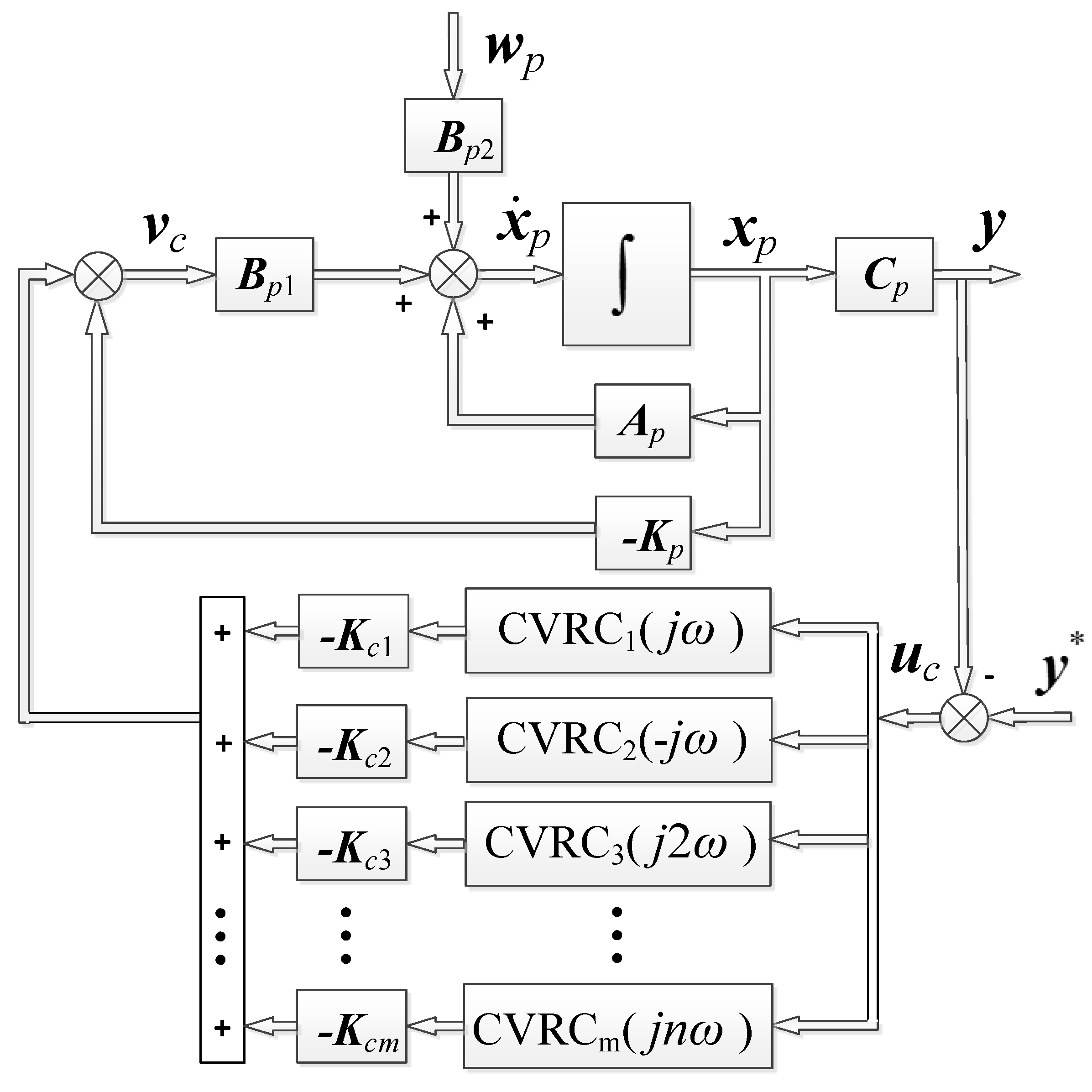
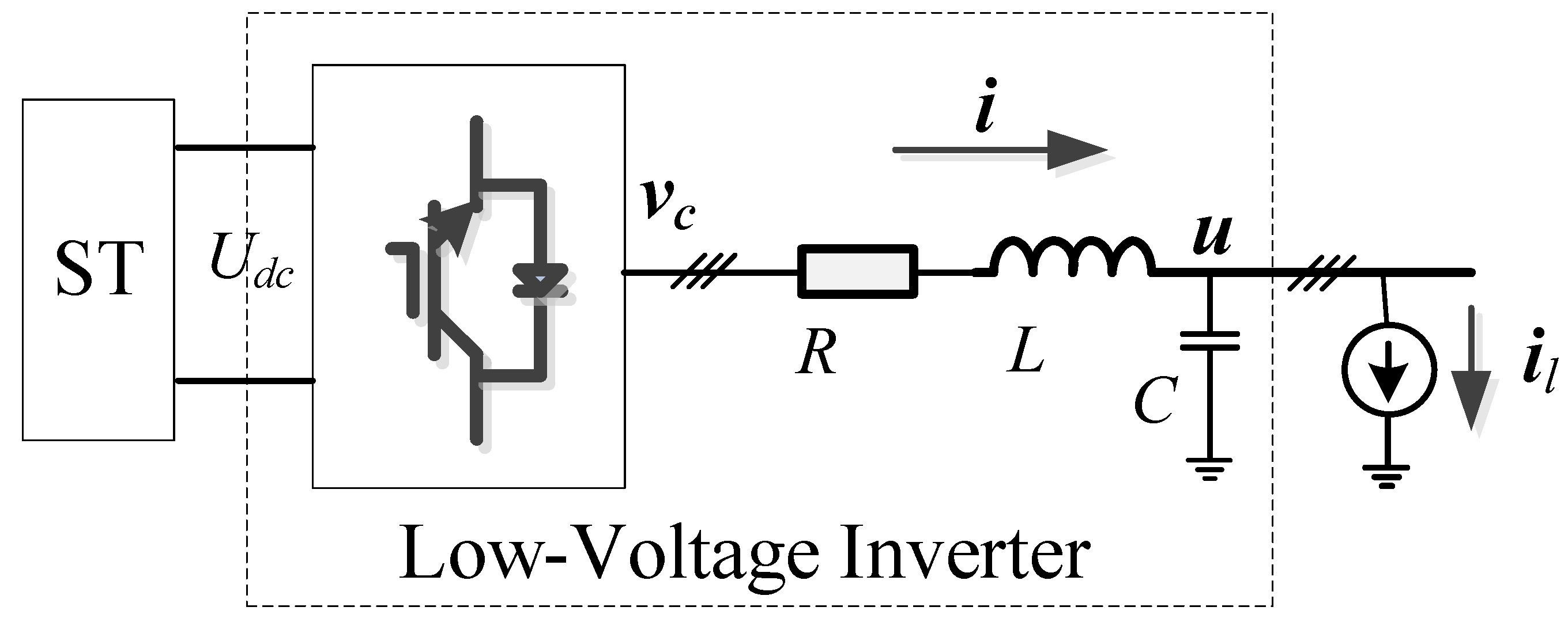
2.1. Modeling for Plant

Figure 1 displays a typical topology of a three-phase inverter with an LC filter. Pulse-width modulation techniques are applied to inverters in order to obtain a sinusoidal output voltage by means of the control input voltage v_c. In this paper, a state space model is adopted to describe the behavior of the inverters [26,34]:

$$\{\begin{array}{c}\begin{array}{c}{\dot{x}}_p=A_p{x}_p+B_{p1}{v}_c+B_{p2}{w}_p\\ \end{array}\\ y=C_p{x}_p\end{array}$$

(1)

To unitedly describe the system for α and β axes, in (1), the state $x_p={\left[i u\right]}^T={\left[i_{\alpha }+j{i}_{\beta }{ }_{ }{u}_{\alpha }+j{u}_{\beta }\right]}^T$ where the boldface variables indicate the complex variables; the inductor current complex variable is shown as i, and the capacitor voltage complex variable is u. $w_p=i_l=i_{l\alpha }+j{i}_{l\beta }$ represents the vector of disturbances from the unknown load current and the voltage of the DC link.

By applying basic electric circuit theory for the LC, the matrices in (1) can be easily derived:

$$A_p=\left[\begin{array}{cc}-\frac{R}{L}& -\frac{1}{L}\\ \frac{1}{C}& 0\end{array}\right]\hspace{1em}{B}_{p1}=\left[\begin{array}{c}\frac{1}{L}\\ 0\end{array}\right]\hspace{1em}{B}_{p2}=\left[\begin{array}{c}0\\ -\frac{1}{C}\end{array}\right]\hspace{1em}{C}_p=\left[\begin{array}{cc}0& 1\end{array}\right]$$

(2)

where the corresponding parameters are shown in the Figure 1. In this model, the assumptions are considered to construct the following optimal voltage controller:

• The disturbances (load currents) is finite energy signals.
• The DC link voltage is well controlled as an ideal DC source by other DC sources such as the battery.

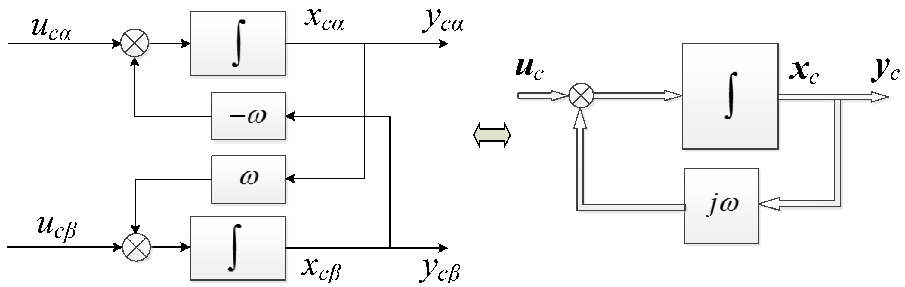
2.2. Complex Variable Resonant Controller

In this section, a brief and intuitive explanation of the complex variable resonant controller (CVRC) is presented. The CVRC transfer function can be expressed as:

$$G_{\mathrm{CVRC}}\left(s\right)=\frac{y_c}{u_c}=\frac{1}{s-j\omega }$$

(3)

from which we can see that the CVRC provides infinite gain only to a positive sequence input complex variable of frequency ω and attenuates the negative sequence complex variable. The CVRC requires fewer states in its implementation, which means less computational load, and provides discrimination between positive and negative sequence signals. This identification of positive and negative sequence signals is an attractive feature, which has been successfully applied to current control for three-phase inverters [37].

In order to design the control parameters for CVRC via modern optimal control theory, we provide the state space expression of the CVRC as:

$$\{\begin{array}{c}{\dot{x}}_c=j\omega x_c+u_c\\ y_c=x_c\end{array}$$

(4)

where $x_c=x_{c\alpha }+j{x}_{c\beta }$, which denotes the auxiliary state variable of the CVRC. The representation of (4) is illustrated in Figure 2 with scale and complex notations, respectively.

2.3. Augmented Modeling for the System

According to the internal model principle, the sinusoidal signal tracking problem may be addressed by means of n resonant controllers, leading to a multiple resonant controller [26,28,29,30,31,32,33,34] in which the multiple scale resonant controllers (MSRCs) are adopted to ensure zero steady-state error for sinusoidal tracking control and, equivalently, reject the asymptotic disturbance of sinusoidal signals. Analogously, the multiple CVRCs (MCVRCs) are employed to achieve the same function with the closed-loop structure depicted in Figure 3 where n = ±1, ±2… denotes the order of the CVRCs, and m represents the number of the CVRCs. It is worth noting that the MCVRCs are not an exclusive option for the application in this paper, but they are employed mainly because of their attractive feature, which supplies simple control implementation for αβ axes. MSRCs could equally be chosen to accomplish the control task in three-phase inverter applications for the proposed design approach.

As is depicted in Figure 3, the CVRCs and the model of the plant are connected by means of setting the input of the CRVCs to equal the error of the output voltage:

$$u_c=y^{*}-C_p{x}_p$$

(5)

Substituting (5) into (4), then combining (1), we can derive the augmented state space model of the control system as:

$$\{\begin{array}{c}\dot{x}=Ax+B_1{v}_c+B_2{w}_p+R{y}^{*}\\ y=Cx\end{array}$$

(6)

where $x={[x_p x_{c1} x_{c2}\cdots x_{cm}]}^T$ represents the augmented state variables and $y^{*}$ denotes output voltage complex variable reference. The corresponding state describing matrices are:

$$A=\left[\begin{array}{cccccc}{A}_p& & & & & \\ -C_p& j\omega & & & & \\ -C_p& & -j\omega & & & \\ ⋮& & & \ddots & & \\ -C_p& & & & jn\omega & \\ -C_p& & & & & -jn\omega \end{array}\right]$$

(7)

$$B_1={\left[\begin{array}{cccccc}{B}_{p1}& 0& 0& \cdots & 0& 0\end{array}\right]}^T$$

(8)

$$C=\left[\begin{array}{cccccc}{C}_p& 0& 0& \cdots & 0& 0\end{array}\right]$$

(9)

$$B_2={\left[\begin{array}{cccccc}{B}_{p2}& 0& 0& \cdots & 0& 0\end{array}\right]}^T$$

(10)

$$R={\left[\begin{array}{cccccc}0& 1& 1& \cdots & 1& 1\end{array}\right]}^T$$

(11)

From (7) to (11), we find that it is very convenient to revise those matrices if the number of CVRCs is changed. The dimensions of those matrices are related to the number of the CVRCs: d = m + 2. The variable d denotes the dimension as well the number of complex state variables. In addition, for m CVRCs, there are m + 2 undetermined complex parameters which means that 2 m + 4 real parameters need to be tuned, as shown in Figure 3, and are included by the augmented state feedback control law such that:

$$v_c=-Kx=-\left[K_{p1}^{\left(i\right)} K_{p2}^{\left(u\right)} K_{c1}^{\left(+1\right)} K_{c2}^{\left(-1\right)} K_{c3}^{\left(+2\right)} K_{c4}^{\left(-2\right)} \cdots K_{cm}^{\left(+n\right)}\right]x$$

(12)

Depending on the number of CVRCs to be used, it should be emphasized that the design of those parameters is not a facile task for a large number of CVRCs when the objective is to accomplish the control performance of a small tracking error, attenuation of harmonic distortion, and fast recovering time for sudden load variations. Furthermore, classical control theory methods such as root locus design are difficult to handle or even impractical for such a large number of parameters. Therefore, Section 3 will illustrate in detail a systematic and analytical approach to determine multiple controllers’ parameters.

3. Control Parameter Design

As previously stated: all complex control parameters can be determined by means of designing the state feedback control law K of the augmented system (6). Generally, the state feedback control law in this paper’s condition can be tuned in at least three different ways: The linear quadratic regulation (LQR) solution which is solved by the algebraic Riccati equation, or direct tuning of the controller gain matrix K, or using the closed-loop system pole placement method [33]. Among these three approaches, the LQR design method is considered the best choice for achieving good performance. LQR design also has some other advantages, which include inherently stable and relatively simple in solving the optimization problem analytically, e.g., lqr() or dlqr() in MATLAB or Scilab environments. For the LQR method, the selection of weighting matrixes Q and R is both a crucial and tedious step which generally is fulfilled by guessing and checking, and at the same time, involving expert knowledge and the opinions of its researchers.

Hence, in this research, the linear quadratic (LQ) index was handled by means of the linear matrix inequality (LMI) approach, which can be solved in MATLAB. However, the LMI toolbox in MATLAB can only deal with the real number LMI; therefore, we must first convert the complex number LMI into a real one. Considering the following map relationship between a complex variable and matrix:

$$a+jb\triangleq \left[\begin{array}{cc}a& -b\\ b& a\end{array}\right]$$

(13)

which constructs the isomorphic relations between the complex space and real matrix space $R^{2\times 2}$, complex matrix can be equivalently expressed by a dimension-added real matrix, after which, the corresponding complex variables become dimension-added real vectors:

$$\left(a+jb\right)\left(u_{\alpha }+j{u}_{\beta }\right)\iff \left[\begin{array}{cc}a& -b\\ b& a\end{array}\right]\left[\begin{array}{c}{u}_{\alpha }\\ u_{\beta }\end{array}\right]$$

(14)

We suppose hereafter that (6) represents the equivalent dimension-added real matrixes and the dimension-added real vectors without influencing the correctness of the statement. Therefore, the discussion of the next LMI-based parameters design is in terms of real number.

3.1. Linear Quadratic (LQ) Control

Defining the LQ cost:

$$J={{\displaystyle \int }}_0^{\infty }\left(x^T\left(t\right)Qx\left(t\right)+u^T\left(t\right)Ru\left(t\right)\right)dt$$

(15)

where superscript “T” represents transposition and Q ≥ 0, R > 0, for the real notation of the system (6), we have the following theorem.

Theorem 1.

If there exists a symmetric positive definite matrix P satisfying the matrix inequality:

$$Q+K^{T}RK+P\left(A-B_{1}K\right)+{(A_{}-B_{1}K)}^{T}P<0$$

(16)

then, the$v_c=-Kx$is a guaranteed cost control law for real notation of the system (6) which ensures:

• The closed-loop steady and
• The LQ index$J\le J^{*}=x_0^{T}P{x}_0$.

Proof of Theorem 1.

Primarily, writing the closed-loop system with the function of the control law $v_c=-Kx$:

$$\dot{x}=\left(A-B_{1}K\right)x+B_2{w}_p+R{y}^{*}$$

(17)

then, by defining the Lyapunov function $V\left(x\right)=x^{T}Px$, we can derive the derivative of the Lyapunov function:

$$\dot{V}\left(x\right)=x^T\left[P\left(A-B_{1}K\right)+{\left(A-B_{1}K\right)}^{T}P\right]x$$

(18)

with the status of zero input. Applying (16), the inequality

$$\dot{V}\left(x\right)=x^T\left[P\left(A-B_{1}K\right)+{\left(A-B_{1}K\right)}^{T}P\right]x\le -x^T\left[Q+K^{T}RK\right]x<0$$

(19)

is tenable for the model. According to the Lyapunov stability theory, the model is asymptotically stable. The property (1) is proved. For property (2), integrating from zero to infinity for both sides of (19), we have:

$${{\displaystyle \int }}_0^{\infty }{x}^{T}Qx+u^{T}Rudx\le -{{\displaystyle \int }}_0^{\infty }\dot{V}\left(x\right)dx=x_0^{T}P{x}_0$$

(20)

The equality in (20) is deduced from the robust stability with $V(\infty )=0$. Up to this point the Theorem 1 has been proved. □

Paying attention to the minimum cost $J^{*}=x_0^{T}P{x}_0$, which depends on the initial state x₀, in practice, we suppose that the initial state x₀ is a zero-expectation random variable satisfying $E\left(x_0{x}_0^T\right)=I$ where I denotes the identity matrix. Hence, we can deal the index with $J^{*}=E\left(x_0^{T}P{x}_0\right)=Trace\left(P\right)$ where Trace() means to seek matrix trace. Simultaneously, in awareness of the non-linearity of the inequality (16), we provide Theorem 2, which gives a feasible solution for the inequality by means of LMI.

Theorem 2.

For the model (16) and given R, if there exists a symmetric positive definite matrix W₁, positive matrixes M and Q_inv and matrix V₁ making the convex optimization problem:

$$\underset{W_1, V_1, M, Q_{inv}}{min} Trace(M)$$

(21)

$$\left[\begin{array}{ccc}\left(A{W}_1-B_1{V}_1\right)+{(A{W}_1-B_1{V}_1)}^T& W_1& V_1{}^T\\ W_1& -Q_{inv}& \\ V_1& & -R^{-1}\end{array}\right]<0$$

(22)

$$\left[\begin{array}{cc}M& I\\ I& W_1\end{array}\right]>0$$

(23)

feasible with the solution${\widehat{W}}_1,{\widehat{V}}_1,\widehat{M},{\widehat{Q}}_{inv}$, then the$v_c=-Kx=-{\widehat{V}}_1{\widehat{W}}_1^{-1}x$is the robust guaranteed index control law with the minimum index upper bound:

$$\widehat{J}={{\displaystyle \int }}_0^{\infty }\left(x^T{\widehat{Q}}_{inv}^{-1}x+u^{T}Ru\right)dt=Trace(\widehat{M})$$

(24)

Proof of Theorem 2.

From (16), by applying the Schur complement [38], we can deduce the LMI

$$\left[\begin{array}{ccc}P\left(A-B_{1}K\right)+{(A-B_{1}K)}^{T}P& I& K^T\\ I& -Q^{-1}& \\ K& & -R^{-1}\end{array}\right]<0$$

(25)

which is equivalent with (16). Pre- and post-multiplying the above LMI by diag([P⁻¹, I, I]), where diag() denotes the diagonal matrix, and defining $W_1=P^{-1}$, $V_1=K{P}^{-1}=K{W}_1$ yields the following constraints:

$$\left[\begin{array}{ccc}\left(A{W}_1-B_1{V}_1\right)+{(A{W}_1-B_1{V}_1)}^T& W_1& V_1{}^T\\ W_1& -Q^{-1}& \\ V_1& & -R^{-1}\end{array}\right]<0$$

(26)

Then according to Theorem 1, the $v_c=-Kx=-V_1{W}_1^{-1}x$ is a robust guaranteed index control law with the performance index:

$$J^{\ast }=Trace\left(P\right)=Trace\left(W_1^{-1}\right)$$

(27)

To avoid selecting the weighting matrix Q, we change the user-defined Q to an optimization variable $Q^{-1}=Q_{inv}$ to extend the feasible region. This is an important procedure, referred to as QP, which has benefits through the removal of the subjective Q selection task and enlarges the feasible region. After this procedure, (22) is acquired. However the R is reserved in (22) because we need to take adequate control input into account to avert overlarge amounts of the control input.

Within the feasible region $\left(W_1,V_1,M,Q_{inv}\right)$, we search the upper bound of the index $Trace\left(W_1^{-1}\right)$ which is not a linear optimization problem; therefore, (23) is introduced to resolve this problem. Based on the Schur complement, (23) is equivalent to $M>W_1^{-1}>0$ which implies that the minimizing $Trace(M)$ ensures the minimization of $Trace\left(W_1^{-1}\right)$. Therefore, Theorem 2 has been proved. □

The LMI-style constraint (22) for LQ index owns a very high degree of freedom when the QP is done to endow the optimization solver with the decision power of Q. Furthermore, the LQ index does not consider the dynamic response of the control system. Therefore, in general, the control law yielded from the optimization problem (21) is super small; hence its results are too small to achieve satisfactory dynamic performance. Consequently, we increase the extra H∞ norm constraint, which supplies the robust ability of rejecting external disturbance, and poles region constraint, which tunes the dynamic behaviors of the control system.

3.2. H_∞ Norm Constraint

Applying the well-known bounded real lemma [38,39], to the closed-loop system (17), the following Theorem 3, which was certified in [26], is given in the sequence.

Theorem 3.

For the closed-loop system (17), if there exists a positive real number $\gamma$, a symmetric positive definite matrix W₂ and matrix V₂ getting the convex optimization problem:

$$\underset{\gamma , W_2, V_2}{min} \gamma$$

(28)

$$\mathrm{s}.\mathrm{t}. \left[\begin{array}{ccc}\left(A{W}_2-B_1{V}_2\right)+{(A{W}_2-B_1{V}_2)}^T& B_2& W_2{C}^T\\ B_2^T& -\gamma I& \\ C{W}_2& & -\gamma I\end{array}\right]<0$$

(29)

feasible with the solution$\widehat{\gamma }, {\widehat{W}}_2, {\widehat{V}}_2$, then$v_c=-Kx=-{\widehat{V}}_2{\widehat{W}}_2^{-1}x$is the robust optimal H∞ state feedback control law with the minimum H∞ norm:

$$\Vert T_{w_{p}y}{\left(s\right)\Vert }_{\infty }=\underset{\Vert w_p\Vert \ne 0}{sup}\frac{{\Vert y\Vert }_2}{\Vert w_p\Vert {}_2}\le \widehat{\gamma }$$

(30)

The closed-loop system is stable.

The detailed proof of Theorem 3 could be referred in [26,38,39]. Theorem 3 maximizes the capacity of resisting the perturbance by means of minimizing the H∞ index otherwise ignoring the practical physical limitation of the control input. Hence, the control law from the optimization problem (28) often leads to an impractical control scheme which will be proved by the experiment. In this paper, the LMI (29) is adopted solely as a constraint to consistently tune the perturbance-rejection performance.

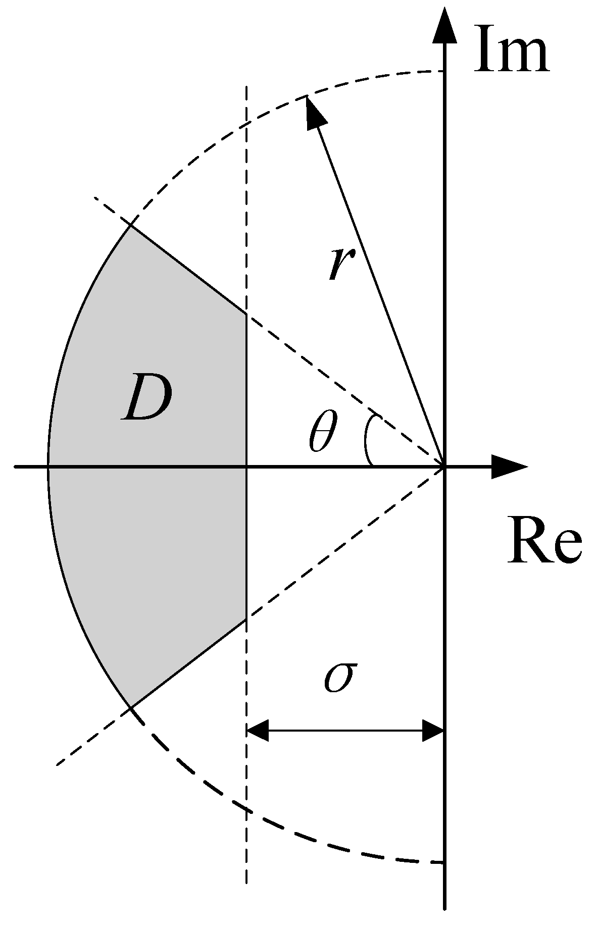
3.3. Poles Region Constraint

It is well known that the transient response of a linear system is related to the location of the poles. Therefore, the regional poles placement (RPP) method was adopted to ensure the transient performance for system dynamics, such as exponential convergence rate, natural frequency, and damping factor [26,40]. The LMI region $D\left(\sigma ,r,\theta \right)$, as shown in Figure 4, confines the closed-loop poles to this region with a minimum exponential attenuation rate σ, a minimum damping ratio ξ = cos(θ), and the natural frequency r. This in turn bounds the maximum overshoot, the frequency of oscillatory modes, the settling time and the attenuation time [40]. Because the approach permits the optimization solver searching the Q itself, the RPP is used to regulate the dynamic behavior of the system in an auxiliary way.

The RPP with the LMI region $D\left(\sigma ,r,\theta \right)$ is formulated in terms of the concept of D-stability which is described by the following LMI constraints [26,40]:

$$L_j\otimes W_3+M_j\otimes \left(A{W}_3-B_1{V}_3\right)+M_j^T\otimes {\left(A{W}_3-B_1{V}_3\right)}^T<0, \begin{array}{c}j=1,2,3\end{array}$$

(31)

where $\otimes$ denotes the Kronecker product of matrices, and W₃ is a symmetric positive definite matrix; the corresponding matrices L_j and M_j are referred in [26,40].

As long as the LMI constraints (31) are satisfied for the symmetric positive definite matrix W₃ and V₃ = KW₃, then System A is the robust D-stability which implies that all of poles of the closed-loop system A are placed in region $D\left(\sigma ,r,\theta \right)$.

3.4. The Comprehensive Optimization

Observing the LMI constraints (22), (23), (29) and (31), it is obvious that the LMI constraints are not convex for the optimized variables W₁, W₂, W₃, V₁, V₂ and V₃ so that the feasibility of the LMI constraints is generally difficult to resolve. To overcome this difficulty, after defining the common optimized variable as:

$$W=W_1=W_2=W_3, V=KW$$

(32)

we can then derive the following multi-objective convex optimization problem with LMI constraints:

$$\underset{\gamma , W, V,\begin{array}{c}\end{array}M, Q_{inv}}{min} a\gamma +bTrace(M)$$

(33)

s.t. (22), (23), (29) and (31), which can be resolved by the solver mincx() in the LMI toolbox of MATLAB. If the convex optimization problem (33) is feasible with the solution $\widehat{\gamma }, \widehat{W}, \widehat{V}, \widehat{M}, {\widehat{Q}}_{inv}$, the $v_c=-Kx=-\widehat{V}{\widehat{W}}_{}^{-1}x$ is the robust optimal state feedback control law with the minimum performance index $a\widehat{\gamma }+bTrace(\widehat{M})$.

The upper convex optimization problem asks for a common optimized matrix W which introduces some conservative properties, but it greatly facilitates the solving of the optimization problem.

The coefficients a and b in (33) are weights used to compromise between the H_∞ norm and LQ index. However, in this paper, a and b are only selected from logic number 0 or 1 to avoid the troublesome and subjective weight selection. The different coefficients combinations are illustrated in

Table 1. Illustration of the different combinations of the coefficients.

Scheme	a	b	Significance
①	0	0	no optimization
②	0	1	optimal LQ index with regional closed-loop pole placement
③	1	0	optimal H∞ norm with regional closed-loop pole placement
④	1	1	optimal H∞ norm plus LQ index with regional closed-loop pole placement

. Actually, when the predictable linear load uncertainty is considered as the polytypic model, the combination ③ would become the approach proposed in [26].

As a result, the design procedure of the proposed optimal control law can be summarized as follows.

Step (1)

Build augmented system model (6).

Step (2)

Establish the LMI constraint (22) and (23) with the identity matrix R.

Step (3)

Establish the LMI constraint (29).

Step (4)

Establish the LMI constraint (31) with the selectable region $D\left(\sigma ,r,\theta \right)$

Step (5)

Based on the selected a and b, solve the optimization problem (33).

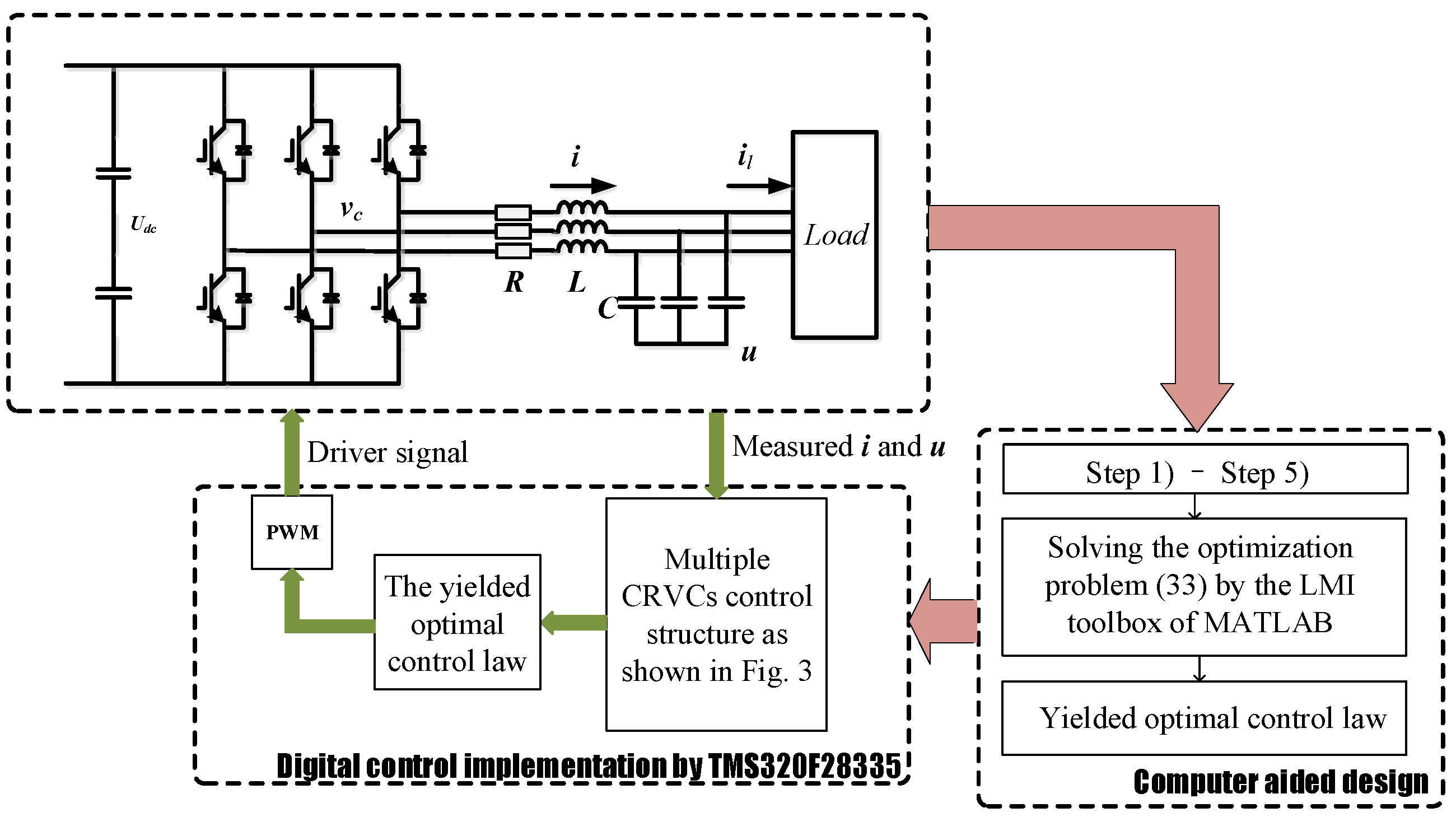
4. Application and Verification

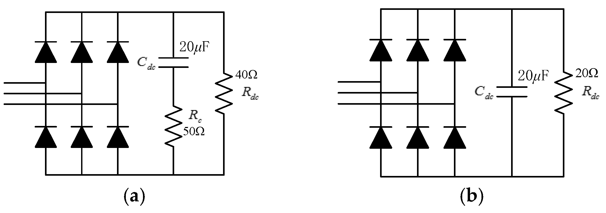
In this section, the proposed control synthesis approach is verified by simulation and experiment. The circuit used in simulation and experiment, a 5 kVA PWM three-phase inverter, is shown in Figure 5. The inverter’s nominal parameters are detailed in

Table 2. Parameters of the three-phase invert.

Variable	Significance	Value
L	Inductance	2 mH
C	Capacitance	30 μF
R	Inductor resistance	0.5 Ω
fs	Switch frequency	12,800 Hz
	Output voltage peak	311 V
	DC link voltage	650 V

. The output voltage and the inductor current are obtained from measurements made possible by a Hall effect sensor, which is used to compose the state feedback control law for performance improvement of the overall system. Furthermore, the load current is unnecessary for the optimal control law.

4.1. Case Study

For the three-phase inverter with the nominal parameters as shown in Table 2, to obtain a low THD for the output voltage, a multiple CRVC structure considering six resonant modes will employ the fundamental positive and negative sequence (n = ±1), twice negative sequence (n = −2), fifth negative sequence (n = −5), seventh positive sequence (n = 7) and 11th negative sequence (n = −11). The design of the multiple CRVCs starts with the selection of a set of the parameters for the LMI region $D\left(\sigma ,r,\theta \right)$. Here we set the parameters as σ = 200, r = 2π × 50 × 13, θ = π/2 such that the transient response of the overall system is approximately one period of the fundamental component. This value is obtained considering the approximation for the settling time t_s = 3/σ. The parameter θ = π/2 means that it does not impose any restriction on the damping ratio [40]. The set of r is considered as an upper bound of the maximum frequency constraint of the non-dominant poles. Then based on the maximum controllable harmonic (controlled by CVRC), which is the 11th harmonic in this paper, the r is set to 2π × 50 × 13 so that the high order harmonics are attenuated effectively. After the parameters are set, solving the convex optimization problem (33) could conveniently yield the different robust optimal state feedback control laws with different combinations of a and b. The consequential control law where a = 1 and b = 1 is shown in

Table 3. Values of the control laws.

Variable	Method in 26	LQR	The Proposed Approach with a = 1, b = 1
$K_{p1}^{\left(i\right)}$	15.8836306685511 − j0.236950325611173	4.97008210384462	6.1118757040980984 − j0.34847163443228379
$K_{p1}^{\left(u\right)}$	0.90564004136966 − j0.0795364207060859	0.328182730006515 − j0.0264301565213812	0.01969918364658270 − j0.1087245143573579
$K_{c1}^{\left(+1\right)}$	−224.980219438506 + j200.222952492662	−98.8992557609345 + j14.7965269551116	−187.17608886575 + j226.78327067540437
$K_{c2}^{\left(-1\right)}$	−318.59139186677 + j244.142045864815	−98.8196531191056 + j15.3191434949775	−312.155066799714 + j236.03740844488078
$K_{c3}^{\left(-2\right)}$	−337.457407096336 − j 193.141886574298	−70.0566409645719 − j9.59515798520183	−291.80188834927043 − j228.45515137729637
$K_{c4}^{\left(-5\right)}$	−285.046690109709 − j7.02975962859623	−69.4806377962434 + j13.1316781649438	−227.27849531760467 − j83.591874218641919
$K_{c5}^{\left(+7\right)}$	−257.199648231256 − j82.264392533777	−64.8801674954042 − j28.1169675777419	−186.70790924243212 + j44.445109123432452
$K_{c6}^{\left(+11\right)}$	−181.365786957522 + j228.403814890761	−23.3264892093487 + j66.7523400426255	−82.369151850982988 + j68.96189605286802

.

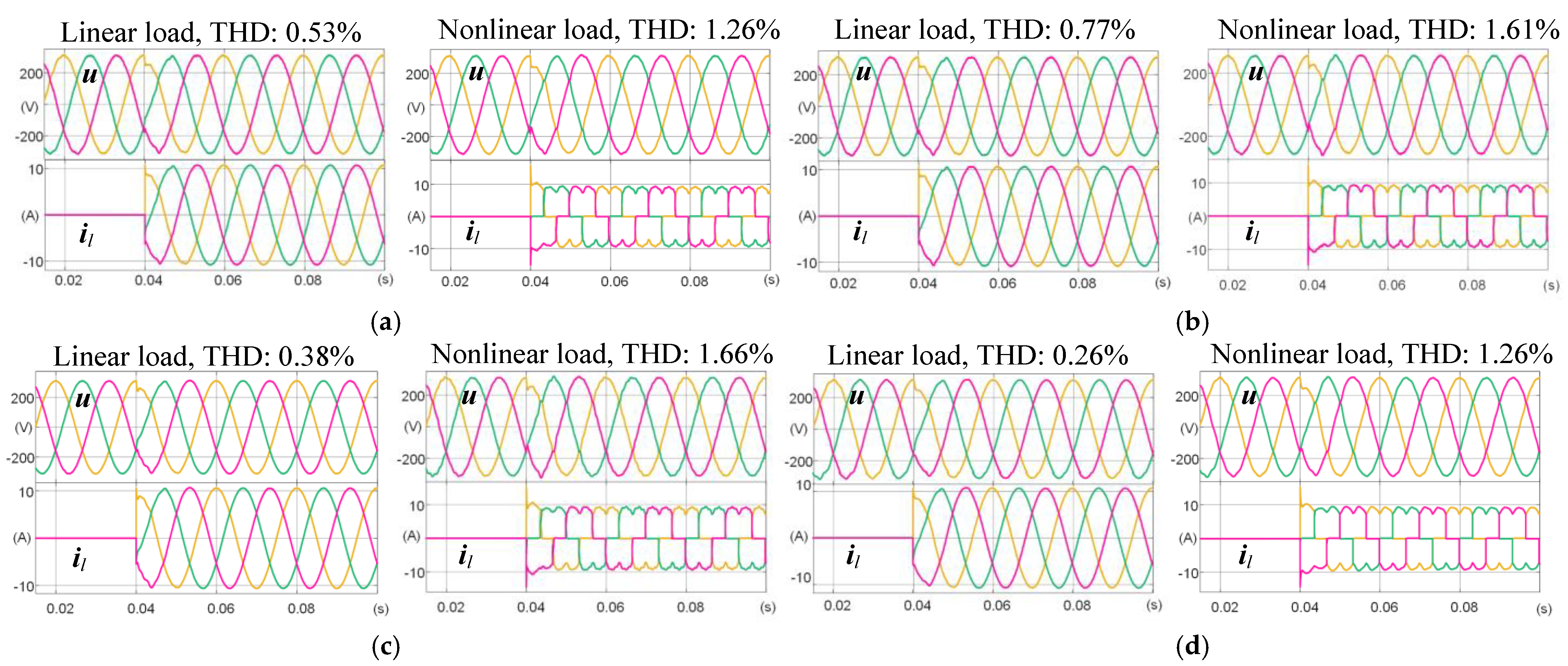
4.2. Simulation Verifications

The proposed optimal control law displayed in Table 3 was performed through simulation with MATLAB/Simulink. To further justify the robustness under parameter variations, the used values of the output filter in the simulation were changed. In those simulation cases as shown in Figure 6, the mutational linear and non-linear loads are used to verify the dynamic and steady performance. The non-linear load for the simulation is shown in Figure 7a where the Rc is used to restrain the overlarge charge current of C_dc in a pure ideal simulation environment. Figure 6 shows the simulation results of the proposed optimal control law for different LC filter parameters. The corresponding voltage THD value in each case is labeled in the figure which proves that the proposed control allows obtaining a lower voltage THD value under different load conditions. Figure 6 also reveals the good dynamic performance and high robustness resulting from the proposed control algorithm in parameter variation.

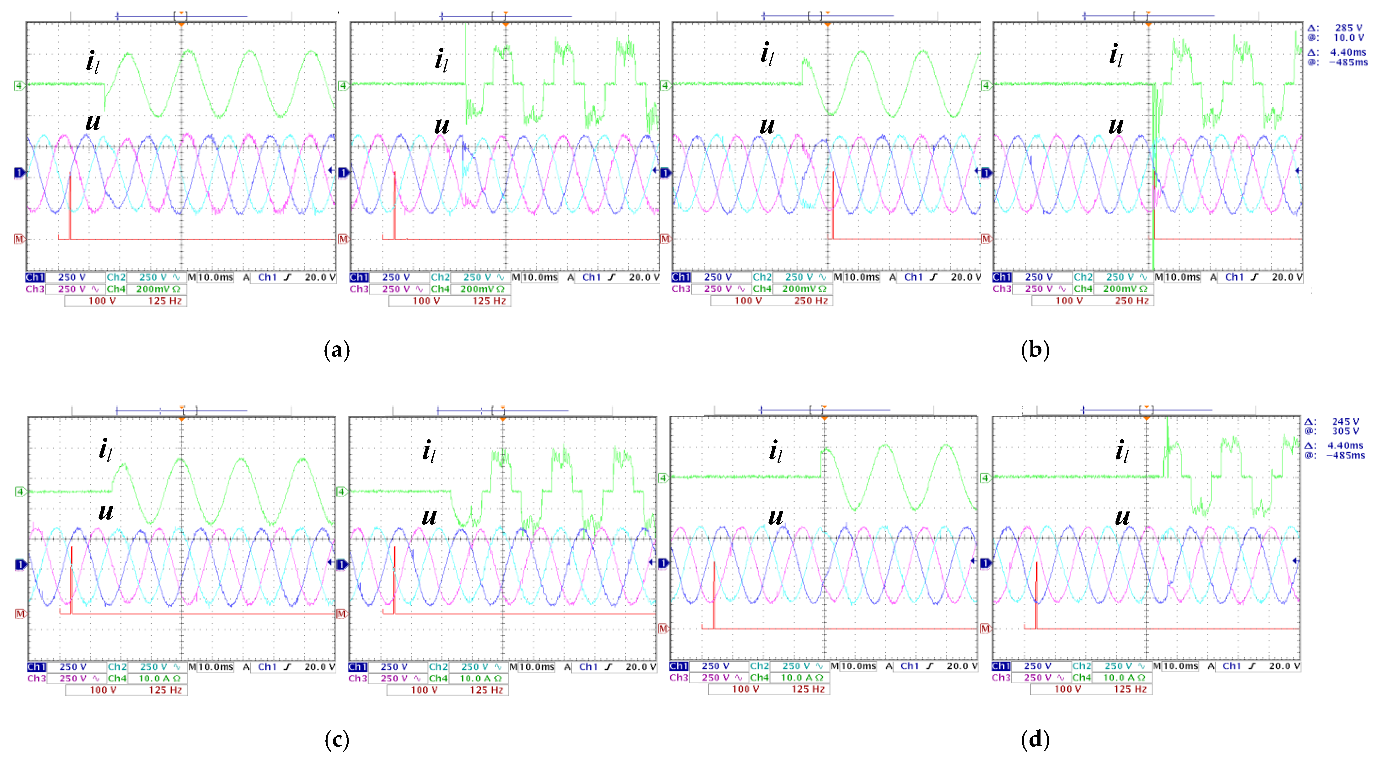
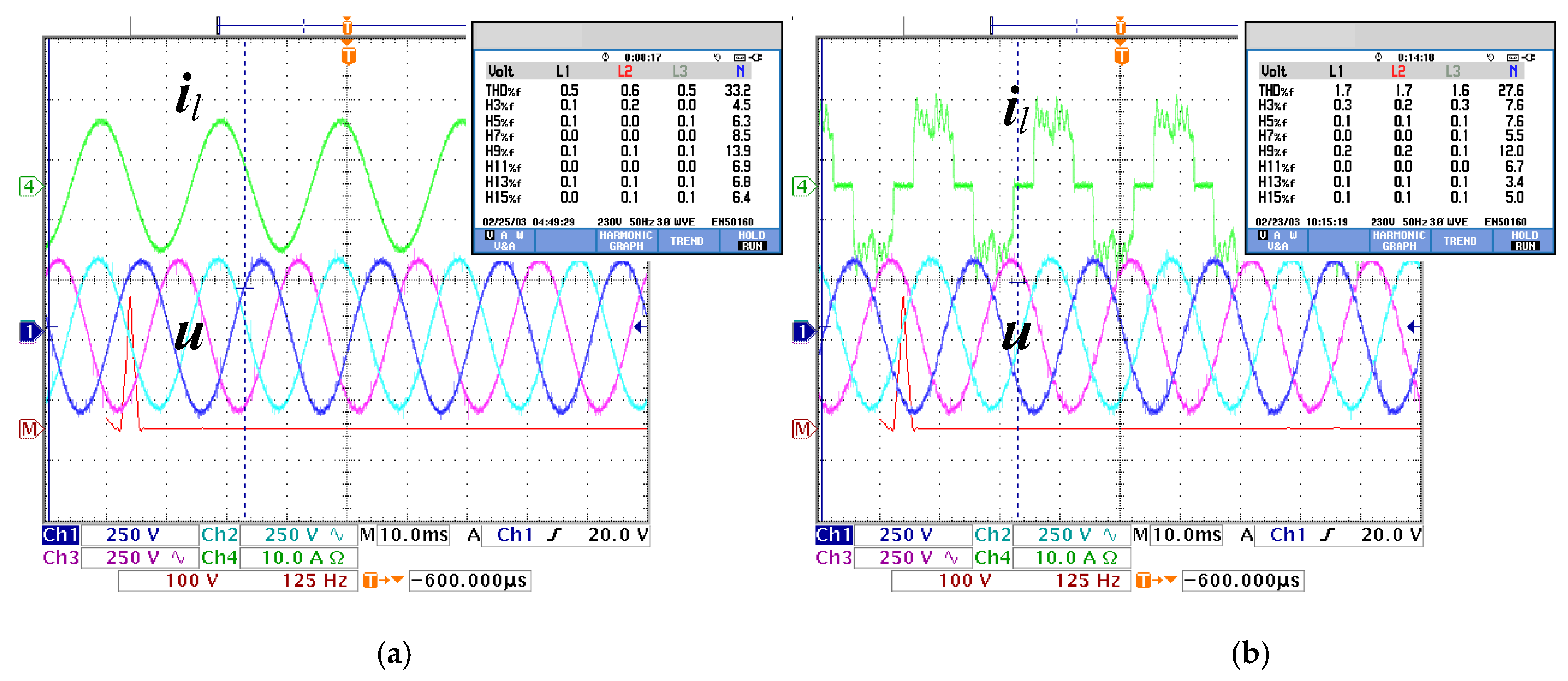
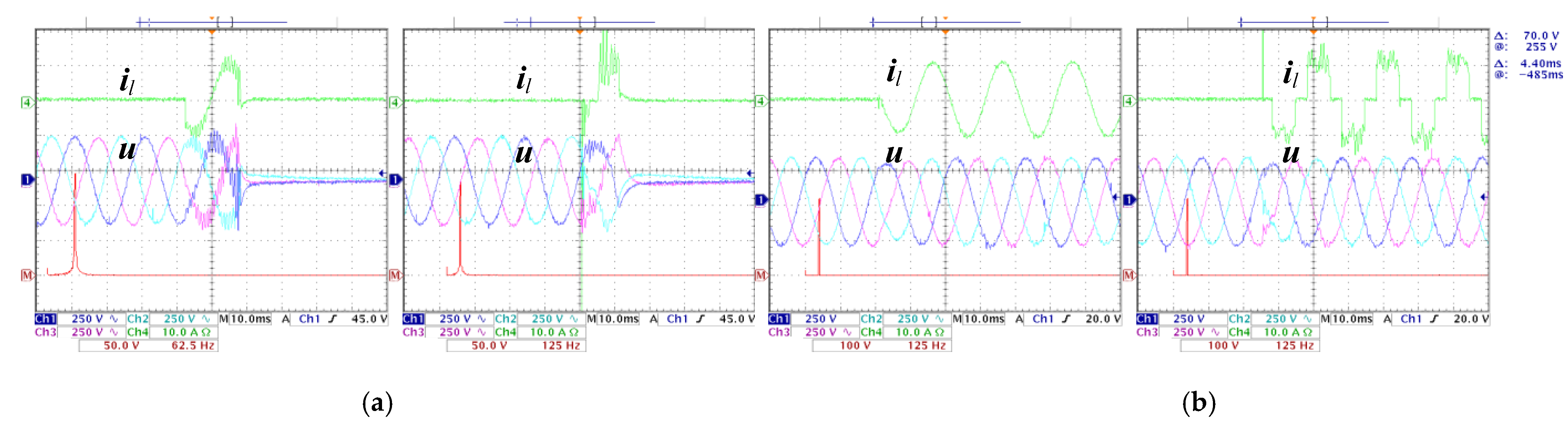
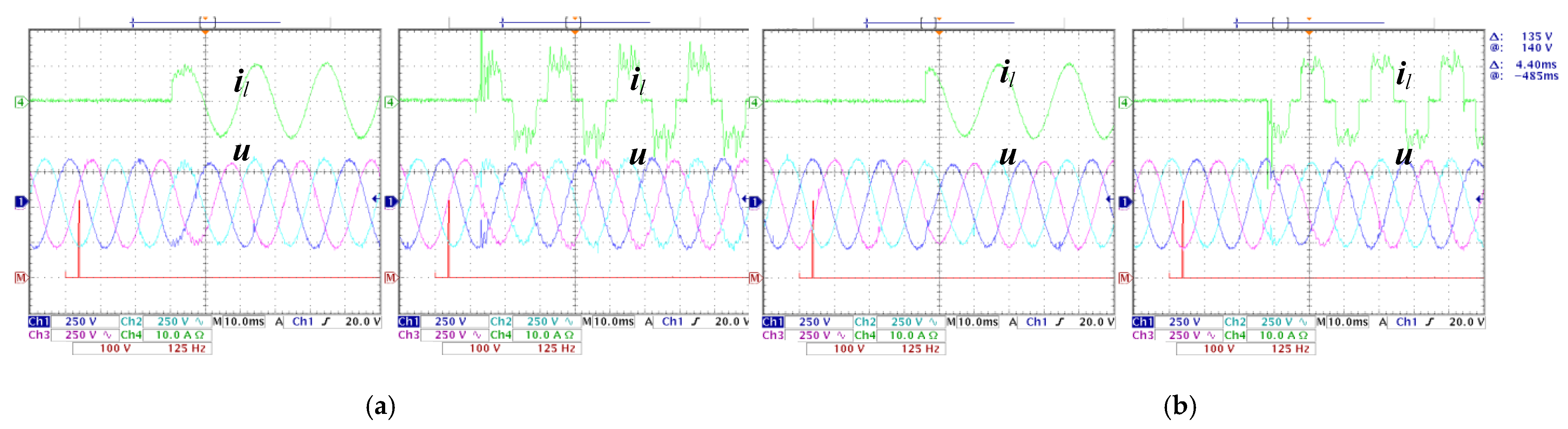
4.3. Experiment Verifications

Some comparative experiment results were conducted to verify the effectiveness and superiority of the proposed control algorithm. Basically, two kinds of load were used: (1) the linear resistor load and (2) the non-linear three-phase diode rectifier load, as shown in Figure 7b. They were used to suddenly connect and disconnect to the inverter to verify both transient response and steady performance. Figure 5 illustrates the schematic of the system and the synoptic diagram of the implemented scheme, which used a 16-bit floating-point TMS320LF28335 DSP. To further justify the robustness under parameter variations, the proposed optimal control law has been tested under different LC filter parameters, which are 1 mH, 30 μF; 2 mH, 15 μF; 2 mH, 30 μF (nominal); and 2 mH, 60 μF. Besides that, the method proposed in [26] is compared in the experimental tests. Moreover, the conventional LQR with the weighting matrix (34), whose control law was calculated by the function lqr() provided by MATLAB, was also compared to highlight the advantages of the proposed optimal control law. The weighting matrix (34), where diag() denotes the diagonal matrix, was selected by trial-and-error method with the assistance of the root locus [34]. All the tested control laws, which were derived directly from the calculation of the aided software without any change, are listed in Table 3.

$$R=\mathrm{diag}\left(0.5 0.5 10000 10000 5000 5000 5000 5000\right)$$

(34)

Firstly, the steady voltage waveforms with different loads, as shown in the Figure 8, are used to analyze the steady THD. The total THD are 0.5% and 1.7% for the linear and non-linear load, respectively. Moreover, based on the analysis of the THD of individual harmonics, we discovered that the 5th, 7th and 11th harmonics are greatly suppressed due to the contribution of the corresponding CVRCs. This implies that the total THD will become lower if more CVRCs are configured. Moreover, the number increasing of the CRVC does not increase the design difficulty of the proposed LMI approach.

In the second group of experiments, the proposed optimal control law was compared to the method in [26] and to the conventional LQR approach with respect to dynamic performance, robustness to parameter variations and THD. Figure 9 shows where dynamic waveforms of the proposed optimal control law are under mutational linear and non-linear load with LC filter parameter variations; furthermore, the proposed optimal control algorithm exhibited high robustness and good dynamic performance regardless of LC filter parameter variations. The best dynamic performance was shown in the nominal parameter (2 mH, 30 μF) as shown in Figure 9c with little fluctuation and fast recovering time for both the mutational linear and non-linear loads. Although the transient process demonstrates some deterioration in other LC filter parameters, it also proved acceptable and consistently stable.

Table 4. Performance comparison of the three control methods for output voltage.

	1 mH, 30 μF		2 mH, 15 μF		2 mH, 30 μF (Nominal)		2 mH, 60 μF
	Linear Load	Nonlinear Load	Linear Load	Nonlinear Load	Linear Load	Nonlinear Load	Linear Load	Nonlinear Load
The proposed approach	Inferior dynamic performance, THD: 2.1% RMS: 220.1 V	Inferior dynamic performance, THD: 1.9% RMS: 220.2 V	Inferior dynamic performance, THD: 0.6% RMS: 220.1 V	Good dynamic performance, THD: 1.8% RMS: 220.1 V	Excellent dynamic performance, THD: 0.5% RMS: 220 V	Excellent dynamic performance, THD: 1.7% RMS: 220.1 V	Good dynamic performance, THD: 0.3% RMS: 220 V	Good dynamic performance, THD:1.4% RMS: 220 V
The method in [26]	Can’t start up *	Can’t start up	Can’t start up	Can’t start up	Instability *	Instability	Inferior dynamic performance, THD: 0.7% RMS: 219.8 V	Inferior dynamic performance, THD: 2.0% RMS: 219.8 V
LQR	Can’t start up	Can’t start up	Instability *	Instability	Inferior dynamic performance, THD: 0.7% RMS: 220 V	Inferior dynamic performance, THD: 3.4% RMS: 220.2 V	Inferior dynamic performance, THD: 0.6% RMS: 219.9 V	Inferior dynamic performance, THD: 2.1% RMS: 220 V

* Can’t start up: Voltage can’t be established even in idle state. Instability: Voltage can be established in idle state, but it is unstable when load is applied suddenly.

summarizes conclusive performance aspects such as stability, voltage THD and dynamic process in each case and in other tested values of parameters.

To illustrate the superiority of the proposed design approach, the method in [26] was tested. The experiment wave shapes are displayed in Figure 10, which only shows the result with LC filter parameters of 2 mH, 30 μF and 2 mH, 60 μF. Because for the parameters of 1 mH, 30 μF and 2 mH, 15 μF, the yielded control law from [26] was not able to start up. Furthermore, in view of the waveforms in Figure 10, the control law from the method in [26] encountered instability when the load was applied suddenly in the nominal parameters. However, for the LC parameters of 2 mH, 60 μF, it worked well. This may be due to its natural properties, which are to minimize the H∞ norm to acquire the maximization of the ability of disturbance rejection without any consideration of the physical limitation of the control input. However, the disturbance rejection ability is positively related to the capacitance of the LC filter. The larger the capacitance, the higher the ability of disturbance rejection is acquired. In the case of this test, the disturbance rejection ability designed by the method of [26] cannot be realized by the nominal LC parameters in this paper so that it appears to be an instability phenomenon. It is worth noting that the capacitance of the LC filter adopted in [26] is 300 μF which is 10 times that of its counterpart in this research. This is why the design approach worked well in [26] and implies that the proposed approach has broader adaptability.

To demonstrate the improvement contribution to the conventional LQR of the proposed optimal LQ control design approach, the conventional LQR was also tested with the same loads and parameter variations. Similarly, while in the condition of 1 mH, 30 μF and 2 mH, 15 μF, the LQR is unstable. Figure 11 shows experimental results for the other LC parameters. Apparently, from Figure 11, the dynamic performance of the conventional LQR is worse than the proposed optimal control law in both tests. Moreover, a few distortions appear in the voltage in the case of a nonlinear load under nominal parameters. Finally, the comprehensive performance comparison is summarized in Table 4, which can demonstrate the superiority of the proposed approach.

5. Conclusions

This paper has proposed an efficient and systematic inverter optimal control design approach by means of an objective-selectable convex optimization problem, which can be perfectly solved by the LMI method. The approach is able to conveniently design the high-dimension parameters for the multiple resonant controller. Besides that, the approach avoids the subjective and time-consuming selection of the high-dimension weighting matrix Q for LQR.

The yielded optimal control law is allowed to optimally compromise several aspects of indexes leading to some excellent control characteristics such as internal stability, outstanding steady and transient response, and disturbance resistance, especially for the abrupt non-linear loads. The simulation and experimental results demonstrated that the proposed optimal control law has excellent performance such as fast recovering time, small fluctuation in load change, low THD and high robustness. Hence, the validity and superiority of the proposed approach were verified.

The main disadvantage of the proposed approach is that some conservativeness is introduced in the design process due to the adopted common optimized variable W. Hence, future work will be mainly to overcome this drawback in order to reduce the conservativeness. The iteration optimization may be a suitable method.

References

1. Zou, Z.; de Carne, G.; Buticchi, G.; Liserre, M. Smart Transformer-Fed Variable Frequency Distribution Grid. IEEE Trans. Ind. Electron. 2018, 65, 749–759. [Google Scholar] [CrossRef]
2. Zou, Z.; Buticchi, G.; Liserre, M. Grid Identification and Adaptive Voltage Control in a Smart Transformer-Fed Grid. IEEE Trans. Power Electron. 2019, 34, 2327–2338. [Google Scholar] [CrossRef]
3. Alhelou, H.H.; Golshan, M.E.H.; Hatziargyriou, N.D. A Decentralized Functional Observer Based Optimal LFC Considering Unknown Inputs, Uncertainties, and Cyber-Attacks. IEEE Trans. Power Syst. 2019, 34, 4408–4417. [Google Scholar] [CrossRef]
4. Haesalhelou, H.; Parthasarathy, H.; Nagpal, N.; Agarwal, V.; Nagpal, H.; Siano, P. Decentralised Stochastic Disturbance Observer-Based Optimal Frequency Control Method for Interconnected Power Systems with High Renewable Shares. IEEE Trans. Ind. Inform. 2021. [Google Scholar] [CrossRef]
5. Quan, X.; Huang, A.Q.; Yu, H. A Novel Order Reduced Synchronous Power Control for Grid-Forming Inverters. IEEE Trans. Ind. Electron. 2020, 67, 10989–10995. [Google Scholar] [CrossRef]
6. Quan, X.; Yu, R.; Zhao, X.; Lei, Y.; Chen, T.; Li, C.; Huang, A.Q. Photovoltaic Synchronous Generator: Architecture and Control Strategy for a Grid-Forming PV Energy System. IEEE J. Emerg. Sel. Top. Power Electron. 2020, 8, 936–948. [Google Scholar] [CrossRef]
7. Loh, P.C.; Newman, M.J.; Zmood, D.N.; Holmes, D.G. A comparative analysis of multiloop voltage regulation strategies for single and three-phase UPS systems. IEEE Trans. Power Electron. 2003, 18, 1176–1185. [Google Scholar]
8. Mohamed, Y.A.R.I.; Radwan, A. Hierarchical control system for robust microgrid operation and seamless mode transfer in active distribution systems. IEEE Trans. Smart Grid. 2011, 2, 352–362. [Google Scholar] [CrossRef]
9. Deng, H.; Oruganti, R.; Srinivasan, D. A simple control method for high-performance UPS inverters through output-impedance reduction. IEEE Trans. Ind. Electron. 2008, 55, 888–898. [Google Scholar] [CrossRef]
10. Kawabata, T.; Miyashita, T.; Yamamoto, Y. Dead beat control of three phase PWM inverter. IEEE Trans. Power Electron. 1990, 5, 21–28. [Google Scholar] [CrossRef]
11. Mattavelli, P. An improved deadbeat control for UPS using disturbance observers. IEEE Trans. Ind. Electron. 2005, 52, 206–212. [Google Scholar] [CrossRef]
12. Escobar, G.; Valdez, A.A.; Leyva-Ramos, J.; Mattavelli, P. Repetitive-based controller for a UPS inverter to compensate unbalance and harmonic distortion. IEEE Trans. Ind. Electron. 2007, 54, 504–510. [Google Scholar] [CrossRef]
13. Jung, S.L.; Tzou, Y.Y. Discrete sliding-mode control of a PWM inverter for sinusoidal output waveform synthesis with optimal sliding curve. IEEE Trans. Power Electron. 1996, 11, 567–577. [Google Scholar] [CrossRef]
14. Komurcugil, H. Rotating-sliding-line-based sliding-mode control for single-phase UPS inverters. IEEE Trans. Ind. Electron. 2012, 59, 3719–3726. [Google Scholar] [CrossRef]
15. Cortés, P.; Ortiz, G.; Yuz, J.I.; Rodríguez, J.; Vazquez, S.; Franquelo, L.G. Model predictive control of an inverter with output LC filter for UPS applications. IEEE Trans. Ind. Electron. 2009, 56, 1875–1883. [Google Scholar] [CrossRef]
16. Yaramasu, V.; Rivera, M.R.; Narimani, M.; Wuet, B.; Rodriguez, J. Model Predictive Approach for a Simple and Effective Load Voltage Control of Four-Leg Inverter with an Output Filter. IEEE Trans. Ind. Electron. 2012, 61, 5259–5270. [Google Scholar] [CrossRef]
17. Do, T.D.; Leu, V.Q.; Choi, Y.S.; Choiet, H.H.; Jung, J. An adaptive voltage control strategy of three-phase inverter for stand-alone distributed generation systems. IEEE Trans. Ind. Electron. 2013, 60, 5660–5672. [Google Scholar] [CrossRef]
18. Jung, J.W.; Vu, N.T.T.; Dang, D.Q.; Doet, T.D.; Choi, Y.; Choi, H.H. A three-phase inverter for a standalone distributed generation system: Adaptive voltage control design and stability analysis. IEEE Trans. Energy Convers. 2014, 29, 46–56. [Google Scholar] [CrossRef]
19. Kim, D.E.; Lee, D.C. Feedback linearization control of three-phase UPS inverter systems. IEEE Trans. Ind. Electron. 2010, 57, 963–968. [Google Scholar]
20. Houari, A.; Renaudineau, H.; Martin, J.P.; Pierfederici, S.; Meibody-Tabar, F. Flatness-based control of three-phase inverter with output filter. IEEE Trans. Ind. Electron. 2012, 59, 2890–2897. [Google Scholar] [CrossRef]
21. Komurcugil, H.; Altin, N.; Ozdemir, S.; Sefa, I. An Extended Lyapunov-Function-Based Control Strategy for Single-Phase UPS Inverters. IEEE Trans. Power Electron. 2015, 30, 3976–3983. [Google Scholar] [CrossRef]
22. Razi, R.; Monfared, M. Simple control scheme for single-phase uninterruptible power supply inverters with Kalman filter-based estimation of the output voltage. IET Power Electron. 2015, 8, 1817–1824. [Google Scholar] [CrossRef] [Green Version]
23. Willmann, G.; Coutinho, D.F.; Pereira, L.F.A.; Líbano, F.B. Multiple-loop H-infinity control design for uninterruptible power supplies. IEEE Trans. Ind. Electron. 2012, 54, 1591–1602. [Google Scholar] [CrossRef]
24. Lim, J.S.; Lee, Y.I. Design of a robust controller for three-phase UPS systems using LMI approach. In Proceedings of the International Symposium on Power Electronics Power Electronics, Electrical Drives, Automation and Motion, Sorrento, Italy, 20 June 2012. [Google Scholar]
25. Lim, J.S.; Park, C.; Han, J.; Lee, Y.I. Robust Tracking Control of a Three-Phase DC–AC Inverter for UPS Applications. IEEE Trans. Ind. Electron. 2014, 61, 4142–4151. [Google Scholar] [CrossRef]
26. Pereira, L.F.A.; Flores, J.V.; Bonan, G.; Gomes da Silva, J.M., Jr. Multiple resonant controllers for uninterruptible power supplies—A systematic robust control design approach. IEEE Trans. Ind. Electron. 2014, 61, 1528–1538. [Google Scholar] [CrossRef]
27. Tarczewski, T.; Grzesiak, L.M. State feedback control of the PMSM servo-drive with sinusoidal voltage source inverter. In Proceedings of the 2012 15th International Power Electronics and Motion Control Conference (EPE/PEMC), Novi Sad, Serbia, 4–6 September 2012; pp. DS2a. 6-1–DS2a. 6-6. [Google Scholar]
28. Hasanzadeh, A.; Edrington, C.S.; Maghsoudlou, B.; Mokhtari, H. Optimal LQR-based multi-loop linear control strategy for UPS inverter applications using resonant controller. In Proceedings of the 2011 50th IEEE Conference on Decision and Control and European Control Conference, Orlando, FL, USA, 12–15 December 2011; pp. 3080–3085. [Google Scholar]
29. Hasanzadeh, A.; Edrington, C.S.; Maghsoudlou, B.; Fleming, F.; Mokhtari, H. Multi-loop linear resonant voltage source inverter controller design for distorted loads using the linear quadratic regulator method. IET. Power Electron. 2012, 5, 5841–5851. [Google Scholar] [CrossRef]
30. Kaszewski, A.; Grzesiak, L.M.; Ufnalski, B. Multi-oscillatory LQR for a three-phase four-wire inverter with L 3n C output filter. In Proceedings of the IECON 2012—38th Annual Conference on IEEE Industrial Electronics Society, Montreal, QC, Canada, 25–28 October 2012; pp. 3449–3455. [Google Scholar]
31. Quan, X. Improved Dynamic Response Design for Proportional Resonant Control Applied to Three-Phase Grid-Forming Inverter. IEEE Trans. Ind. Electron. 2021, 68, 9919–9930. [Google Scholar] [CrossRef]
32. Quan, X.; Dou, X.; Wu, Z.; Hu, M.; Song, H.; Huang, A.Q. A Novel Dominant Dynamic Elimination Control for Voltage-Controlled Inverter. IEEE Trans. Ind. Electron. 2018, 65, 6800–6812. [Google Scholar] [CrossRef]
33. Ufnalski, B.; Kaszewski, A.; Grzesiak, L.M. Particle Swarm Optimization of the Multioscillatory LQR for a Three-Phase Four-Wire Voltage-Source Inverter with an Output Filter. IEEE Trans. Ind. Electron. 2015, 62, 484–493. [Google Scholar] [CrossRef]
34. Quan, X.; Dou, X.; Wu, Z.; Hu, M.; Yuan, J. Harmonic voltage resonant compensation control of a three-phase inverter for battery energy storage systems applied in isolated microgrid. Electr. Power Syst. Res. 2016, 131, 205–217. [Google Scholar] [CrossRef]
35. Kim, E.K.; Mwasilu, F.; Choi, H.H.; Jung, J.W. An Observer-Based Optimal Voltage Control Scheme for Three-Phase UPS Systems. IEEE Trans. Ind. Electron. 2015, 62, 2073–2081. [Google Scholar] [CrossRef]
36. Scherer, C. H control by state feedback: An iterative algorithm and characterization of high-gain occurence. Syst. Control. Lett. 1989, 12, 383–391. [Google Scholar] [CrossRef]
37. Busada, C.A.; Jorge, S.G.; Leon, A.E.; Solsona, J.A. Current controller based on reduced order generalized integrators for distributed generation systems. IEEE Trans. Ind. Electron. 2012, 59, 2898–2909. [Google Scholar] [CrossRef]
38. El Ghaoui, L.; Feron, E.; Balakrishnan, V. Linear Matrix Inequalities in System and Control Theory; Society for Industrial and Applied Mathematics: Philadelphia, PA, USA, 1994. [Google Scholar]
39. Scherer, C.; Weiland, S. Linear Matrix Inequalities in Control; Lecture Notes; Dutch Institute for Systems and Control: Delft, The Netherlands, 2000. [Google Scholar]
40. Chilali, M.; Gahinet, P. H design with pole placement constraints: An LMI approach. IEEE Trans. Autom. Control. 1996, 41, 358–367. [Google Scholar] [CrossRef]
Figure 1. Structure of the simple inverter system.
Energies 15 00365 g001
Figure 2. State space structure of the complex variable resonant controller (CVRC).
Energies 15 00365 g002
Figure 3. Closed-loop control structure of the system.
Energies 15 00365 g003
Figure 4. Region D in complex plane.
Energies 15 00365 g004
Figure 5. The schematic of the studied system.
Energies 15 00365 g005
Figure 6. Simulation results of the proposed optimal control law with different LC filter parameters: (a) 1 mH, 30 μF; (b) 2 mH, 15 μF; (c) 2 mH, 30 μF (nominal); (d) 2 mH, 60 μF.
Energies 15 00365 g006
Figure 7. Non-linear load circuit with a three-phase diode rectifier for (a) simulation and (b) experiment.
Energies 15 00365 g007
Figure 8. Steady waveforms and the total harmonic distortion (THD) of the proposed optimal control law under nominal LC filter parameters (2 mH, 30 μF): (a) linear load, (b) non-linear load.
Energies 15 00365 g008
Figure 9. Dynamic waveforms of the proposed optimal control law with different LC filter parameters: (a) 1 mH, 30 μF; (b) 2 mH, 15 μF; (c) 2 mH, 30 μF (nominal); (d) 2 mH, 60 μF.
Energies 15 00365 g009
Figure 10. Dynamic waveforms of the method proposed in 26 with different LC filter parameters: (a) 2 mH, 30 μF (nominal); (b) 2 mH, 60 μF.
Energies 15 00365 g010
Figure 11. Dynamic waveforms of the conventional linear quadratic regulation (LQR) with different LC filter parameters: (a) 2 mH, 30 μF (nominal); (b) 2 mH, 60 μF.
Energies 15 00365 g011