Impact of Economic Affluence on CO₂ Emissions in CEE Countries

Abstract

There is huge evidence for a relationship between economic growth and environmental degradation. One of the causes of environmental degradation is CO₂ emission which is added to the atmosphere through human activities and excessive industrialization. The aim of this research is to examine the relationship between CO₂ emissions and measures of wealth in countries of Central and Eastern Europe between 2000 and 2019. The paper extends the research on economic affluence by taking into consideration two measures of economic growth, in addition to GDP, the HDI index is included. The basis for the investigation is the EKC concept. All analyses are based on econometric models with GDP and the HDI index as independent variables. The results are not conclusive and there is no one model which best describes the relationship between CO₂ emissions and economic growth. Verification of the models indicates the better fit of models with the HDI index as the measure of affluence. Moreover, the study confirms that the key factors affecting CO₂ emissions are energy consumption per capita which leads to an increase in CO₂ emissions, and renewable energy consumption which reduces CO₂ emissions. Therefore, technological changes and an increase in human awareness of global sustainability are required.

1. Introduction

Climate change, which affects the whole world in various ways, is, among other things, the result of greenhouse gas emissions (GHG). Carbon dioxide (CO₂) accounts for about 80 percent of total greenhouse gas emissions. Other greenhouse gases are emitted in smaller amounts and are not as commonly produced by human activities as CO₂. Research that has been conducted over the years has confirmed that human-caused greenhouse gas emissions are the dominant cause of the increase in the Earth’s average temperature over the past 250 years. It is said that the period from 1983 to 2012 was the warmest 30-year period of the last 1400 years in the Northern Hemisphere [1].

Global warming and climate change are of interest to scientists, environmentalists, as well as politicians. The effects of climate change affect all over the world; therefore, multi-sectoral international action has to be taken. Examples of global agreements on sustainable development and climate change are the Kyoto Protocol (1997), the Paris Agreement (2015), and other treaties undertaken during climate conferences. They promote a coherent vision of sustainable development based on low-carbon technologies and resource efficiency.

Rising CO₂ emissions are largely driven by economic and population growth. It should be noticed that economic growth has been growing steadily for decades, whereas population growth remains more or less the same. It is very important that economic growth has led to poverty reduction [2,3,4,5] but this pace of growth has relied heavily on fossil fuels emitting huge volumes of CO₂.

There is much evidence of the relationship between economic growth and the environment. One of the theoretical approaches of explaining the impact of economic growth on the environment is the environmental Kuznets curve (EKC). This theory has its origins in the research of the American economist Kuznets, who was the first to describe the non-linear relationship between wealth and income inequality [6]. He showed that income inequality tends to increase at an initial stage of development and then begins to fall as the economy develops. This curve with the shape of an inverted letter “U” was implemented by Grossman and Krueger in the early 1990s to describe the relationship between gross domestic product per capita and the level of pollution [7]. Due to the EKC hypothesis, the process of economic growth after achieving a particular threshold point is expected to limit the environmental degradation created in the early stages of development. Stern [8] considers this phenomenon is attributed to the scale effects in the early stages of growth. However, he points out that pure growth in the scale of the economy would result in increasing the level of environmental degradation if countries were unable to change their economic and technological structures.

Due to the limitations and contradictory results of empirical studies related to the EKC concept, this paper investigates the impact of economic affluence on CO₂ emissions using various variables. Different from previous research, the authors do not define economic affluence only as economic growth. It is well known that GDP is insufficient to measure overall economic performance, particularly in the social and environmental fields. The researchers note that the most important limitations include not taking into account the distribution of income and wealth, not evaluating unpriced and intangible services, and overlooking environmental degradation [9,10]. Therefore, we take into account an alternative measure of economic wealth—the Human Development Index (HDI). Sen and Haq are considered to be the pioneers of this index. Their works on income and human needs as a primary objective of development [11,12,13,14] led to the Human Development Index. This index was first published by the United Nations Development Programme in 1990 [15]. The HDI is focused both on income and on social indicators thus it captures various dimensions.

The purpose of the paper is the examination of the relationship between CO₂ emissions and the economic affluence in CEE countries. Different from other works, this paper extends the economic affluence by taking into consideration two measures of economic growth, in addition to GDP, the HDI is included. The authors were governed by the findings that levels of the HDI give a more complete look at the world and are more adequate than the GDP measure of overall well-being [16]. It is because beyond income, on which GDP is focused, the HDI shifts the attention to other development outcomes, such as health and education. Therefore, we have estimated econometric models for two dependent variables and compared the results. The contribution that this study makes to the literature can be viewed from comparing the results for two measures of economic affluence.

Due to the goal of the paper, three research questions were asked:

• How do variables affect CO₂ emissions form in the CEE countries?
• What is the shape of the EKC in the CEE countries?
• Are there differences in model quality for two measures of affluence (GDP per capita and HDI)?

To answer those questions the study was carried in the following stages:

• Analysis of the variables used in the models.
• Model estimation for GDP per capita and additional explanatory variables.
• Model estimation for the HDI index and additional explanatory variables.

2. Literature Review

There are huge empirical investigations of the relationship between economic growth and CO₂ emissions which indicate their positive impact. The EKC is one of the most used methods to examine this relationship. This method is used in many ways. The authors verify the shape of the EKC, test the hypothesis both for single and for multi-country, consider long and short periods, and include additional explanatory variables. They usually use panel or time-series data.

Concerning the shape of the EKC, a good review was made by Kaika and Zervas [17,18]. They collected the results from papers published from 1992 to 2011. The results have been mixed and inconclusive. More studies found that environmental degradation tends to rise monotonically as income grows so there is no turning point. Shafic and Bandyopadhyay [19] were one of the first to examine the EKC relationship. They considered 149 countries in the period 1960–1990 and found them to be monotonically increasing. Similar results were obtained by Richmond and Kaufmann [20], Lim [21], De Bruyn, van den Bergh, and Opschoor [22], Kunnas and Myllyntaus [23], Halicioglu [24], Holtz-Eakin and Selden [25], Agras and Chapman [26], Borghesi [27], Perrings and Ansuategi [28], Azomahou, Laisney, and Van Phu [29], Aslanidis and Iranzo [30], and Iwata, Okada, and Samreth [31]. The positive monotonic impact of CO₂ emissions for economic growth was confirmed for the Netherlands, Germany, the UK, the USA [22], South Korea [21], Finland [23], and Turkey [24]. The inverted-U relationship between environmental degradation and income was confirmed for Sweden [32], France [33], Pakistan [34], China [35], the group of 15 CEE countries [36], and 14 sub-Saharan African countries [37].

Due to the verification of the EKC relationship for individual country-level and for group country-level, a comprehensive comparison was made by Beşe, Friday, Spencer, and Özden [38]. They analyzed the literature of the EKC concept from 2002 to 2020 and indicated the studies which support the EKC hypothesis and those which did not confirm it. The studies were grouped as multi-country, panel countries, and single country. More studies have supported the EKC relationship (4 for multi-country, 13 for panel countries, 16 for single country). Besides the previously mentioned countries, the EKC relationship was positively verified for Algeria [39], Cambodia [40], Iran [41], Malaysia [42], Mongolia [43], and Portugal [44]. The hypothesis of the EKC concept was rejected in 24 studies that have been analyzed by Beşe, Friday, Spencer, and Özden [38]. There was one multi-country study, eight panel studies, and fifteen single-country studies. The EKC relationship was not confirmed among others for Austria [45], Bangladesh [46], and Indonesia [47]. There are also mixed results for the same country. For example, Munir and Khan [48] have confirmed the EKC concept for Pakistan taking into account the period 1980–2010, whereas Hussain, Javaid, and Drake [49] for the period 1971–2006 have rejected this hypothesis. Mixed results were also found for Turkey, Iran, and the USA. In addition to the above studies, the hypothesis of the EKC concept was also rejected both for the individual country level [20,21,22,23,24] and for the group country level [19,20,25,26,27,28,29,30,31]. There are further mixed results for regional areas with different stages of development [50].

Many authors tested the EKC hypothesis taking into account both a long-term and short-term approach. There are no conclusive results. For example, Saboori, Sulaiman, and Mohd in one study [47] confirmed the EKC hypothesis for Malaysia both in the long-run and short-run, whereas in another study [42] it was confirmed only for the long-term. Ahmed and Long [34] found for Pakistan that there is no relationship in the short-term, while for the long-run the hypothesis was confirmed. The relationship was supported both in the short-run and long-run for France [33], Algeria [51], Mongolia [43], Portugal [44], and Turkey [52]. The results are also mixed using data that cover a long time dating back to the first globalization boom in the 19th century [32,53]. Churchill, Inekwe, Ivanovski, and Smyth [53] tested the EKC hypothesis for 20 OECD countries from 1870 to 2014. Taking into consideration the cross-country panel, they found support for a U-shaped EKC. Nonetheless, evidence for the individual country is mixed. There is a traditional inverted U-shaped relationship for five countries, an N-shaped relationship for three countries, and an inverted N-shaped relationship for one. Lindmark [32] previously confirmed the inverted-U trajectory of EKC examining the same period only for Sweden. He pointed out that technological and structural changes are principal forces that may explain the historical EKC pattern. This interpretation is consistent with the concept used by Gordon [54] who considers that the growth phases are associated with technological clusters: electricity, the internal combustion engine, chemical innovations, communication technologies, and computer technology.

A very important issue in the EKC concept is the variables used. Authors usually examine the relationship between CO₂ emissions and GDP but there are also added other explanatory variables. Energy consumption is one of the most frequently added variables. It is well known that energy consumption causes carbon emissions, and the relationship is positive. Environmental degradation is mainly caused by using non-renewable energy consumption; therefore, the exploitation process of fossil energy has to be limited which in turn means the development of renewable energy. There are many studies of renewable and non-renewable energy as explanatory variables to test the EKC hypothesis. The empirical studies state a positive impact of renewable energy consumption on economic growth [55,56,57,58]. Moreover, there is greater ecological awareness on the well-being of countries, which leads to an increase in the level of obtaining energy from renewable sources. Although renewable sources of energy are initially expensive to install, renewable energy is cheaper to use than traditional energy sources. Therefore, the share of renewable energy in production and consumption is constantly rising. It is also due to the increasing cost of the EU emission allowance. The price of emissions allowances traded on the EU ETS has increased from EUR 8 per tonne of CO₂ equivalent at the beginning of 2018 to around EUR 60 in 2021 [59].

It should be noticed that the use of renewable energy largely depends on the effective implementation of government regulations of resource policies. These concern, in particular, the top five carbon-emitting countries which are China, India, Japan, Russia, and the USA. Hussain and Khan [60] have indicated the influence of environment-related technologies and institutional quality as important factors of limiting CO₂ emissions in those countries. Moreover, consumption-based carbon dioxide is also related to the imports and exports of every economy; therefore, the balance of trade should be adjusted in favor of the least carbon emissions. The role of institutional quality is also underlined by Khan, Ali, Dong, and Lie [61]. They found that fiscal decentralization improves environmental quality, and this relationship is strengthened by improvements in the quality of institutions and the development of human capital. He, Adebayo, Kirikkaleli, and Umar [62] confirmed that globalization and financial development improve the quality of the environment.

Another variable that affects the environment is urbanization. The growing urban population has a significant positive effect on CO₂ emissions [63,64]. The higher urban residents’ income and expenditure contribute to the increase in CO₂ emissions both by the higher energy consumption and increases in road and air transportation [65,66,67]. An interesting investigation was made by Hussain, Usman, Khan, Hassan, Tarar, and Sarwar [68]. Their study of Pakistan suggests that if the population is suitably spread, it can help to reduce environmental degradation. This conclusion was based on the examination of the effect of population density on ecological footprints.

Recently, authors have also highlighted the important role of nuclear energy in pollution mitigation. Danish, Ulucak, and Erdogan [69] have shown that nuclear energy is beneficial for the reduction of production-based CO₂, but it does not reduce consumption-based CO₂ emissions that are traded internationally. In turn, the study of consumption-based carbon emissions in Mexico [62] shows that trade openness has no significant impact on environmental quality.

Taking into account the various country-level, different periods, and various factors affecting CO₂ emissions lead to mixed results for the EKC. Many authors question the elements of this concept. The critiques relate to items such as normal distribution of world income [70,71] and different outcomes depending on the pollutant factor [72,73,74]. It should be emphasized that critiques of the EKC concept do not mean it is worthless. There are different stages of development of countries, various environmental regulations, changing consumption patterns. Therefore, the EKC concept cannot be adopted as an appropriate model for every country or every pollutant. Although there are enormous studies of the relationship between economic growth and the environment, this impact has not been explored by using two measures of economic growth.

3. Materials and Methods

One of the main ways of an examination of the relationship between CO₂ emissions and economic growth is using the environmental Kuznets curve concept. Therefore, at the first stage, the EKC was estimated as a baseline. The study was conducted for 19 countries, which are located in Central and Eastern Europe. Due to CEE countries being diverse in the economy, industrialization, internal and international relations, and environmental policy the EKC can have a different shape. It is because different variables may affect environmental changes. Therefore, local pollution has been also taken into account in empirical models. The estimation of the EKC usually uses a quadratic function where a dependent variable is pollution indicators and the independent variable is income level per capita [7,75]. The standard formulation is given by:

$${\mathrm{Y}}_{\mathrm{it}}={\mathsf{\beta }}_0+{\mathsf{\beta }}_1{\mathrm{GDP}}_{\mathrm{it}}+{\mathsf{\beta }}_2{\mathrm{GDP}}_{\mathrm{it}}^2+{\mathsf{\epsilon }}_{\mathrm{it}}$$

(1)

where Y_it—the measure of environmental degradation in country i, at time t, GDP_it—GDP per capita in country i, at time t.

In our study in the first step the long-term relationship between CO₂ emissions and economic growth has been formulated as follows:

$${\mathrm{CO}}_{2\mathrm{it}}={\mathsf{\beta }}_0+{\mathsf{\beta }}_1{\mathrm{GDP}}_{\mathrm{it}}+{\mathsf{\beta }}_2{\mathrm{GDP}}_{\mathrm{it}}^2+{\mathsf{\beta }}_3{\mathrm{EC}}_{\mathrm{it}}+{\mathsf{\epsilon }}_{\mathrm{it}}$$

(2)

where CO_2it—per capita carbon dioxide emissions in metric tons in country i, at time t, EC_it—per capita energy consumption in country i, at time t, β₀, β₁, β₂, β₃—the parameter estimates, ε_it—the error term.

All variables are considered in the natural logarithm.

Model parameters were estimated using the method of least squares. According to the methodological assumptions of the EKC, there are expected β₁ > 0 and β₂ < 0, which means that after reaching some level of welfare an increase in income leads to lower CO₂ emissions. It is because the early stages of economic growth usually mean higher pollution emissions, but beyond some level of income per capita (e.g., it is possible to use better technologies) the trend reverses. This implies the inverted-U shape of the EKC. For the variable EC, it can be assumed that an increase in energy consumption leads to an increase in CO₂ emissions (β₃ > 0).

In the next step, the analysis was extended by including additional explanatory variables into the model (2), which may influence the level of carbon dioxide emissions. Similar to the studies of Shahbaz, Sbia, Hamdi, and Ozturk [63], and Ozturk and Farhani [64] we included urbanization as a factor that significantly affects the increase in CO₂ emissions. The model is presented below:

$${\mathrm{CO}}_{2\mathrm{it}}={\mathsf{\beta }}_0+{\mathsf{\beta }}_1{\mathrm{GDP}}_{\mathrm{it}}+{\mathsf{\beta }}_2{\mathrm{GDP}}_{\mathrm{it}}^2+{\mathsf{\beta }}_3{\mathrm{UR}}_{\mathrm{it}}+{\mathsf{\epsilon }}_{\mathrm{it}}$$

(3)

where UR_it represents the urban population as a percentage of the total population (in country i, at time t).

Our choice was based on the observation that in many countries, especially in developing ones, there is a migration from rural to urban areas. Workers and families decide to migrate usually due to better jobs and socio-economic conditions. The growing urban population has a significant positive effect on CO₂ emissions so it should be β₃ > 0 in Equation (3).

The next variable which has been taken into account is renewable energy consumption. Among others, it has been proposed by Hasnisah, Azlina, and Che [76], and Bölük and Mert [77]. In view of the fact that renewable energy sources have a positive effect on the quality of the environment, we have implanted renewable energy consumption (RE_it) into our model as the percentage of the total final energy consumption in country i at time t. This is given by Equation (4) in which β₃ should be below zero:

$${\mathrm{CO}}_{2\mathrm{it}}={\mathsf{\beta }}_0+{\mathsf{\beta }}_1{\mathrm{GDP}}_{\mathrm{it}}+{\mathsf{\beta }}_2{\mathrm{GDP}}_{\mathrm{it}}^2+{\mathsf{\beta }}_3{\mathrm{RE}}_{\mathrm{it}}+{\mathsf{\epsilon }}_{\mathrm{it}}$$

(4)

Another part of the research was the estimation of models for an alternative approach to the EKC curve. Instead of the explanatory variable GDP, it was proposed to introduce the Human Development Index as the measure of economic affluence [78,79,80]. A mathematical formulation of the HDI is in the Human Development Report [15] (pp. 109). This measure takes into account not only economic income but is also focused on social and economic development related to four criteria: life expectancy at birth, average years of schooling, expected years of schooling, and gross national income per capita. The following models have been formulated:

$${\mathrm{CO}}_{2\mathrm{it}}={\mathsf{\beta }}_0+{\mathsf{\beta }}_1{\mathrm{HDI}}_{\mathrm{it}}+{\mathsf{\beta }}_2{\mathrm{HDI}}_{\mathrm{it}}^2+{\mathsf{\beta }}_3{\mathrm{EC}}_{\mathrm{it}}+{\mathsf{\epsilon }}_{\mathrm{it}}$$

(5)

$${\mathrm{CO}}_{2\mathrm{it}}={\mathsf{\beta }}_0+{\mathsf{\beta }}_1{\mathrm{HDI}}_{\mathrm{it}}+{\mathsf{\beta }}_2{\mathrm{HDI}}_{\mathrm{it}}^2+{\mathsf{\beta }}_3{\mathrm{UR}}_{\mathrm{it}}+{\mathsf{\epsilon }}_{\mathrm{it}}$$

(6)

$${\mathrm{CO}}_{2\mathrm{it}}={\mathsf{\beta }}_0+{\mathsf{\beta }}_1{\mathrm{HDI}}_{\mathrm{it}}+{\mathsf{\beta }}_2{\mathrm{HDI}}_{\mathrm{it}}^2+{\mathsf{\beta }}_3{\mathrm{RE}}_{\mathrm{it}}+{\mathsf{\epsilon }}_{\mathrm{it}}$$

(7)

where HDI_it represents the Human Development Index (in country i, at time t); other markings are the same as in Formulas (2)–(4).

The HDI index is expressed as a number between 0 and 1. The values of variables in the models were transformed into logarithmic values. Therefore, the values of the HDI were negative. Models expressed by Equations (5)–(7) correspond to the classical EKC when β₁ and β₂ have a negative value. The inverted EKC has β₁ > 0 and β₂ > 0. The sign of β₃ should be the same as in the previously described relations.

The Human Development Report published in 2020 explores a metric of a planetary pressures-adjusted Human Development Index which adjusts the standard HDI by a country’s per capita carbon dioxide emissions and material footprint [81]. This is in order to create a new generation of dashboards, as well as metrics for the social costs of carbon or natural wealth. As the gross national income does not account for planetary pressures, it is necessary to take into account changes in total wealth that also include natural capital.

The study was conducted for 19 countries that are located in Central and Eastern Europe and covered the period 2000–2019. The following countries were taken into consideration (we used two-letter country codes according to ISO 3166-1 alpha-2.):

• members of the European Union (11 countries): Bulgaria (BG), Croatia (HR), Czechia (CZ), Estonia (EE), Hungary (HU), Latvia (LV), Lithuania (LT), Poland (PL), Romania (RO) Slovakia (SK), Slovenia (SI),
• candidates for membership of the European Union (4): Albania (AL), North Macedonia (MK), Serbia (RS), Montenegro (ME),
• the potential candidates for membership of the European Union (1): Bosnia and Herzegovina (BA),
• other countries (3): Belarus (BY), Moldova (MD), Ukraine (UA).

The sample included six variables:

• per capita carbon dioxide emissions in metric tons (CO₂),
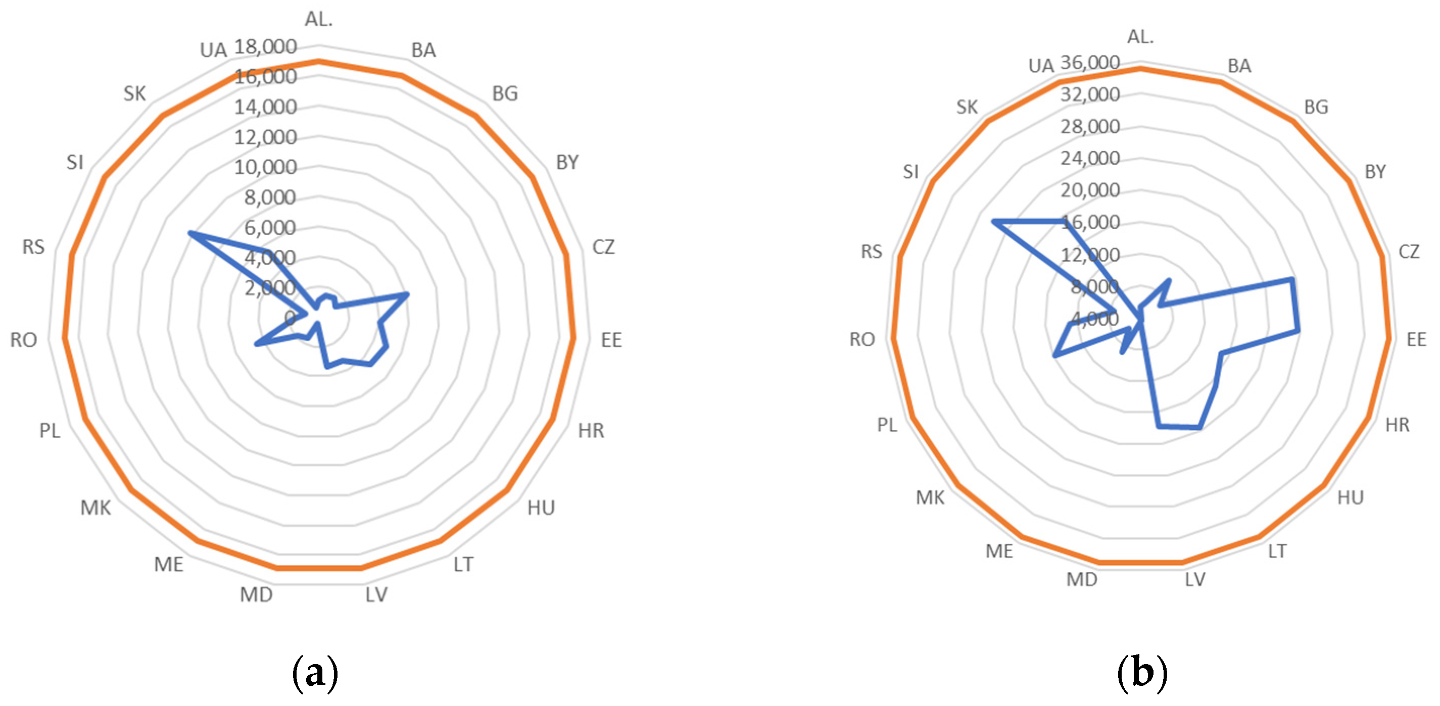
• per capita GDP in constant 2000 USD (GDP),
• energy consumption per capita in a kilogram of oil equivalent (EC),
• urban population as % of total population (UR),
• renewable energy consumption as % of total final energy consumption (RE),
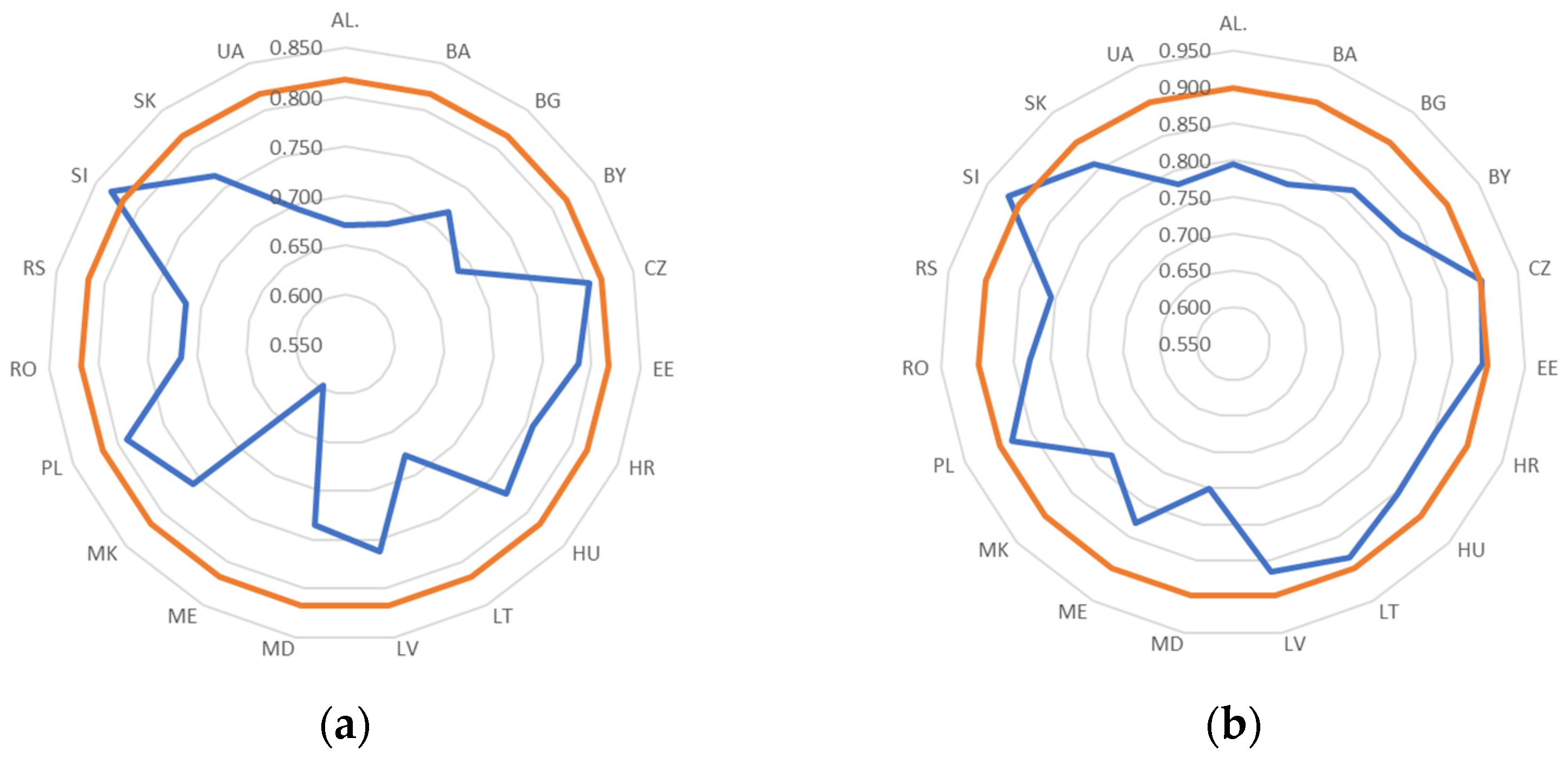
• Human Development Index (HDI).

Data for all sampled countries were obtained from the World Development Indicators of World Bank, Global Change Data Lab (Our World in Data), International Energy Agency, Human Development Report Office, Eurostat, and national statistical institutions. For five countries (AL, BA, MD, ME, and SR) it was not possible to carry out a full analysis because reliable and complete data of energy consumption per capita were not obtained. Therefore, not all models were estimated for those countries. Another limitation of the study was different units of energy measurement which covered different periods. Although standardization of units was made, there was sometimes a lack of consistent time series for the variable EC. Moreover, there were no reliable data for the variable RE in the period 2000–2004.

4. Results

4.1. Analysis of Variables

In the first stage of the research, the analysis of the variables of the models used was carried out. The summary statistics (mean and standard deviation) of CO₂ emissions, energy consumption per capita, per capita GDP, renewable energy consumption, urbanization, and the HDI index are presented in

Table 1. Summary statistics of time-series variables.

Country		CO2	GDP	EC	UR	RE	HDI
AL 1	Mean	1.494	3539.917	906.288	51.538	34.215	0.741
	Stdev	0.280	1284.697	138.861	0.043	2.936	6.073
BY	Mean	6.392	4866.251	2567.174	74.504	6.879	0.772
	Stdev	0.406	2208.787	204.265	2.765	0.474	0.048
BA 1	Mean	5.313	4124.012	1680.100	45.426	22.088	0.732
	Stdev	1.205	1455.258	259.122	1.872	5.528	0.032
BG	Mean	6.444	5995.039	2513.937	72.115	13.554	0.780
	Stdev	0.449	2515.876	120.865	1.970	4.719	0.029
HR	Mean	4.786	11,889.997	1983.886	55.164	25.742	0.812
	Stdev	0.471	3300.369	117.201	1.106	2.217	0.027
CZ	Mean	11.147	16,889.907	4060.595	73.557	10.674	0.861
	Stdev	1.102	5499.941	207.779	0.241	3.604	0.030
EE	Mean	12.754	14,778.992	4319.908	68.601	23.184	0.850
	Stdev	1.368	5954.894	576.366	0.415	4.814	0.030
HU	Mean	5.362	12,125.944	2383.436	68.313	10.432	0.822
	Stdev	0.535	3383.451	135.911	2.310	4.033	0.023
LV	Mean	3.621	11,596.580	1757.453	67.950	34.988	0.821
	Stdev	0.317	4756.507	187.094	0.110	3.278	0.035
LT	Mean	4.346	11,856.599	2158.794	67.001	20.529	0.833
	Stdev	0.447	5024.033	288.016	0.343	3.439	0.033
MD 1	Mean	1.170	2189.125	757.600	42.911	15.791	0.672
	Stdev	0.148	1249.984	86.932	0.586	9.400	0.042
ME 2,3	Mean	3.318	5714.034	1832.256	63.723	39.081	0.792
	Stdev	0.436	2279.740	197.563	2.347	3.617	0.028
MK	Mean	4.471	4151.861	1280.863	57.589	17.210	0.733
	Stdev	0.848	1369.604	70.486	0.447	1.557	0.031
PL	Mean	8.478	10,926.393	2491.483	60.928	9.240	0.837
	Stdev	0.263	3664.852	152.516	0.606	2.049	0.028
RO	Mean	4.367	7476.177	1705.850	53.559	20.494	0.787
	Stdev	0.444	3474.233	89.196	0.439	3.821	0.036
RS 1	Mean	5.445	5144.111	1840.904	54.706	18.845	0.766
	Stdev	0.645	1911.540	112.468	1.072	3.040	0.027
SK	Mean	7.156	14,583.945	3186.007	54.836	9.083	0.822
	Stdev	0.659	4627.136	254.162	0.876	3.154	0.031
SI	Mean	7.756	20,764.041	3460.380	52.584	19.695	0.881
	Stdev	0.748	5177.631	189.768	1.281	2.809	0.023
UA	Mean	6.157	2478.442	2538.227	68.378	3.138	0.750
	Stdev	0.715	1073.697	405.132	0.746	1.968	0.025

¹ EC data are from the period 2000–2016. ² EC data are from the period 2006–2016. ³ RE data are from the period 2005–2019.

.

The average CO₂ emission varied between 1.17 in Moldova and 12.754 in Estonia. The dynamics of CO₂ emissions for all countries are presented in

Table 2. Comparison of emissions of carbon dioxide in 2000 and 2019 (CO₂).

Country	2000 (t Per Person)	EU-28 = 100 (2000)	2019 (t Per Person)	EU-28 = 100 (2019)	2019/2000
AL	0.9602	11.73%	1.9365	21.18%	101.67%
BY	5.5589	67.90%	6.6107	72.32%	18.92%
BA	3.6527	44.62%	8.0646	88.22%	120.78%
BG	5.6645	69.19%	6.0009	65.65%	5.94%
HR	4.4477	54.33%	4.3298	47.37%	−2.65%
CZ	12.3497	150.85%	9.4499	103.38%	−23.48%
EE	10.8965	133.10%	10.4739	114.58%	−3.88%
HU	5.7341	70.04%	5.0698	55.46%	−11.59%
LV	2.9634	36.20%	4.3326	47.40%	46.21%
LT	3.39064	41.42%	4.8853	53.44%	44.08%
MD	0.8502	10.39%	1.4735	16.12%	73.31%
ME	2.47694	30.26%	3.9195	42.88%	58.24%
MK	5.8948	72.01%	3.8605	42.23%	−34.51%
PL	8.2304	100.53%	8.5153	93.15%	3.46%
RO	4.3120	52.67%	3.8773	42.42%	−10.08%
RS	4.7376	57.87%	6.2320	68.17%	31.54%
SK	7.6476	93.42%	6.1050	66.79%	−20.17%
SI	7.7691	94.90%	6.5880	72.07%	−15.20%
UA	5.8425	71.37%	5.0741	55.51%	−13.15%

. Additionally, the values have been compared to the value for European Union countries (EU-28). Taking into account GDP, the richest country is Slovenia, where the average GDP per capita is 20,764.04. There are still considerable differences in the levels of GDP between the countries of Central and Eastern Europe. The data show that the per capita GDP of Moldova and Ukraine is almost 10 times lower than other countries (2189.125 and 2478.442, respectively). The highest consumption of energy is observed in Estonia (4319.908) and the lowest in Moldova (757.6). In the case of urbanization, the highest urban population is in Belarus and the lowest in Moldova. The highest value of renewable energy consumption is achieved by Montenegro (values for the period 2005–2019), Latvia, and Albania. The lowest value of this variable is observed for Ukraine and Belarus. Taking into account the HDI measure, Slovenia is rated the highest and Moldova the lowest.

The highest increase of CO₂ consumption in 2019 compared to 2000 is noted for Bosnia and Herzegovina (120.78%) and Albania (101.67%). On the other hand, North Macedonia (34.51%), the Czech Republic (23.48%), and Slovakia (20.17%) have achieved the largest decrease. In comparison, in the European Union in this time there has been an increase of per capita CO₂ by 9.19%. It should also be noted that most CEE countries have lower CO₂ emissions than EU countries. Only three countries had emissions higher than the EU average in 2000: the Czech Republic (150.85%), Estonia (133.10%), and Poland (100.53%). It is because the level of emissions depends on the size of the country and its industrialization [82]. The lowest emissions are in the least industrialized countries. In this study, it was for Moldova and Albania, where CO₂ emissions in 2000 were ten times lower than in the EU countries.

In 2019, the Czech Republic and Estonia had still a level of emission above the EU average, but their shares were significantly decreased. For eight countries (AL, BY, BA, LV, LT, MD, ME, RS) the share of emissions to the EU average was higher in 2019 than in 2000 but the level of emission was still lower than in the EU. The results give a general view of the carbon dioxide intensity in each country. The emission depends on many factors such as the human population, industry, transportation, energy structure, coal mining, forestry, water management, and national regulations.

Since the goal of this study is to investigate the impact of economic affluence on CO₂ emissions, there is also a detailed analysis of the per capita GDP and the HDI.

There is a huge diversity of CEE countries on the GDP base. The range of values is very wide and varies from USD 440.7 to USD 10,201.3 in 2000. In 2019 the GDP increased significantly in all countries and was between USD 3662.6 and USD 25,940.73. Either in 2000 or 2019, Moldova and Ukraine were the poorest countries, while Slovenia was the richest. In particular, the countries that have been accepted to the European Union since 2004 have denoted significant economic growth. Figure 1 presents the GDP for examined countries in comparison to the value for EU-28.

As in the case of GDP, the differences of the HDI index across the CEE countries are quite large, ranging from the highest value for Slovenia (0.832 in 2000 and 0.917 in 2019) to the lowest for Moldova (0.597 in 2000 and 0.750 in 2019). Slovenia is also the only country of the examined group that had a higher HDI index than the average score in the EU-28 in both years under consideration. Additionally, the Czech Republic recorded the index higher than the EU-28 average in 2019. Estonia and Poland were also close to the EU average. The values of the HDI index are presented in Figure 2.

4.2. Model Estimation

Before the model estimation, the relationship between CO₂ emissions and the other variables was examined. Values of the Pearson correlation coefficient for each country are shown in

Table 3. Pearson correlation coefficient for the CEE countries.

	AL	BY	BA	BG	HR
r(CO2; GDP)	0.885201 *	0.828177 *	0.925366 *	0.208450	−0.084915
r(CO2; HDI)	0.914076 *	0.725106 *	0.904539 *	0.182590	−0.547683 *
	CZ	EE	HU	LV	LT
r(CO2; GDP)	−0.732543 *	0.497535 *	−0.558863 *	0.809403 *	0.912521 *
r(CO2; HDI)	−0.896779 *	0.448619 *	−0.738188 *	0.820451 *	0.894294 *
	MD	ME	MK	PL	RO
r(CO2; GDP)	0.823722 *	0.697156 *	−0.932221 *	0.547932 *	−0.539994 *
r(CO2; HDI)	0.906683 *	0.526670 *	−0.952419 *	0.448910 *	−0.595080 *
	RS	SK	SI	UA
r(CO2; GDP)	−0.103545	−0.745433 *	−0.296614	0.089809
r(CO2; HDI)	−0.253325	−0.887046 *	−0.564192 *	−0.326352

* Correlation coefficients significant at p < 0.05.

.

The correlation coefficient is statistically significant (except BG, RS, and UA for both measures of affluence and HR and SI for GDP) for most countries. The CEE countries by the correlation coefficient between CO₂ and GDP per capita can be grouped as follows:

• a week positive or negative correlation: BG, HR, RS, SI, and UA
• a strong positive correlation: AL, BY, BA, LV, LT, and MD
• a moderately positive correlation: EE, ME, and PL
• a strong negative correlation: CZ, MK, and SK
• a moderately negative correlation: HU and RO

Similar results were obtained for the HDI index as the measure of economic growth. The strength and direction of a correlation coefficient for each country overlapped with those for the GDP. Exceptions were Croatia and Slovenia for which the strength of the relationship was higher in the negative direction. It was mainly due to the CO₂ reduction activities carried out.

The next step was the estimation of the classical EKC for each country. The results using Formulas (2)–(4) are presented in

Table 4. Estimation of model parameters for independent variables GPD and EC.

Country	β0	β1	β2	β3	R2
BY	−3.8227 * (1.0274)	0.5807 ** (0.2622)	−0.0327 *** (0.0160)	0.3972 * (0.0921)	0.93606
BG	−12.2410 * (2.8868)	1.7312 ** (0.7055)	−0.1034 ** (0.0423)	0.8808 * (0.2261)	0.68992
HR	−14.1071 (12.2178)	1.4147 (2.7332)	−0.0801 (0.1500)	1.2451 * (0.2610)	0.60966
CZ	−1.7454 (3.9466)	−1.6502 (0.9505)	0.0813 (0.0506)	1.5033 * (0.1436)	0.94366
EE	−18.1936 * (5.2562)	2.5880 ** (1.0461)	−0.1484 ** (0.0572)	1.1460 * (0.2094)	0.76823
HU	−19.3991 * (4.1040)	2.3893 ** (0.8949)	−0.1384 ** (0.0492)	1.3953 * (0.1020)	0.94639
LV	−0.9339 (4.0207)	−0.2892 (0.9511)	0.0194 (0.0523)	0.4323 *** (0.2053)	0.76754
LT	−0.6179 (2.8125)	0.0731 (0.6713)	0.0067 (0.0374)	0.1084 (0.0745)	0.90276
MK	−2.5668 (8.4996)	−0.6642 (2.4173)	0.0150 (0.1493)	1.1890 * (0.3170)	0.91944
PL	−11.6063 * (2.9209)	1.6282 ** (0.5610)	−0.0941 * (0.0312)	0.8625 * (0.1382)	0.81244
RO	−11.5834 * (2.2614)	0.6404 (0.5872)	−0.0418 (0.0348)	1.4332 * (0.2030)	0.86047
SK	−13.5409 * (4.0473)	1.3127 (0.9579)	−0.0698 (0.0521)	1.1594 * (0.1284)	0.93849
SI	−26.1045 ** (11.3396)	3.2391 (2.3012)	−0.1717 (0.1183)	1.5869 * (0.1616)	0.87174
UA	−5.4008 * (0.8118)	0.3300 (0.2043)	−0.0173 (0.0137)	0.7287 * (0.0224)	0.98545

Due to the incomplete database, models were not estimated for AL, BA, MD, ME, and RS. */**/***—significance level 0.01/0.05/0.1. (…)—standard error.

,

Table 5. Estimation of model parameters for independent variables GPD and UR.

Country	β0	β1	β2	β3	R2
AL	−7.1935 (8.1423)	0.6492 (1.8960)	−0.0356 (0.1245)	1.1847 ** (0.4342)	0.85989
BY	1.3929 (1.4179)	0.9123 * (0.2560)	−0.0478 * (0.0159)	−0.8836 * (0.2222)	0.93048
BA	6.9374 (10.0076)	−3.5833 *** (1.8695)	0.2429 *** (0.1199)	2.0167 *** (1.0310)	0.93578
BG	3.8459 (9.4430)	1.6233 (1.0964)	−0.0893 (0.0685)	−2.1766 (1.4711)	0.46861
HR	12.4571 (10.3489)	2.6680 (2.1018)	−0.1338 (0.1156)	−6.0164 * (0.8705)	0.76270
CZ	23.8731 (33.3701)	2.8160 (2.2767)	−0.1602 (0.1202)	−7.8385 (6.5298)	0.59439
EE	39.8289 (28.2723)	−0.0189 (1.9148)	0.0035 (0.1028)	−8.8519 (5.2915)	0.43359
HU	27.4679 ** (10.5822)	−1.9865 (2.0018)	0.1194 (0.1114)	−4.1838 * (0.7211)	0.78085
LV	−51.5471 (38.6341)	1.1377 (1.1286)	−0.0562 (0.0630)	11.1712 (8.4860)	0.73213
LT	−2.0943 (19.0148)	0.5068 (1.1159)	−0.0180 (0.0627)	0.0978 (3.5202)	0.88990
MD	56.4913 *** (28.6774)	−2.3441 (1.5653)	0.1580 (0.1015)	−12.6979 *** (6.0992)	0.79852
ME	−0.0820 (10.4956)	0.9963 (1.7728)	−0.0449 (0.1077)	−0.9504 (1.8333)	0.55287
MK	−20.3863 (35.1742)	5.4250 (4.2506)	−0.3611 (0.2594)	0.4320 (4.8474)	0.84869
PL	−3.5842 (5.9508)	0.6195 (1.1276)	−0.0310 (0.0630)	0.6448 (1.4541)	0.36352
RO	83.4661 * (19.4327)	1.0182 (0.7499)	−0.0494 (0.0458)	−21.8817 * (4.5744)	0.76365
RS	17.6551 (14.3933)	1.2709 (1.3259)	−0.0687 (0.0857)	−5.4432 *** (2.8551)	0.34599
SK	−32.3297 * (4.8846)	1.5408 (1.1233)	−0.0796 (0.0613)	6.7051 * (0.9095)	0.91471
SI	30.1472 ** (11.0311)	−1.4387 (2.1795)	0.0869 (0.1123)	−5.6507 * (0.5357)	0.88672
UA	78.0534 * (4.2287)	0.4860 (0.3639)	−0.0122 (0.0242)	−18.7589 * (1.0380)	0.95435

*/**/***—significance level 0.01/0.05/0.1. (…)—standard error.

and

Table 6. Estimation of model parameters for independent variables GPD and RE.

Country	β0	β1	β2	β3	R2
AL	9.4834 (14.0318)	−2.6272 (3.2289)	0.1906 (0.2046)	−0.1022 (0.4638)	0.79532
BY	−2.1365 (1.5243)	0.8509 *** (0.4058)	−0.0474 *** (0.0247)	0.1078 (0.1576)	0.86569
BA	20.1582 ** (7.8406)	−5.1782 ** (1.9337)	0.3523 ** (0.1211)	0.0543 (0.5792)	0.92205
BG	−2.6903 (3.7932)	1.0630 (0.9164)	−0.0545 (0.0565)	−0.2117 * (0.0720)	0.60769
HR	−3.6961 (4.6197)	1.9458 *** (1.0101)	−0.1085 *** (0.0555)	−1.0608 * (0.0655)	0.94556
CZ	−2.0087 (1.7379)	1.0513 ** (0.3703)	−0.0536 ** (0.0198)	−0.3159 * (0.0127)	0.98893
EE	−1.4353 (10.1792)	0.7954 (2.1742)	−0.0355 (0.1194)	−0.1169 (0.1708)	0.35346
HU	2.8061 (6.7352)	−0.2289 (1.4872)	0.0185 (0.0822)	−0.2708 * (0.0340)	0.86270
LV	1.9802 (5.6828)	−0.2031 (1.2015)	0.0192 (0.0671)	−0.1300 (0.1541)	0.71576
LT	2.6045 (3.3787)	−0.3743 (0.7295)	0.0330 (0.0411)	−0.1699 *** (0.0870)	0.91108
MD	−0.7644 (2.0152)	0.0648 (0.5647)	0.0135 (0.0404)	−0.1304 ** (0.0537)	0.81287
MK	−11.8121 (9.9340)	3.9696 (2.4194)	−0.2694 *** (0.1496)	−0.3776 *** (0.2124)	0.87359
PL	3.4752 (4.8377)	−0.3381 (1.0695)	0.0233 (0.0596)	−0.0951 *** (0.0463)	0.49018
RO	−3.0435 (2.2556)	1.4998 ** (0.5244)	−0.0798 ** (0.0315)	−0.8236 * (0.1110)	0.87073
RS	5.3976 (4.3410)	−0.5218 (1.0360)	0.0341 (0.0649)	−0.5960 * (0.1245)	0.67008
SK	−10.3693 (6.6811)	2.7494 *** (1.4509)	−0.1466 *** (0.0790)	−0.2470 * (0.0518)	0.84527
SI	−15.0969 (22.4748)	3.7527 (4.6308)	−0.1819 (0.2375)	−0.7297 * (0.2101)	0.48628
UA	3.3064 (1.9506)	−0.5734 (0.5263)	0.0531 (0.0353)	−0.2571 * (0.0217)	0.89996

Due to the incomplete database, the model was not estimated for ME. */**/***—significance level 0.01/0.05/0.1. (…)—standard error.

. Not all estimated parameters are statistically significant. A goodness-of-fit measure for most models is above 0.8. However, a good fit model with statistically insignificant parameters may be caused by the presence of multicollinearity. The sign of the parameters in most models is consistent with expectations (β₁ > 0 and β₂ < 0).

For the above model, there is an inverted-U relationship between CO₂ emissions and GDP per capita for 10 of the 14 investigated countries. It confirms the hypothesis of the presence of the EKC over the studied period. For three countries (CZ, LV, and MK) the estimated parameters had opposite signs (β₁ < 0 and β₂ > 0). In the case of Lithuania, parameters β₁ and β₂ are positive, but after excluding the EC, the signs of the parameters were consistent with the classical EKC (β₁ > 0 and β₂ < 0, R² = 0.70311). It should be noted that for all countries the parameter β₃ was above zero and only for Lithuania was statistically insignificant. This confirms that the increase in energy consumption is a significant factor in rising CO₂ emissions.

Including the variable UR instead of EC has led to the fit of most models being much worse (see Table 5).

For 14 countries the hypothesis of the existence of the classical EKC has been confirmed, while for 5 countries there was an inverted shape of the EKC. Due to the fact that increasing urban population leads to the growth of environmental deterioration and increased CO₂ emissions especially in developing countries, parameter 3 should be positive. The study results confirmed it only for seven countries (AL, BA, LV, LT, MK, PL, and SK). The remaining 12 countries have noted a negative relationship between urbanization and carbon emissions. Statistical significance of urbanization was observed only for 10 models.

The next model included renewable energy consumption as an additional independent variable. The results are presented in Table 6.

The estimated models by Formula (5) were the most varied due to the direction of influence of explanatory variables. Signs consistent with the classical EKC were obtained for nine countries (BY, BG, HR, CZ, EE, MK, RO, SK, and SI), while in eight cases the sign of the GDP per capita indicates the inverted shape EKC. Both parameters (β₁ and β₂) were positive for Moldova. The sign of the effect of renewable energy consumption on CO₂ emission is negative (except BY and BA), which is consistent with the theory. This parameter was statistically significant for 13 countries.

To summarize the first group of models with GDP as the measure of affluence the following models were selected due to the model quality and significance of parameters:

• models with the variable EC: BY, BG, EE, HU, LV, PL, UA,
• models with the variable UR: AL, BA, ME, SI,
• models with the variable RE: HR, CZ, LT, MD, MK, RO, RS, SK.
• Except for Montenegro for which there was a lack of partial information on the explanatory variables, the additional explanatory variables are statistically significant in all models. Therefore, the model for ME should not be included in comparative analyses.
• Due to the hypothesis of the EKC concept, the results of the study are as follows:
• traditional inverted U-shaped EKC (β₁ > 0 and β₂ < 0): AL, BY, BG, HR, CZ, EE, HU, MD, MK, PL, RO, SK, and UA,
• the inverted EKC (β₁ < 0 and β₂ > 0): BA, LV, LT, RS, and SI.

The same analysis was carried for the HDI index instead of GDP as the measure of affluence.

Table 7. Estimation of model parameters for independent variables HDI index and EC.

Country	β0	β1	β2	β3	R2
BY	−1.5076 ** (0.6501)	−4.0894 * (1.2211)	−8.1734 * (2.2853)	0.3674 * (0.0945)	0.93967
BG	−7.1138 * (1.4598)	−12.9348 * (3.4645)	−24.7306 * (6.6885)	0.9353 * (0.1906)	0.77217
HR	−5.8302 * (1.3121)	−18.4043 * (4.7014)	−39.9127 * (10.7850)	0.7028 * (0.1984)	0.83793
CZ	−5.0621 * (1.6297)	−3.4714 (2.7486)	−5.0874 (8.1116)	0.8508 * (0.2187)	0.95835
EE	−9.5357 * (1.1916)	−10.9128 * (2.4698)	−22.8655 * (7.2565)	1.3074 * (0.1358)	0.90410
HU	−8.1947 * (0.6796)	−6.5568 ** (2.5665)	−11.3102 *** (6.1373)	1.1610 * (0.0917)	0.96324
LV	−1.6039 (1.8216)	1.1127 (2.4532)	0.8174 (5.5766)	0.4117 *** (0.2320)	0.75599
LT	1.3775 ** (0.6452)	−0.5255 (2.4917)	−7.5383 (6.2016)	0.0333 (0.0927)	0.83896
MK	−5.5189 * (1.5331)	−0.8145 (6.3576)	4.8822 (9.8252)	0.8754 * (0.2595)	0.93861
PL	−5.4329 * (0.7594)	−0.8157 (0.9970)	0.9194 (2.8700)	0.9456 * (0.0961)	0.89359
RO	−8.0785 * (1.2383)	−9.8266 ** (3.4598)	−16.9977 ** (6.6225)	1.1025 * (0.1970)	0.90348
SK	−5.5641 * (1.0449)	−8.6309 * (1.9738)	−19.7172 * (4.4164)	0.8197 * (0.1449)	0.96582
SI	−8.6577 * (1.2959)	−7.2446 ** (3.2427)	−21.4275 *** (11.7117)	1.2447 * (0.1711)	0.89718
UA	−4.2119 * (0.3179)	2.0058 (2.8984)	0.6924 (4.6092)	0.8361 * (0.0385)	0.98331

Models were not estimated for AL, BA, MD, ME, and RS. */**/***—significance level 0.01/0.05/0.1. (…)—standard error.

,

Table 8. Estimation of model parameters for independent variables HDI index and UR.

Country	β0	β1	β2	β3	R2
AL	−3.4418 (4.2999)	−2.9299 (4.8954)	−6.7448 (7.4620)	0.9090 (0.9416)	0.85739
BY	0.1535 (3.1059)	−7.7535 * (1.8327)	−15.1065 * (2.8164)	0.1776 (0.6667)	0.88316
BA	−32.7913 * (10.6889)	−15.0880 *** (7.2167)	−19.4179 *** (10.2632)	8.2960 * (2.5567)	0.91375
BG	3.4569 (21.0923)	−14.9477 (13.2641)	−30.5295 (20.0260)	−0.7906 (4.4756)	0.43029
HR	−36.3276 (22.2169)	−44.9091 * (12.4480)	−89.8985 * (22.7959)	8.1137 (5.1644)	0.74948
CZ	−36.4644 ** (13.7465)	−17.9107 * (2.5491)	−49.1384 * (8.2551)	8.6898 ** (3.1661)	0.94489
EE	42.0575 (28.7916)	−0.7672 (9.4116)	−3.7041 (28.6609)	−9.3511 (6.6803)	0.41985
HU	33.7281 * (10.1683)	15.7523 (11.3810)	24.4337 (22.7062)	−7.0847 * (2.1191)	0.76167
LV	−39.9411 (56.8399)	−1.3891 (4.7167)	−6.7472 (10.4098)	9.7723 (13.3724)	0.71739
LT	30.4778 (42.5414)	5.0228 (8.9917)	5.3122 (20.9317)	−6.7259 (9.9068)	0.84220
MD	66.1831 ** (25.6664)	18.7780 ** (8.2711)	24.7552 *** (11.7379)	−16.6482 ** (6.4706)	0.89353
ME	−17.8097 ** (7.6362)	−20.9484 (15.0088)	−40.1392 (29.4113)	3.9351 ** (1.5099)	0.40622
MK	−41.0308 (26.6563)	−37.5526 *** (17.7634)	−53.1107 ** (28.3682)	8.8972 (5.9470)	0.90784
PL	−2.5454 (17.2046)	−1.6326 (3.2537)	−6.6630 (7.5281)	1.1220 (4.2550)	0.25286
RO	49.4040 *** (24.2190)	−15.7895 * (5.0450)	−32.1203 * (8.7510)	−12.5117 *** (5.9616)	0.77621
RS	58.5526 (46.3175)	−4.2505 (0.7554)	−20.5096 (23.8631)	14.1208 (11.2294)	0.16729
SK	−14.9979 (12.9340)	−8.7998 (5.7985)	−20.0066 *** (11.1367)	4.0042 (3.3906)	0.90567
SI	32.8537 * (5.4294)	3.8079 (5.0429)	−2.4314 (15.6128)	−7.6440 * (1.2887)	0.86151
UA	75.3950 *** (40.4985)	−8.7087 (19.4835)	−21.6880 (28.0350)	−17.5788 *** (8.8969)	0.59176

*/**/***—significance level 0.01/0.05/0.1. (…)—standard error.

and

Table 9. Estimation of model parameters for independent variables HDI index and RE.

Country	β0	β1	β2	β3	R2
AL	7.1979 * (2.1442)	17.6159 ** (7.0429)	23.8385 *** (11.4832)	−1.0639 * (0.3369)	0.90702
BY	0.9480 * (0.2459)	−7.2183 * (1.5815)	−14.2866 * (2.9808)	0.0267 (0.1558)	0.88285
BA	2.6181 (2.5149)	−0.4275 (12.6822)	−8.6957 (19.4310)	−0.0770 (0.1903)	0.85845
BG	4.8421 * (1.3239)	7.8207 (7.0735)	5.1372 (11.7499)	−0.5332 * (0.1290)	0.72386
HR	4.6680 * (0.8989)	−0.8871 (4.5063)	−1.2857 (10.1341)	−0.9970 * (0.1397)	0.93087
CZ	2.9487 * (0.1668)	−2.8024 ** (1.1543)	−10.0482 * (2.9632)	−0.3139 * (0.0294)	0.99004
EE	1.9163 (1.5948)	−10.0174 (10.1663)	−33.3917 (27.0158)	−0.0253 (0.2448)	0.034923
HU	1.6114 ** (0.5952)	−7.4199 (5.0831)	−20.4480 (11.8264)	−0.2613 * (0.0481)	0.85775
LV	4.1197 * (0.9390)	9.1639 ** (3.5375)	16.2504 *** (7.8188)	−0.4758 ** (0.1715)	0.80284
LT	3.3971 * (0.6743)	5.6646 *** (3.0214)	5.3457 (6.8618)	−0.3601 ** (0.1299)	0.89032
MD	0.6322 *** (0.3050)	−1.8744 (1.4479)	−5.9248 * (1.8298)	−0.1030 * (0.0236)	0.93139
MK	0.0777 (1.4513)	−9.4845 (7.1016)	−8.6509 (10.9228)	−0.2455 (0.1969)	0.90424
PL	2.8213 * (0.2771)	0.2978 (2.0197)	−4.2468 (5.3800)	−0.2230 * (0.0594)	0.60118
RO	2.1879 ** (0.7694)	−13.4621 * (3.2376)	−29.2369 * (5.7868)	−0.7338 * (0.1394)	0.89554
RS	6.3029 * (1.3167)	17.9464 ** (8.1808)	31.3901 ** (14.7637)	−0.7188 * (0.1104)	0.74912
SK	0.5532 (0.4675)	−13.5415 * (3.2912)	−28.5755 * (7.2630)	−0.0495 (0.0661)	0.90091
SI	1.7863 ** (0.6740)	−18.8884 * (5.2577)	−67.7769 * (19.4834)	−0.3376 *** (0.1751)	0.64049
UA	0.7265 (3.2485)	−10.4270 (19.5833)	−20.6413 (29.6454)	−0.1960 *** (0.1050)	0.58293

Model was not estimated for ME. */**/***—significance level 0.01/0.05/0.1. (…)—standard error.

present the results of estimates using Formulas (5)–(7). Most models have the negative parameters by the HDI (β₁ < 0 and β₂ < 0).

Concerning the first model with the HDI and the additional variable EC, both negative parameters were obtained for 10 countries (see Table 7). Both positive values of parameters were noted for Latvia and Ukraine. For North Macedonia and Poland, there were β₁ < 0 and β₂ > 0. The parameter of influence energy consumption in all analyzed models was positive and except for Lithuania were statistically significant. The quality of the estimated models in most cases is higher than when GDP was included as the explanatory variable.

The next model has included urbanization as an additional independent variable. The quality of the model compared to the model expressed in Equation (2) was worse. The quality was better for MD, MK, and RO (see Table 8).

As in the previous model, negative parameters were obtained by the variable HDI for most of the countries. For three countries (HU, LT, and MD) both parameters were positive and for Slovenia was β₁ > 0 and β₂ < 0. Regarding the impact of urbanization on CO₂ emissions, there is no conclusive decision because the parameter has both positive and negative values (β₃ > 0 is for 10 countries, β₃ < 0 is for 8 countries). Moreover, the parameter was statistically significant only for eight countries (BA, CZ, HU, MD, ME, RO, SI, and UA).

The last model with renewable energy consumption as an additional explanatory allowed us to obtain satisfactory estimation results in most cases (Table 9).

As in the previous models, there are dominated models with negative parameters for the HDI variable (12 countries). Both positive values of parameters were noted for 5fivecountries (AL, BG, LV, LT, and RS), and there was β₁ > 0 and β₂ < 0 for Poland. Except for Belarus, the parameter of influence renewable energy consumption was negative. The statistical significance of the parameter was noted for 13 countries (except BY, BA, EE, MK, SK). The quality of the model compared to the model expressed in Equation (4) was better for most countries.

To summarize the second group of models with the HDI index as the measure of affluence the following models were selected due to the model quality and significance of parameters:

• models with the variable EC: BY, BG, HR, EE, HU, MK, PL, RO, SK, SI, UA,
• models with the variable UR: BA, ME,
• models with the variable RE: AL, CZ, LV, LT, MD, RS.

All above models had statistically significant parameters for the variables EC, UR, and RE.

Table 10. Comparison of the models for GDP per capita and the HDI index due to the R².

	AL	BY	BA	BG	HR
with GDP	0.85989 2	0.93606 1	0.93578 2	0.68992 1	0.94556 3
with HDI	0.90702 3	0.93967 1	0.91375 2	0.77217 1	0.83793 1
	CZ	EE	HU	LV	LT
with GDP	0.98893 3	0.76823 1	0.94639 1	0.76754 1	0.91108 3
with HDI	0.99004 3	0.90410 1	0.96324 1	0.80284 3	0.89032 3
	MD	ME	MK	PL	RO
with GDP	0.81287 3	0.55287 2	0.87359 3	0.81244 1	0.87073 3
with HDI	0.93139 3	0.40622 2	0.93861 1	0.89359 1	0.90348 1
	RS	SK	SI	UA
with GDP	0.67008 3	0.84527 3	0.88672 2	0.98545 1
with HDI	0.74912 3	0.96582 1	0.89718 1	0.98331 1

¹—models with EC, ²—models with UR, ³—models with RE (this model was estimated for ME only).

presents the comparison of the models for two measures of affluence (GDP per capita and the HDI index).

Due to the statistical measure of fit (R²) models with the HDI index as an explanatory variable have better approximated the real data (for 14 countries). For five countries (BA, HR, LT, ME, and UA) the better fit was obtained for models with GDP per capita. It should be mentioned that for 12 countries for both measures of affluence, the best fit was for models with the same additional explanatory variable.

5. Discussion

Following the purpose of the paper to examine the relationship between CO₂ emission and economic affluence, the analysis of the measures of economic growth was required. The values of the GDP in 2000 and 2019 confirm that EU countries, by providing trade liberalization and cohesion policy, have achieved higher economic growth [83]. In some of the Balkan countries, the factor which limited economic development and international cooperation were the complex political processes. It was reflected in the low values of GDP per capita in Albania, North Macedonia, and Bosnia and Herzegovina. However, countries from Central and Eastern Europe have still lower values in comparison with countries from Western Europe (e.g., Luxembourg, Ireland) which note GDP per capita several or sometimes a dozen times higher. However, referring to the HDI index, the economic and social situation in the countries studied has improved significantly over 19 years. It should be noted that the socio-economic transformation that took place at the end of the 20th century in CEE countries was quite different and contributed to the various levels of economic growth. Countries located closer to Western Europe (currently belonging to the EU) developed much faster but had also higher CO₂ emissions.

The relationship measured by the Pearson correlation coefficient suggests that growing per capita GDP leads to increased carbon dioxide emissions. It shows that developed countries and high-income developing countries have higher emissions per capita. Similar results were obtained for the HDI index as the measure of economic growth. The negative correlation coefficient for a few countries may be a result of the decrease in the share of industrial production in GDP, as well as changes in the structure of economic activity. A reduction in CO₂ emissions is usually achieved by pursuing a restrictive climate policy and by implementing national regulations.

The study confirms that the key factors affecting CO₂ emissions are energy consumption per capita which leads to an increase in CO₂ emission and renewable energy consumption which reduces CO₂ emissions. The negative impact of renewable energy consumption on CO₂ emissions is in line with the European Green Deal. The Renewable Energy Directive [84] is the legal framework for the development of renewable energy across all sectors of the EU economy. It has to stimulate investments and drive cost reductions in renewable energy technologies. Established principles and rules have to reduce greenhouse gas emissions by at least 55% in 2030. It means that the overall renewable energy should be increased to 40%. The study has shown that urbanization is not a statistically significant variable in the EKC model for most countries.

In order to realize the aim of the paper, 102 models have been estimated. The results indicate that:

• 33 models (64.7%) with the GDP per capita as the measure of economic growth confirms traditional inverted U-shaped EKC,
• 16 models (31.4%) with the GDP per capita as the measure of economic growth have an inverted EKC,
• 37 models (72.5%) with the HDI index as the measure of economic growth confirms traditional inverted U-shaped EKC,
• 10 models (19.6%) with the HDI index as the measure of economic growth have an inverted EKC.

The study indicated the better fit of models with the HDI index. The HDI index is a measure of socio-economic development so it takes into account more factors than GDP. The main advantage of the HDI is including non-economic factors. Many works [85,86,87] underlined that people and their capabilities should be one of the most important criteria to assess the development of a country. Economic growth contributes to human development (education, health) but on the other hand, an increase in the level of human development leads to more opportunities for economic growth. Therefore, there is a coexistence of economic growth and human development. Increased levels of education also contribute to greater awareness of climate change and the necessity of sustainability development.

6. Conclusions

The EKC concept should be treated with caution because economic growth is not sufficient to explain the CO₂ emissions. There are more factors impacting the level of emission. The results of the study can be a guide for policy-makers in the examined countries.

Nowadays one of the biggest challenges is to stabilize the climate system without limiting the growth potential of developing countries. An educated society knows that a clean environment and sustainable development are essential for human health and well-being. Although greenhouse gas emissions in the EU have decreased by about 22% in the past 27 years [88], each country should take activities to protect the environment in accordance with international agreements. Governments should lead pro-environmental policies and take international action to reduce environmental degradation.

The effective environmental policy can be provided by improvements in energy efficiency by using less carbon-intensive fuels, especially applying renewable energy sources. The use of renewable energy sources in all sectors of the economy results in a decrease in other energy sources, especially fossil fuels. It has a significant impact on reducing greenhouse gas emissions. Countries should have a pattern of economic growth that fosters affluence while ensuring sustainable development.

The article examines the relationship between CO₂ emissions and economic growth. It is important to further examinations taking into account other indicators of environmental pollution such as various greenhouse gases, carbon footprint, and population density.

References

- Pachauri, R.K.; Allen, M.R.; Barros, V.R.; Broome, J.; Cramer, W.; Christ, R.; Church, J.A.; Clarke, L.; Dahe, Q.; Dasgupta, P.; et al. Climate Change 2014: Synthesis Report. Contribution of Working Groups I, II and III to the Fifth Assessment Report of the Intergovernmental Panel on Climate Change; IPCC: Geneva, Switzerland, 2014. [Google Scholar]
- Dollar, D.; Kleineberg, T.; Kraay, A. Growth Still Is Good for the Poor; Policy Research Working Group 6568; The World Bank: Washington, DC, USA, 2013. [Google Scholar]
- Chandy, L.; Ledlie, N.; Penciakova, V. The Final Countdown: Prospects for Ending Extreme Poverty by 2030; The Brookings Institution: Washington, DC, USA, 2013. [Google Scholar]
- Yoshida, N.; Uematsu, H.; Sobrado, C. Is Extreme Poverty Going to End? An Analytical Framework to Evaluate Progress in Ending Extreme Poverty; Policy Research Working Group 6740; The World Bank: Washington, DC, USA, 2014. [Google Scholar] [CrossRef]
- Cruz, M.; Foster, J.; Quillin, B.; Schellekens, P. Ending Extreme Poverty and Sharing Prosperity: Progress and Policies; Policy Research Note 15/03; The World Bank: Washington, DC, USA, 2015. [Google Scholar]
- Kuznets, S. Economic growth and income inequality. Am. Econ. Rev. 1955, 49, 1–28. [Google Scholar]
- Grossman, G.M.; Krueger, A.B. Economic Growth and the Environment. Q. J. Econ. 1995, 110, 353–377. [Google Scholar] [CrossRef] [Green Version]
- Stern, D.I. The rise and fall of the environmental Kuznets curve. World Dev. 2004, 32, 1419–1439. [Google Scholar] [CrossRef]
- Stiglitz, J.E.; Sen, A.; Fitoussi, J.P. Report by the Commission on the Measurement of Economic Performance and Social Progress; CMEPSP: Paris, France, 2009. [Google Scholar]
- Coyle, D. GDP: A Brief But Affectionate History; Princeton University Press: Princeton, NJ, USA, 2014. [Google Scholar]
- Sen, A. The Welfare Basis of Real Income Comparisons: A Survey. J. Econ. Lit. 1979, 17, 1–45. [Google Scholar]
- Sen, A. Public Action and the Quality of Life in Developing Countries. Oxf. Bull. Econ. Stat. 1981, 43, 287–319. [Google Scholar] [CrossRef]
- Haq, M. The Poverty Curtain: Choices for the Third World; Columbia University Press: New York, NY, USA, 1976. [Google Scholar]
- Haq, M. Reflections on Human Development; Oxford University Press: New York, NY, USA, 1995. [Google Scholar]
- Union Nations Development Programme. Human Development Report 1990: Concept and Measurement of Human Development; Oxford University Press: New York, NY, USA, 1990. [Google Scholar] [CrossRef]
- Stigliz, J.E.; Sen, A.; Fitoussi, J.-P. Mis-Measuring Our Lives: Why GDP Doesn’t Add Up; The New Press: New York, NY, USA, 2010. [Google Scholar]
- Kaika, D.; Zervas, E. The Environmental Kuznets Curve (EKC) theory—Part A: Concept, causes and the CO2 emissions case. Energy Policy 2013, 62, 1392–1402. [Google Scholar] [CrossRef]
- Kaika, D.; Zervas, E. The environmental Kuznets curve (EKC) theory. Part B: Critical issues. Energy Policy 2013, 62, 1403–1411. [Google Scholar] [CrossRef]
- Shafic, N.; Bandyopadhyay, S. Economic Growth and Environmental Quality. Time-Series and Cross Country Evidence; Policy Research Working Paper Series 904; World Development Report; The World Bank: Washington, DC, USA, 1992. [Google Scholar]
- Richmond, A.K.; Kaufmann, R.K. Is there a turning point in the relationship between income and energy use and/or carbon emissions? Ecol. Econ. 2006, 56, 176–189. [Google Scholar] [CrossRef]
- Lim, J. Economic Growth and Environment: Some Empirical Evidences from South Korea. Seoul J. Econ. 1997, 10, 273–292. [Google Scholar]
- De Bruyn, S.M.; van den Bergh, J.C.J.M.; Opschoor, J.B. Economic growth and emissions: Reconsidering the empirical basis of Environmental Kuznets Curves. Ecol. Econ. 1998, 25, 161–175. [Google Scholar] [CrossRef]
- Kunnas, J.; Myllyntaus, T. The Environmental Kuznets Curve hypothesis and air pollution in Finland. Scand. Econ. Hist. Rev. 2007, 55, 101–127. [Google Scholar] [CrossRef]
- Halicioglu, F. An econometric study of CO2 emissions, energy consumption, income and foreign trade in Turkey. Energy Policy 2009, 37, 1156–1164. [Google Scholar] [CrossRef] [Green Version]
- Holtz-Eakin, D.; Selden, T.M. Stoking the fires? CO2 emissions and economic growth. J. Public Econ. 1995, 57, 85–101. [Google Scholar] [CrossRef] [Green Version]
- Agras, J.; Chapman, D. A dynamic approach to the Environmental Kuznets Curve hypothesis. Ecol. Econ. 1999, 28, 267–277. [Google Scholar] [CrossRef]
- Borghesi, S. Income Inequality and the Environmental Kuznets Curve; Fondazione Eni Enrico Mattei: Milan, Italy, 2000; (Nota di Lavoro 83). [Google Scholar]
- Perrings, C.; Ansuategi, A. Sustainability, growth and development. J. Econ. Stud. 2000, 27, 19–54. [Google Scholar] [CrossRef] [Green Version]
- Azomahou, T.; Laisney, F.; Van Phu, N. Economic development and CO2 emissions: A nonparametric panel approach. J. Public Econ. 2006, 90, 1347–1363. [Google Scholar] [CrossRef] [Green Version]
- Aslanidis, N.; Iranzo, S. Environment and development: Is there a Kuznets curve for CO2 emissions? Appl. Econ. 2009, 41, 803–810. [Google Scholar] [CrossRef] [Green Version]
- Iwata, H.; Okada, K.; Samreth, S. A note on the Environmental Kuznets Curve for CO2: A pooled mean group approach. Appl. Energy 2011, 88, 1986–1996. [Google Scholar] [CrossRef]
- Lindmark, M. An EKC-pattern in historical perspective: Carbon dioxide emissions, technology, fuel prices and growth in Sweden 1870–1997. Ecol. Econ. 2002, 42, 333–347. [Google Scholar] [CrossRef]
- Can, M.; Gozgor, G. Dynamic Relationships among CO2 Emissions, Energy Consumption, Economic Growth, and Economic Complexity in France. SSRN Electron. J. 2016, 1–21. [Google Scholar] [CrossRef] [Green Version]
- Ahmed, K.; Long, W. An empirical analysis of CO2 emission in Pakistan using EKC hypothesis. J. Int. Trade Law Policy 2013, 12, 188–200. [Google Scholar] [CrossRef]
- Jalil, A.; Mahmud, S.F. Environment Kuznets curve for CO2 emissions: A cointegration analysis for China. Energy Policy 2009, 37, 5167–5172. [Google Scholar] [CrossRef] [Green Version]
- Kasman, A.; Duman, Y.S. CO2 emissions, economic growth, energy consumption, trade and urbanization in new EU member and candidate countries: A panel data analysis. Econ. Model. 2015, 44, 97–103. [Google Scholar] [CrossRef]
- Gao, J.; Zhang, L. Electricity Consumption–Economic Growth–CO2 Emissions Nexus in Sub-Saharan Africa: Evidence from Panel Cointegration. Afr. Dev. Rev. 2014, 26, 359–371. [Google Scholar] [CrossRef]
- Beşe, E.; Friday, H.S.; Spencer, M.; Özden, C. Analysis of the Literature for Carbon Kuznets Curve. J. Strateg. Innov. Sustain. 2021, 16, 75–135. [Google Scholar] [CrossRef]
- Amri, F. Carbon dioxide emissions, output, and energy consumption categories in Algeria. Environ. Sci. Pollut. Res. 2017, 24, 14567–14578. [Google Scholar] [CrossRef]
- Tang, T.C.; Tan, P.P. Carbon dioxide emissions, energy consumption, and economic growth in a transition economy: Empirical evidence from Cambodia. Labu. Bull. Int. Bus. Financ. 2016, 14, 14–51. [Google Scholar]
- Yazdi, S.K.; Mastorakis, N. The dynamic links between economic growth, energy intensity and CO2 emissions in Iran. Recent Adv. Appl. Econ. 2016, 10, 140–146. [Google Scholar]
- Saboori, B.; Sulaiman, J.B.; Mohd, S. Environmental Kuznets curve and energy consumption in Malaysia: A cointegration approach. Energy Sources Part B Econ. Plan. Policy 2016, 11, 861–867. [Google Scholar] [CrossRef]
- Ahmed, K.; Qazi, A.Q. Environmental Kuznets curve for CO2 emission in Mongolia: An empirical analysis. Manag. Environ. Qual. Int. J. 2014, 25, 505–516. [Google Scholar] [CrossRef]
- Shahbaz, M.; Jam, F.A.; Bibi, S.; Loganathan, N. Multivariate Granger causality between CO2 emissions, energy intensity and economic growth in Portugal: Evidence from cointegration and causality analysis. Technol. Econ. Dev. Econ. 2016, 22, 47–74. [Google Scholar] [CrossRef]
- Friedl, B.; Getzner, M. Environment and Growth in a Small Open Economy: An EKC Case-Study for Austrian CO2 Emissions; Discussion paper of the College of Business Administration; University of Klagenfurt: Klagenfurt, Austria, 2002. [Google Scholar]
- Ghosh, B.C.; Alam, K.J.; Osmani, A.G. Economic Growth, CO2 Emissions and Energy Consumption: The Case of Bangladesh. Int. J. Bus. Econ. Res. 2014, 3, 220–227. [Google Scholar] [CrossRef] [Green Version]
- Saboori, B.; Sulaiman, J.B.; Mohd, S. An Empirical Analysis of the Environmental Kuznets Curve for CO2 Emissions in Indonesia: The Role of Energy Consumption and Foreign Trade. Int. J. Econ. Financ. 2012, 4, 243–251. [Google Scholar] [CrossRef] [Green Version]
- Munir, S.; Khan, A. Impact of Fossil Fuel Energy Consumption on CO2 Emissions: Evidence from Pakistan (1980–2010). Pak. Dev. Rev. 2014, 53, 327–346. [Google Scholar] [CrossRef] [Green Version]
- Hussain, M.; Javaid, M.I.; Drake, P.R. An econometric study of carbon dioxide (CO2) emissions, energy consumption, and economic growth of Pakistan. Int. J. Energy Sect. Manag. 2012, 6, 518–533. [Google Scholar] [CrossRef]
- Jiang, M.; Kim, E.; Woo, Y. The Relationship between Economic Growth and Air Pollution—A Regional Comparison between China and South Korea. Int. J. Environ. Res. Public Health 2020, 17, 2761. [Google Scholar] [CrossRef]
- Latifa, L.; Yang, K.J.; Xu, R.R. Economic growth and CO2 emissions nexus in Algeria: A co-integration analysis of the environmental Kuznets curve. Int. J. Econ. Commer. Res. 2014, 4, 1–14. [Google Scholar]
- Öztürk, Z.; Öz, D. The Relationship between Energy Consumption, Income, Foreign Direct Investment, and CO2 Emissions: The Case of Turkey. Çankırı Karatekin Üniversitesi İİBF Dergisi 2016, 6, 269–288. [Google Scholar]
- Churchill, S.A.; Inekwe, J.; Ivanovski, K.; Smyth, R. The Environmental Kuznets Curve in the OECD: 1870–2014. Energy Econ. 2018, 75, 389–399. [Google Scholar] [CrossRef]
- Gordon, R.J. Interpreting the “One Big Wave” in US long-term productivity growth. In Productivity, Technology and Economic Growth; van Ark, B., Kuipers, S.K., Kuper, G.H., Eds.; Springer: Berlin/Heidelberg, Germany; Kluwer Academic Press: Boston, MA, USA; Dordrecht, The Netherlands; London, UK, 2000; pp. 19–65. [Google Scholar] [CrossRef] [Green Version]
- Soava, G.; Mehedintu, A.; Sterpu, M.; Raduteanu, M. Impact of renewable energy consumption on economic growth: Evidence from European Union countries. Technol. Econ. Dev. Econ. 2018, 24, 914–932. [Google Scholar] [CrossRef]
- Bhattacharya, M.; Paramati, S.R.; Ozturk, I.; Bhattacharya, S. The effect of renewable energy consumption on economic growth: Evidence from top 38 countries. Appl. Energy 2016, 162, 733–741. [Google Scholar] [CrossRef]
- Ehigiamusoe, K.U.; Dogan, E. The role of interaction effect between renewable energy consumption and real income in carbon emissions: Evidence from low-income countries. Renew. Sustain. Energy Rev. 2022, 154, 111883. [Google Scholar] [CrossRef]
- Dong, K.; Dong, X.; Jiang, Q. How renewable energy consumption lower global CO2 emissions? Evidence from countries with different income levels. World Econ. 2019, 43, 1665–1698. [Google Scholar] [CrossRef]
- Bua, G.; Kapp, D.; Kuik, F.; Lis, E. EU emissions allowance prices in the context of the ECB’s climate change action plan. Eur. Cent. Bank Econ. Boxes 2021, 6. [Google Scholar]
- Hussain, M.; Khan, J.A. The nexus od environment-related technologies and consumption-based carbon emissions in top five emitters:empirical analysis through dynamic common correlated effects estimator. Environ. Sci. Pollut. Res. 2021. [Google Scholar] [CrossRef]
- Khan, Z.; Ali, S.; Dong, K.; Li, R.Y.M. How does fiscal decentralization affect CO2 emissions? The roles of institutions and human capital. Energy Econ. 2021, 94, 105060. [Google Scholar] [CrossRef]
- He, X.; Adebayo, T.S.; Kirikkaleli, D.; Umar, M. Consumption-based carbon emissions in Mexico: An analysis using the dual adjustment approach. Sustain. Prod. Consum. 2021, 27, 947–957. [Google Scholar] [CrossRef]
- Shahbaz, M.; Sbia, R.; Hamdi, H.; Ozturk, I. Economic growth, electricity consumption, urbanization and environmental degradation relationship in United Arab Emirates. Ecol. Indic. 2014, 45, 622–631. [Google Scholar] [CrossRef]
- Farhani, S.; Ozturk, I. Causal relationship between CO2 emissions, real GDP, energy consumption, financial development, trade openness, and urbanization in Tunisia. Environ. Sci. Pollut. Res. 2015, 22, 15663–15676. [Google Scholar] [CrossRef] [PubMed]
- Martinez-Zarzoso, I.; Bengochea-Morancho, A.; Morales-Lage, R. The impact of population on CO2 emissions: Evidence from European countries. Environ. Resour. Econ. 2007, 38, 497–512. [Google Scholar] [CrossRef] [Green Version]
- Muhammad, S.; Long, X.; Salman, M.; Dauda, L. Effect of urbanization and international trade on CO2 emissions across 65 belt and road initiative countries. Energy 2020, 196, 117102. [Google Scholar] [CrossRef]
- Zhang, N.; Yu, K.; Chen, Z. How does urbanization affect carbon dioxide emissions? A cross-country panel data analysis. Energy Policy 2017, 107, 678–687. [Google Scholar] [CrossRef]
- Hussain, M.; Usman, M.; Khan, J.A.; Tarar, Z.H.; Sarwar, M.A. Reinvestigation of environmental Kuznets curve with ecological footprints: Empirical analysis of economic growth and population density. J. Public Aff. 2020, e2276. [Google Scholar] [CrossRef]
- Danish; Ulucak., R.; Erdogan, S. The effect of nuclear energy on the environment in the context of globalization: Consumption vs production-based CO2 emissions. Nucl. Eng. Technol. 2021. [Google Scholar] [CrossRef]
- Stern, D.I.; Common, M.S.; Barbier, E.B. Economic growth and environmental degradation: The environmental Kuznets curve and sustainable development. World Dev. 1996, 24, 1151–1160. [Google Scholar] [CrossRef]
- Anand, S.; Segal, P. What do we know about global income inequality? J. Econ. Lit. 2008, 46, 57–94. [Google Scholar] [CrossRef] [Green Version]
- Arrow, K.; Bolin, B.; Costanza, R.; Dasgupta, P.; Folke, C.; Holling, C.S.; Jansson, B.-O.; Levin, S.; Mäler, K.-G.; Perrings, C.; et al. Economic growth, carrying capacity, and the environment. Ecol. Econ. 1995, 15, 91–95. [Google Scholar] [CrossRef]
- Dutt, K. Governance, institutions and the environment-income relationship: A cross-country study. Environ. Dev. Sustain. 2009, 11, 705–723. [Google Scholar] [CrossRef]
- Lantz, V.; Feng, Q. Assessing income, population, and technology impacts on CO2 emissions in Canada: Where’s the EKC? Ecol. Econ. 2006, 57, 229–238. [Google Scholar] [CrossRef]
- Shafik, N. Economic Development and Environmental Quality: An Econometric Analysis. Oxf. Econ. Pap. 1994, 46, 757–773. [Google Scholar] [CrossRef]
- Hasnisah, A.; Azlina, A.A.; Che, C.M.I. The impact of renewable energy consumption on carbon dioxide emissions: Empirical evidence from developing countries in Asia. Int. J. Energy Econ. Policy 2019, 9, 135–143. [Google Scholar] [CrossRef]
- Bölük, G.; Mert, M. Fossil & renewable energy consumption, GHGs (greenhouse gases) and economic growth: Evidence from a panel of EU (European Union) countries. Energy 2014, 74, 439–446. [Google Scholar] [CrossRef]
- Theyson, K.C.; Heller, L.R. Development and income inequality: A new specification od the Kuznets hypothesis. J. Dev. Areas 2015, 49, 103–118. [Google Scholar] [CrossRef]
- Hussain, A.; Dey, S. Revisiting environmental Kuznets curve with HDI: New evidence from cross-country panel data. J. Environ. Econ. Policy 2021, 10, 324–342. [Google Scholar] [CrossRef]
- Jha, R.; Murthy, K.V.B. An inverse global environmental Kuznets curve. J. Comp. Econ. 2003, 31, 352–368. [Google Scholar] [CrossRef] [Green Version]
- Union Nations Development Programme. Human Development Report 2020. The Next Frontier Human Development and the Anthropocene, Full Report; UNDP: New York, NY, USA, 2020. [Google Scholar] [CrossRef]
- Xu, B.; Lin, B. How industrialization and urbanization process impacts on CO2 emissions in China: Evidence from nonparametric additive regression models. Energy Econ. 2015, 48, 188–202. [Google Scholar] [CrossRef]
- Gruszecki, L.; Kyophilavong, P.; Jóźwik, B. Transformacja, wzrost gospodarczy i środowisko przyrodnicze w państwach Europy Środkowej i Wschodniej. Yearb. Inst. East-Cent. Eur. 2019, 17, 179–195. [Google Scholar] [CrossRef]
- Union, E. Directive (EU) 2018/2001 of the European Parliament and of the Council of 11 December 2018 on the promotion of the use of energy from renewable sources. Off. J. Eur. Union 2018, 5, 82–209. [Google Scholar]
- Proto, E.; Rustichini, A. A reassessment of the relationship between GDP and life satisfaction. PLoS ONE 2013, 8, e79358. [Google Scholar] [CrossRef] [Green Version]
- Elistia, E.; Syahzuni, B.A. The Correlation of the Human Development Index (HDI) towards economic growth (GDP per capita) in 10 Asean Member countries. J. Humanit. Soc. Stud. 2018, 2, 40–46. [Google Scholar] [CrossRef]
- Ozturk, S.S.; Suluk, S. The granger causality relationship between human development and economic growth. Int. J. Res. Bus. Soc. Sci. 2020, 9, 143–153. [Google Scholar] [CrossRef]
- EEA. The European Environment—State and Outlook 2020. Knowledge for Transition to a Sustainable Europe; The European Environment Agency, Publications Office of the European Union: Luxembourg, 2019. [Google Scholar]