Three-Dimensional Computation Fluid Dynamics Simulation of CO Methanation Reactor with Immersed Tubes

Abstract

CO methanation is an exothermic process, and heat removal is an essential issue for the methanation reactor. Numerical studies were carried out to investigate the performance of a 3D fluidized bed methanation reactor with immersed cooling tubes. The simulations were carried out in the frame of the Euler–Euler model to analyze the performance of the reactor. The influences of operating temperatures were studied to understand the reaction characteristics. The temperature increases rapidly neared the inlet due to the reactions. The immersed tubes were effective at removing the reaction heat. The chemical equilibrium state was achieved with an operating temperature of 682 K for the case with immersed tubes. Different control mechanisms can be found during the process of increasing and decreasing the temperature. The reaction kinetic is the dominate factor for the cases with lower temperatures, while the chemical equilibrium will play a more important role at high temperature conditions. The configuration with staggered tubes is beneficial for heat removal.

1. Introduction

Natural gas is an environmentally friendly fuel and has been widely used in civilian applications and industrial fields [1], such as gas turbines, natural gas vehicles, and boilers [2]. In exception for mining from the ground, one possible way is to produce synthetic natural gas (SNG) by methanation. A sustained effort has been made to investigate the methanation technology. The main reactions in the reactor with catalysts are CO methanation and a water–gas shift (WGS) reaction, as follows,

$$CO+3H_2\leftrightarrow C{H}_4+H_{2}O\Delta H_{298K}=-206.28\mathrm{kJ}/\mathrm{mol}$$

$$CO+H_{2}O\leftrightarrow C{O}_2+H_2\Delta H_{298K}=-41.16\mathrm{kJ}/\mathrm{mol}$$

The water–gas shift reaction always accompanies the CO methanation when utilizing the Ni catalyst. Also the mixtures of Co, Fe, Ru, Pd, and pt have been proposed and extensively studied for CO methanation [3,4]. Investigations involving the production of SNG by methanation date back to the 1960s. The methanation reactor can be divided into a fixed bed and fluidized bed. Until now, we can find some commercial applications using a fixed bed reactor, such as Lurgi Company, Linde company, and Johnson Matthey [5]. The fluidized bed methanation reactor has some inherent advantages, such as excellent mixing, good heat transfer, and the uniform distribution of temperature [6,7]. The experimental works of the fluidized bed reactor for the methanation process have clearly indicated a superior performance over the fixed bed reactor [8,9]. One of the first fluidized bed methanation reactors for the industry was the Bi-gas-process of bituminous coal research, Inc., which was tested for thousands of hours at a laboratory in 1963 [10]. With the development of computational fluidized dynamics (CFD), numerical simulations become effective tools for investigating the heat and mass transfer in the methanation reactors [11]. The reaction kinetics were “concluded” by Kopyscinski [8], Li [12], and Chein et al. [13]. Liu et al. [14] simulated the methanation process in the fluidized bed reactor and the products were predicted. The isothermal condition was adopted and the energy conservation equation was not solved in their works. Li et al. [15] carried out the works on the methanation reactor utilizing the structure-based drag model, considering the formation of the cluster. The optimal operating temperature was about 400 degrees. Ngo et al. [16] controlled the temperature of the methanation reactor by feed dilution. Zhang et al. [17] developed a simulation model to predict the hot-spots appearing in the reactor. The distributions of temperature, pressure, and conversion rate were obtained in their work. Li et al. [18] studied the heat removal in a 2D methanation reactor by the two-fluid model. Zhang et al. [19] showed that particle flow and circulation will affect heat removal.

In the literature, relating to the study of the methanation reactor, the authors reached a consensus that temperature is the critical factor for the methanation process. The reaction heat is usually removed from the wall for the lab-scale reactor. However, for the pilot or industrial scale reactor, it is not easy or sufficient to transfer the reaction heat from the center to the wall region [18], which will lead to a fast increase in temperature in the central region. The non-uniform distribution of temperature generates hot-spots, which perhaps leads to the sintering of the catalyst or agglomeration. One feasible scheme is to utilize the immersed tubes in the reactor to withdraw the heat efficiently, but it is rarely reported on in the literature for the three-dimensional methanation reactor and the topic is still open and challenging.

In this work, we focus on the heat removal of the methanation reactor using immersed tubes and the effect of temperature on performance. The two-fluid model is adopted to describe the flow and reaction behavior in the reactor. The reaction characteristics are analyzed under the different operating conditions. The effects of immersed tubes on the conversion of reactants and the selectivity of methane were obtained by simulation (and are discussed). The temperature mechanism on the performance of the methanation reactor is revealed and analyzed. Eventually, this work can provide guidance in the design of the configuration and the optimization of a methanation reactor.

2. Mathematical Models

A Eulerian–Eulerian two-fluid model was adopted to describe the evolution of gas and solid phases. The continuity equation, momentum equation, species transport equation, and energy balance equation were solved in the current work. The kinetic theory of granular flow was adopted for the closure of the model. The governing equations and conservation equations are shown Appendix A. More details can be found in our previous work [20]. The reactions considered in the current work are CO methanation and the water–gas shift reaction. The reaction rates are written as follows [8,13]:

$$R_{METH}=\frac{k_1}{P_{H_2}^{2.5}}\left(P_{C{H}_4}{P}_{H_{2}O}-\frac{P_{H_2}^3{P}_{CO}}{K_{eq1}}\right)/DE{N}^2$$

(1)

$$R_{WGS}=\frac{k_2}{P_{H_2}}\left(P_{CO}{P}_{H_{2}O}-\frac{P_{C{O}_2}{P}_{H_2}}{K_{eq2}}\right)/DE{N}^2$$

(2)

$$DEN=1+K_{C{H}_4}{P}_{C{H}_4}+K_{CO}{P}_{CO}+K_{H_2}{P}_{H_2}+\frac{K_{H_{2}O}{P}_{H_{2}O}}{P_{H_2}}$$

(3)

where $R_{METH}$ and $R_{WGS}$ are in the units mol · s${}^{-1}·$ kg${}_{cat}^{-1}$. The partial pressure of gas species is measured by the unit $Pa$. R is the ideal gas constant, R = 8.314 J · mol${}^{-1}·$ K${}^{-1}$. The constants used in Equations (1)–(3) are calculated based on an Arrhenius-type dependency, and the parameters are listed in

Table 1. Kinetic parameters for the calculation of the reaction rate.

Parameter	A	Unit	E	Unit
$k_1$	3.711 × 10${}^{17}$	mol · s${}^{-1}$ kg ${}_{cat}^{-1}$ Pa${}^{-0.5}$	240,100	J/mol
$k_2$	5.431	mol · s${}^{-1}$ kg ${}_{cat}^{-1}$ Pa${}^{-0.5}$	67,130	J/mol
$K_{eq,1}$	1.198 × 10${}^{23}$	Pa${}^2$	26,830	J/mol
$K_{eq,2}$	1.767 × 10${}^{-2}$		−4400	J/mol
$K_{C{H}_4}$	6.65 × 10${}^{-9}$	Pa${}^{-1}$	−38,280	J/mol
$K_{CO}$	8.23 × 10${}^{-10}$	Pa${}^{-1}$	−70,650	J/mol
$K_{H_2}$	6.12 × 10${}^{-14}$	Pa${}^{-1}$	−82,900	J/mol
$K_{H_{2}O}$	1.77 × 10${}^5$		88,680	J/mol

.

The reaction degree of CO methanation and WGS reaction can be evaluated by the conversion rate of reactants and the selectivity of products. Moreover, they can be used for characterizing the performance of a reactor. The definitions of the conversion rates of CO and H${}_2$ are as follows:

$$X_{CO}=\frac{n_{CO,in}-n_{CO,out}}{n_{CO,in}}\times 100$$

(4)

$$X_{H_2}=\frac{n_{H_2,in}-n_{H_2,out}}{n_{H_2,in}}\times 100$$

(5)

The selectivities of the CH${}_4$ and CO${}_2$ are defined as:

$$S_{C{H}_4}=\frac{n_{C{H}_4,out}}{n_{CO,in}-n_{CO,out}}\times 100$$

(6)

$$S_{C{O}_2}=\frac{n_{C{O}_2,out}}{n_{CO,in}-n_{CO,out}}\times 100$$

(7)

where n is the molar flow rate of the gaseous components.

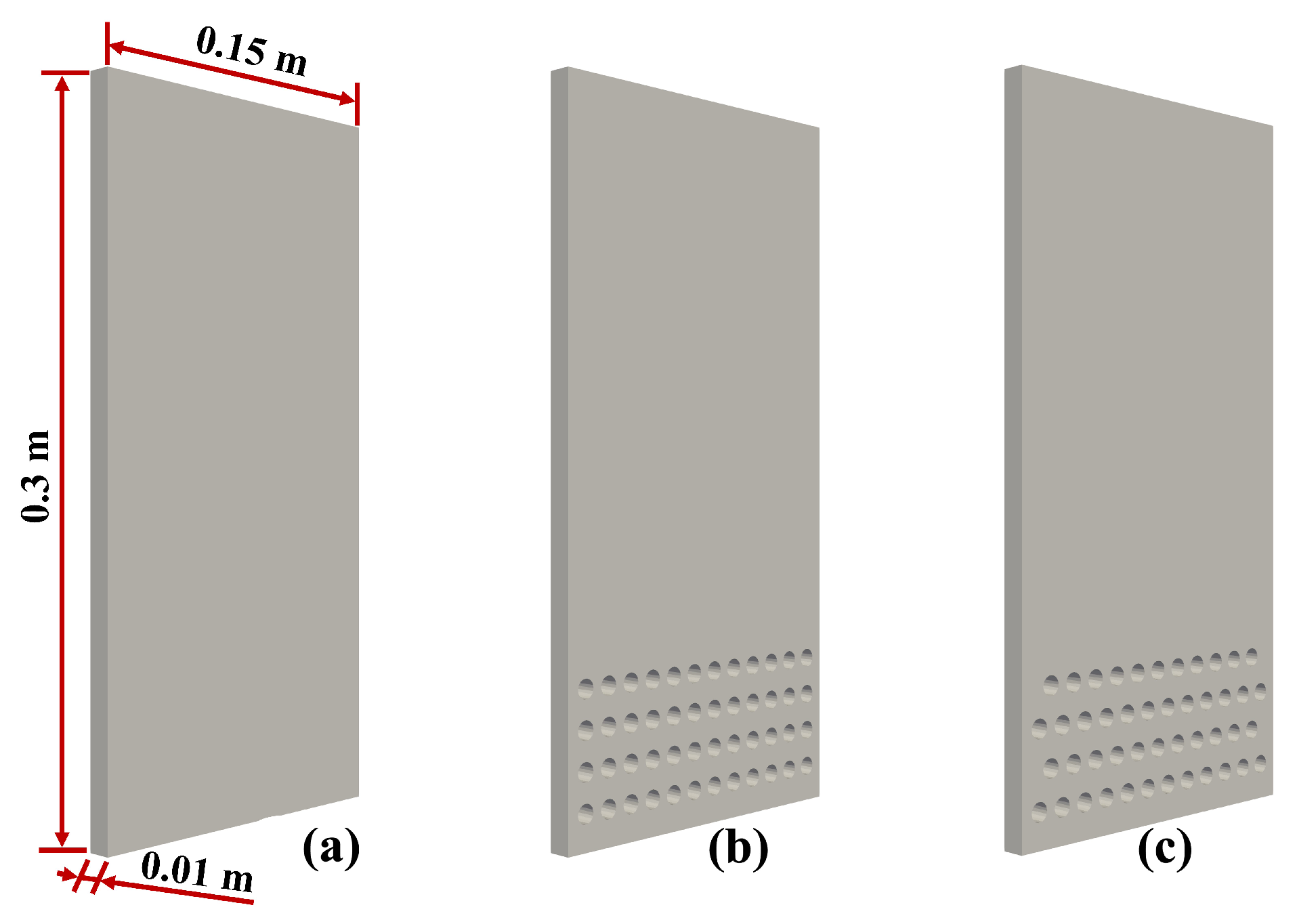
3. Setup of Simulation

The methanation reactors are shown in Figure 1. The height and width are 0.3 and 0.15 m, respectively. The depth of the reactor is 0.01 m. Reactor (a) is without cooling tubes. Reactor (b), with tubes, is the reference reactor in our work. The amount of cells is 165,300. Reactor (c), with staggered tubes, was used to investigate the influence of the arrangement. The amount of cells for reactor (c) is 165,108. The diameter of the immersed tube is 0.008 m. The horizontal distance between two tubes is 0.012 m. The vertical distance between two rows is 0.016 m. The mixture of CO and H${}_2$ was injected to the reactor from the bottom inlet, with the mole ratio 1:3. The gas inlet rate is 0.35 g/s for the reference case and N${}_2$ was used as the balance gas with 50% mass fraction. The catalyst is the Ni/Al${}_2$O${}_3$ particle with a density of 2000 kg/m${}^3$ and a diameter of 200 $\mathsf{\mu }$m. The total inventory is 87 g for all cases.

For the simulations, the $k-\epsilon$ model was adopted to model gas turbulence. The energy conservation equations were solved to obtain the temperature of the gas and solid phase. No-slip boundary conditions for the mean particle velocity was imposed. Outflow conditions were set for the outlet of the reactor with the atmosphere pressure. The code uses a cell-center type finite volume method with a second-order centered scheme in space and a first-order scheme in time. The semi-implicit fractional step method was adopted with iterative linear solvers.

4. Results and Discussion

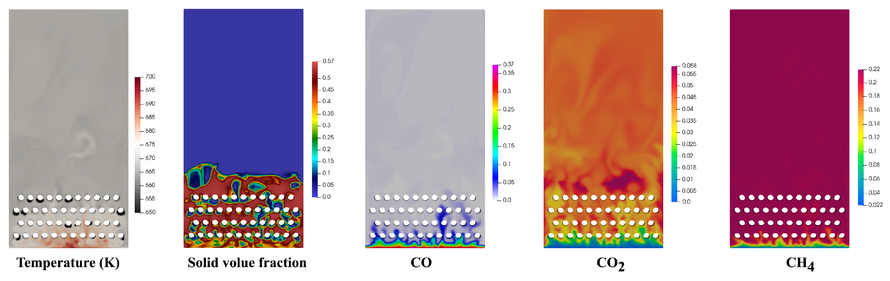
4.1. Performance of Reactor

The instantaneous distributions of gas components are shown in Figure 2. The nitrogen is used as a balance gas with 50% mass fraction. CO is almost completely converted in the region close to the inlet. H${}_2$ can be found at the outlet, which is the reactant of methanation, but also the product of the water–gas shift reaction. CH${}_4$ is produced simultaneously in the range of 1 centimeter from the inlet. The formation of CO${}_2$ lasts for a longer time and we can find the increase of the mass fraction of CO${}_2$ to the end of bed materials.

The time evolution of gas species mole fraction at the outlet is shown in Figure 3. At the initial time, the reactor is full of nitrogen. After 0.8 s, the products arrive at the outlet of the reactor. The heat removal is 1300 W for the reactor, which is decided after several simulations and theoretical predictions. The mole fraction at the outlet fluctuates around the constant value after 6 s, which illustrates that the system reaches the balance state under current conditions. The main component at the outlet is CH${}_4$ and H${}_2$O. The value of CO is quite low. A certain amount of carbon dioxide is detected at the outlet, which is the product of the water–gas shift reaction. The corresponding conversion rate is shown on the right of Figure 4. The conversion of CO and H${}_2$ are about 0.988 and 0.915, respectively. The lower conversion for H${}_2$ is caused by the production of H${}_2$ by the water–gas shift reaction. The selectivity of CH${}_4$ is 0.902, which indicates that most of the CO has been converted into CH${}_4$. Whilst, the selectivity of CO${}_2$ is about 0.098. Due to the occurrence of the water–gas shift reaction, some reactants are converted into CO${}_2$, which is hard to avoid when utilizing Ni as catalyst.

The most concerned and influential parameter in the current work is the temperature, as shown in Figure 5. The highest temperature occurs near the gas inlet. Because the methanation is a strong exothermic reaction, the temperature increases rapidly close to the inlet, with reaction heat released. With the gas and solid moving upward and encountering the tubes, the heat carried by gas and solid phases is removed by the cooling tubes and the temperature decreases. The time-evolution of temperature at the outlet is computed and shown in Figure 6. The temperature increases first and then reaches the nearly constant value after 6 s. Under the current conditions, the final temperature fluctuates around 683 K with heat removal 1300 W.

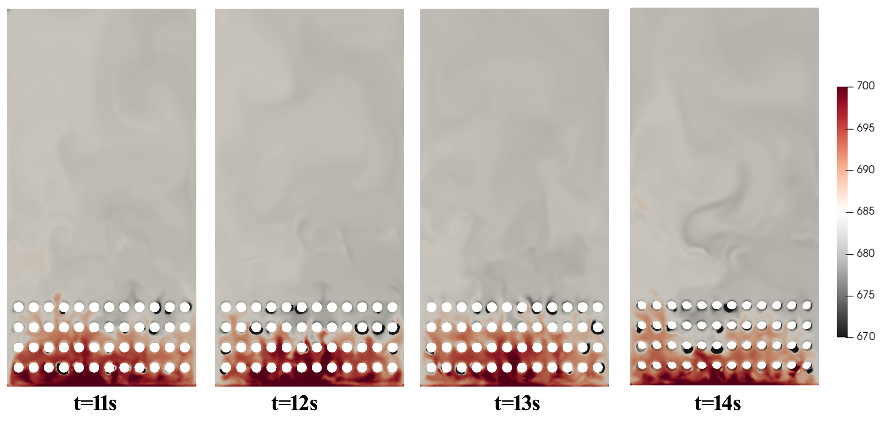
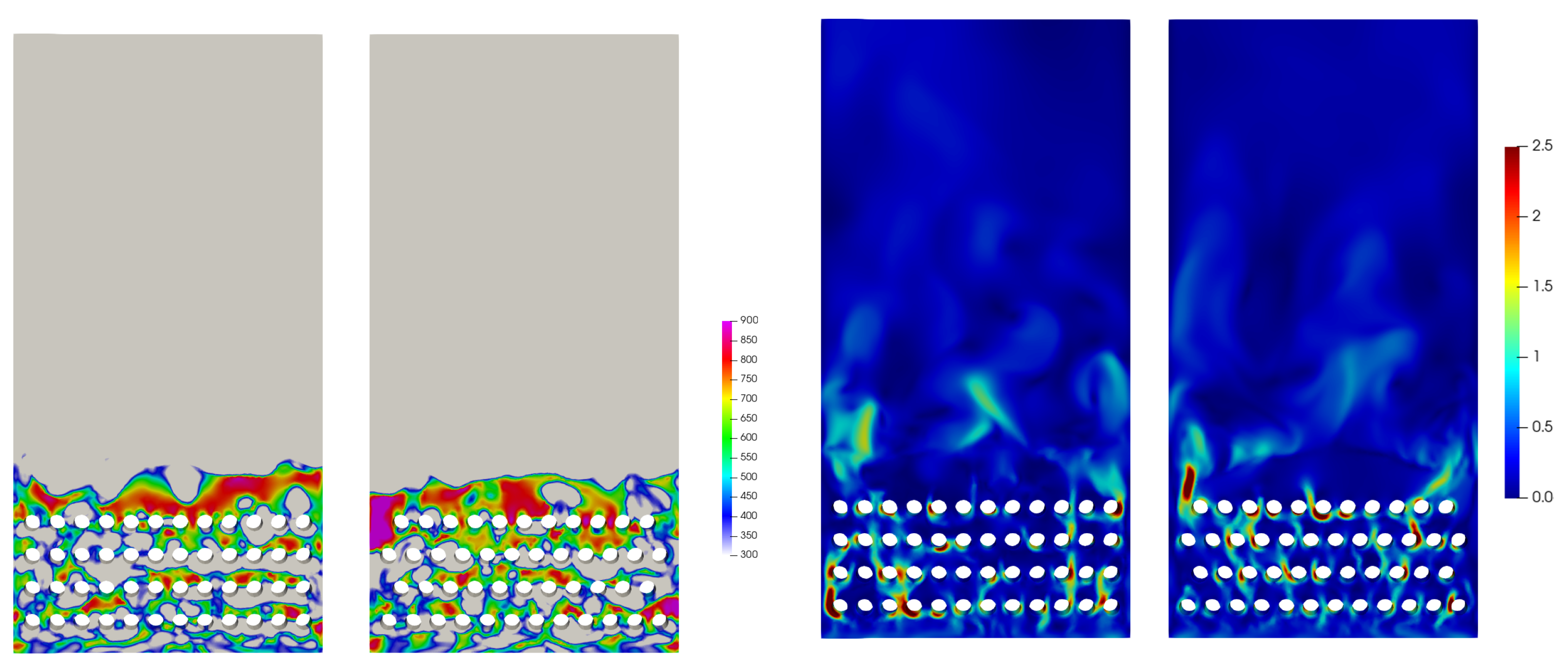
4.2. Influence of the Temperature

To investigate the influence of temperature on the performance of the methanation process, we carried out the cases with different cooling powers of the immersed tubes, 0 W, 1300 W, and 2000 W, which correspond to the temperature increase process, steady process, and temperature decrease process, to reveal the mechanism of the temperature on the methanation.

The profile of time-evolution gas temperature for different processes is shown in Figure 7. The dashed line represents the reference case with a steady state. With the current gas inlet rate, we found the heat removal of 1300 W was a suitable value for the current condition. For the case without heat removal, the temperature increased linearly to the end of the case. If we set the heat removal at 2000 W, the outlet temperature decreases. For these two dynamic cases, did not have the steady state at the end of the simulations. What we wanted to know was the influence of temperature during the changing process; each case was carried out for 25 s.

The conversion rates of CO and H${}_2$ are shown in Figure 8. The conversion rates of CO decrease with time for both cases. For the temperature increasing process (black line), the decline is smaller than that for the temperature decreasing process. The conversion rate of H${}_2$ is inversely proportional to the temperature. The same tendency can be found for the selectivity of CH${}_4$, as shown in Figure 9. When increasing the temperature, the selectivity of CO${}_2$ increases. It means that more reactants are converted into CO${}_2$ and we get less CH${}_4$ when we raise the operating temperature from steady state. Considering both the Figure 8 and Figure 9, we get that during the process of increasing the temperature, the water–gas shift reaction and reverse reaction were enhanced. The original chemical equilibrium was interrupted. By decreasing the temperature, more CH${}_4$ are generated and we get less CO${}_2$. The conversion of CO decreases due to the decreases of reaction kinetics. Until now, we know when the temperature is higher than the critical stability value, the chemical equilibrium is the dominant factor; when the temperature is lower than the critical stability value, the reaction is limited by the kinetics.

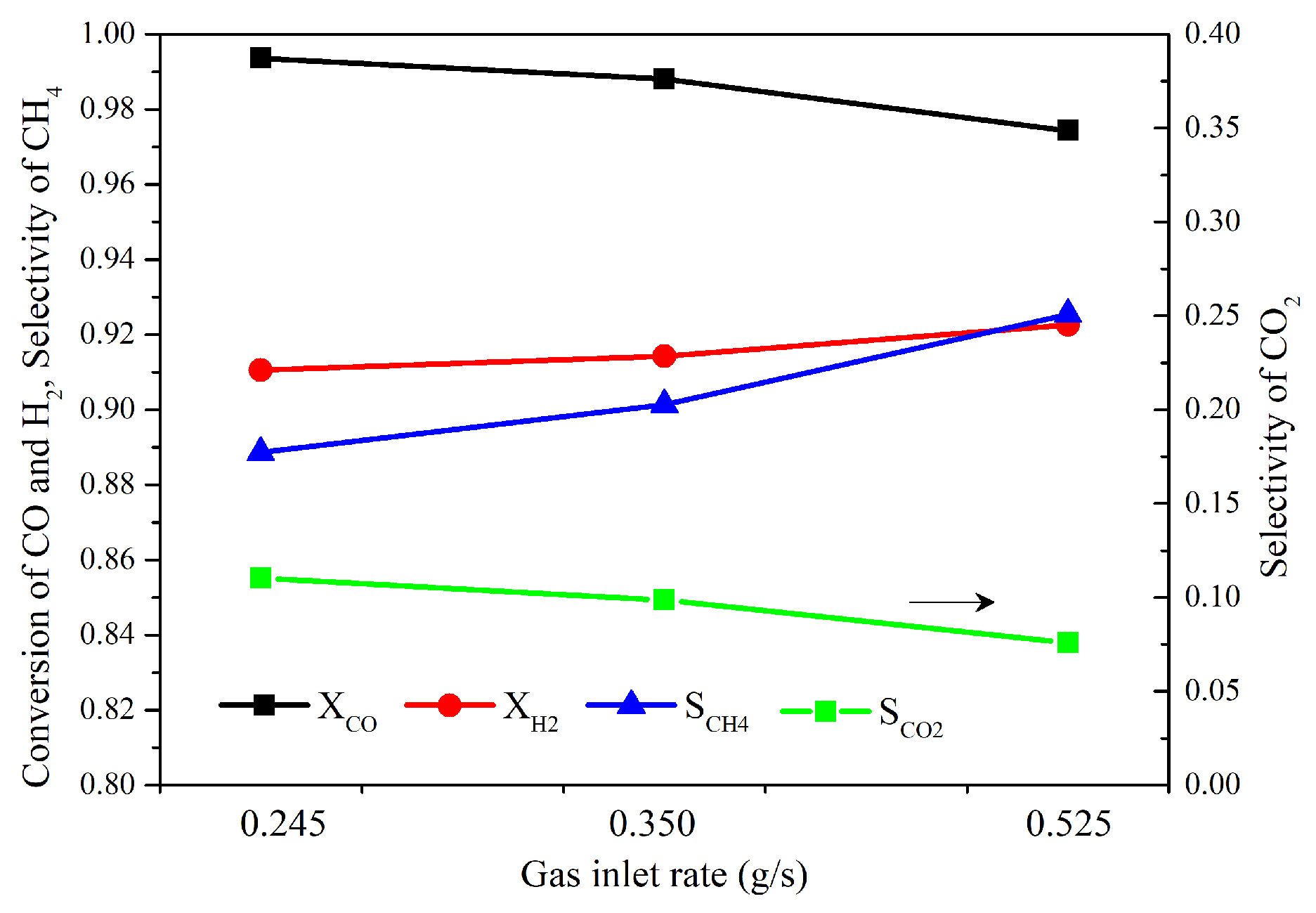
4.3. Influence of Flow Behavior

To investigate the influence of dynamic behavior, we tested the cases with different inlet rates. The flow rate of CO and H${}_2$ kept constant for all of the simulations to produce the same amount of reaction heat. The balance gas, N${}_2$, was adjusted to generate the different flow patterns and the flow rates of N${}_2$ are 0.070 g/s, 0.175 g/s and 0.345 g/s, respectively. The solid volume fraction is shown in Figure 10. The bed expanded height increases with the inlet rate. More (and larger) bubbles are formed around the tubes for the case with the higher gas inlet rate. The corresponding conversion rate of reactants and selectivity of products are shown in Figure 11. The CO conversion decreases with the inlet rate under the combining effect of residence time and the heat transfer. The conversion of H${}_2$ and selectivity of CH${}_4$ increase with the inlet rate. The selectivity of CO${}_2$ decreases with inlet rate.

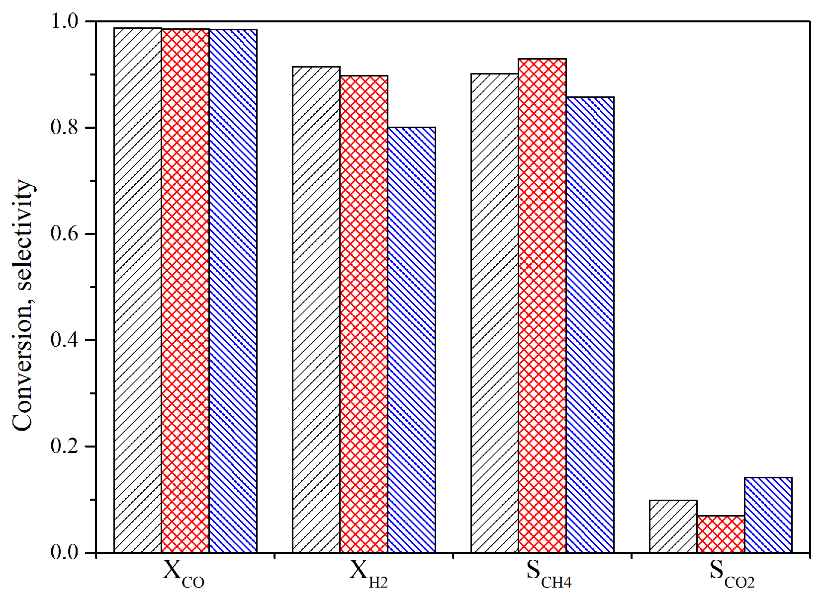
4.4. Influence of the Arrangement of Tubes

Three arrangements of immersed tubes are discussed in this section. The basic one is without tubes. The normal arrangement of tubes has been discussed in the first part of this section. The performance of the staggered tubes are shown in Figure 12. Compared with Figure 5, the temperature in the reactor with staggered tubes is lower than the reference case, which indicates the heat removal efficiency is higher with staggered tubes and the region with high temperature becomes narrow. The second sub-figure in Figure 12 shows the flow pattern with staggered tubes. CO${}_2$ is generated in the whole bed. We can find that methane is produced between the first and second row of tubes at the last sub-figure.

The Nusselt number is computed and shown in Figure 13. The highest value of $Nu$ for the staggered tubes case is larger than the reference case, which illustrates a larger heat transfer between the fluid and tubes. The gas velocity is shown on the right of Figure 13. For the case with staggered tubes, the gas detours between different rows of tubes. However, for the reference case, most gas will traverse the bed material without passing the channel between the rows. This leads to a lower performance of heat transfer for the reference case.

The conversion rate of reactants and selectivity of products for different plans of the reactors are shown in Figure 14 for quantitative analysis. The conversion rate of CO is quite high for all three cases. The case without tubes produces the least amount of CH${}_4$ and the largest of CO${}_2$ due to the reaction heat is not removed from the center of the reactor. Comparisons between the reference case and staggered arrangements of tubes show that the production of CH${}_4$ is larger with staggered tubes, and the lowest selectivity of CO${}_2$ was observed. The results indicate the optimal configuration should be the staggered one, which corresponds to the most effective removal of the reaction heat.

The interaction coefficient between phases are shown in Figure 15. The drag coefficient decreases with solid volume fraction. With the high solid volume fraction, the interaction between gas and solid is nearly the same for the case with normal arrangement and staggered arrangement. Difference between two configurations can be found at low solid volume fraction as shown on the right of Figure 15, the staggered tubes lead to a lower drag coefficient. The difference of the micro-dynamic behavior will finally generate the different performances of the reactor.

5. Conclusions

This numerical study was carried out to better understand the CO methanation process in a three-dimensional fluidized bed reactor utilizing a Euler–Euler two-fluid model. The performance of the methanation reactor and reaction characteristics were obtained and analyzed. The reaction heat removal was realized by the immersed tubes in the reactor. The influences of operating parameters on the production of methane were studied. Based on the current results, some essential issues can be explained, and the following conclusions can be drawn:

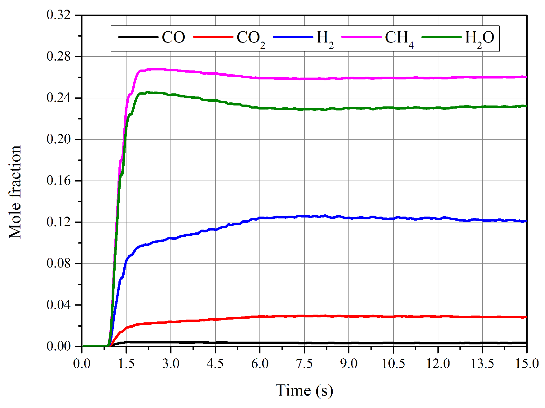
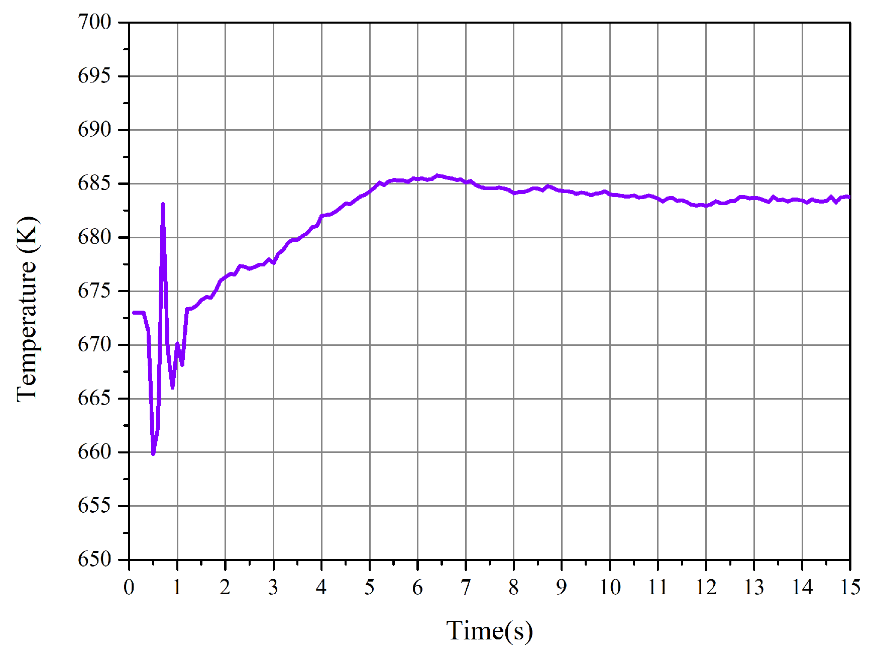
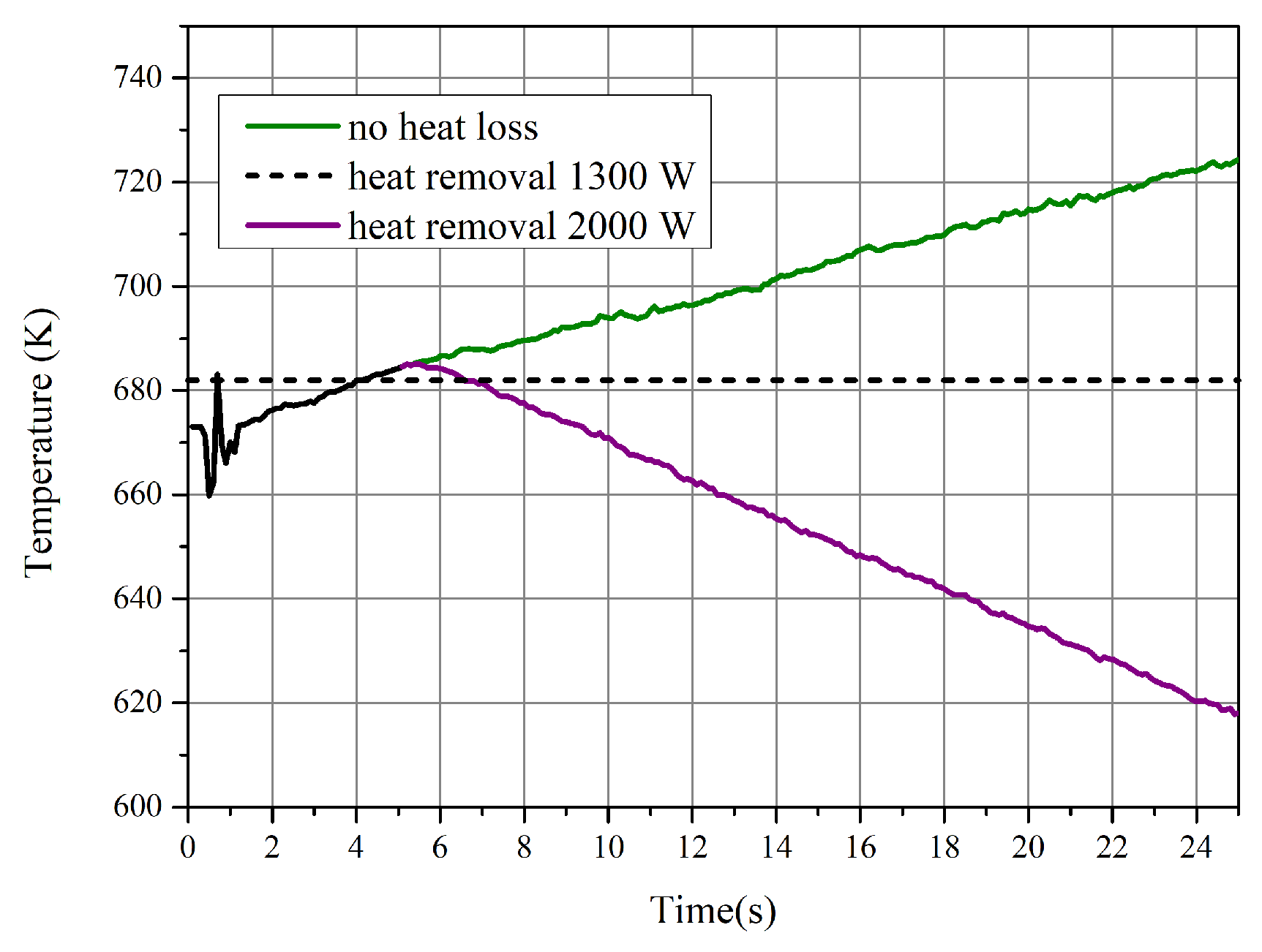
• The chemical equilibrium of the methanation process was achieved during the CFD simulation with effective heat removal by immersed pipes, and the preferable temperature was about 682 K. The results also show that the temperature has an essential impact on the production of methane.
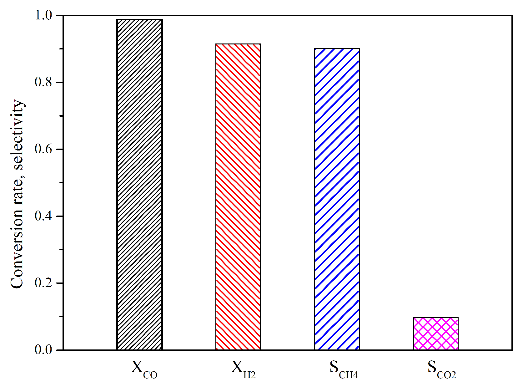
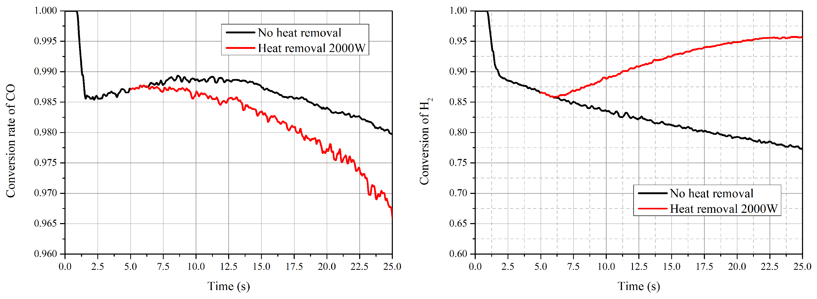
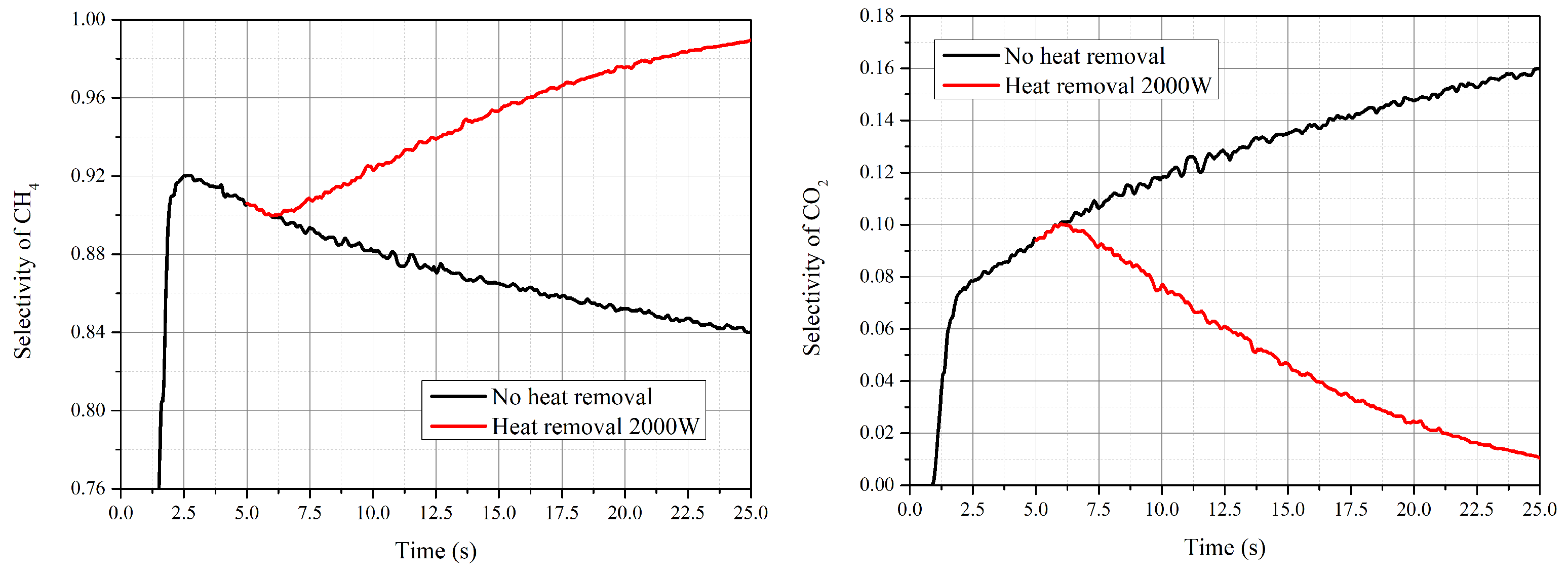
• The reaction finished near the inlet of the reactor, and then the main process was the mixing of the gas components. The CO vanished for each operating condition and the conversion rate was higher than 98%. The highest value of selectivity of methane was 92 % under current operating conditions.
• During the process of increasing temperature from the steady condition, the water–gas shift reaction and reverse reactions played a more important role for the performance of the reactor. The production rate of CH${}_4$ decreased and more reactants were converted into CO${}_2$. Chemical equilibrium was the decisive factor during the process with increasing temperature.
• With the decrease in temperature, the effect of the reaction kinetic became the dominant factor. The selectivity of CH${}_4$ increased, whilst the conversion rate of CO decreased due to the low reaction rate.
• The arrangement of the tubes will influence the interaction between the fluid and tubes. The staggered tubes are beneficial for the effective removal of reaction heat. The selectivity of methane with staggered tubes was 3% higher than that with normal tubes.
• The effect of the structures of the tubes, including the diameter, distance between tubes, and the amount of tubes, should be studied to determine the construction at the next stage.

References

1. Kopyscinski, J.; Schildhauer, T.J.; Biollaz, S.M.A. Employing Catalyst Fluidization to Enable Carbon Management in the Synthetic Natural Gas Production from Biomass. Chem. Eng. Technol. 2009, 32, 343–347. [Google Scholar] [CrossRef]
2. Hussain, I.; Jalil, A.; Hassan, N.; Farooq, M.; Mujtaba, M.; Hamid, M.; Sharif, H.; Nabgan, W.; Aziz, M.; Owgi, A. Contemporary thrust and emerging prospects of catalytic systems for substitute natural gas production by CO methanation. Fuel 2021, 122604. [Google Scholar] [CrossRef]
3. Gao, J.; Liu, Q.; Gu, F.; Liu, B.; Zhong, Z.; Su, F. Recent advances in methanation catalysts for the production of synthetic natural gas. RSC Adv. 2015, 5, 22759–22776. [Google Scholar] [CrossRef]
4. Liu, P.; Zhao, B.; Li, S.; Shi, H.; Ma, M.; Lu, J.; Yang, F.; Deng, X.; Jia, X.; Ma, X.; et al. Influence of the Microstructure of Ni–Co Bimetallic Catalyst on CO Methanation. Ind. Eng. Chem. Res. 2020, 59, 1845–1854. [Google Scholar] [CrossRef]
5. Rönsch, S.; Schneider, J.; Matthischke, S.; Schlüter, M.; Götz, M.; Lefebvre, J.; Prabhakaran, P.; Bajohr, S. Review on methanation – From fundamentals to current projects. Fuel 2016, 166, 276–296. [Google Scholar] [CrossRef]
6. Kopyscinski, J.; Schildhauer, T.J.; Biollaz, S.M. Methanation in a fluidized bed reactor with high initial CO partial pressure: Part II— Modeling and sensitivity study. Chem. Eng. Sci. 2011, 66, 1612–1621. [Google Scholar] [CrossRef]
7. Eri, Q.; Peng, J.; Zhao, X. CFD simulation of biomass steam gasification in a fluidized bed based on a multi-composition multi-step kinetic model. Appl. Therm. Eng. 2018, 129, 1358–1368. [Google Scholar] [CrossRef]
8. Kopyscinski, J.; Schildhauer, T.J.; Biollaz, S.M. Methanation in a fluidized bed reactor with high initial CO partial pressure: Part I—Experimental investigation of hydrodynamics, mass transfer effects, and carbon deposition. Chem. Eng. Sci. 2011, 66, 924–934. [Google Scholar] [CrossRef]
9. Kopyscinski, J.; Schildhauer, T.J.; Biollaz, S.M.A. Fluidized-Bed Methanation: Interaction between Kinetics and Mass Transfer. Ind. Eng. Chem. Res. 2011, 50, 2781–2790. [Google Scholar] [CrossRef]
10. Cobb, J.T.; Streeter, R.C. Evaluation of Fluidized-Bed Methanation Catalysts and Reactor Modeling. Ind. Eng. Chem. Process Des. Dev. 1979, 18, 672–679. [Google Scholar] [CrossRef]
11. Yu, H.; Zhang, H.; Buahom, P.; Liu, J.; Xia, X.; Park, C.B. Prediction of thermal conductivity of micro/nano porous dielectric materials: Theoretical model and impact factors. Energy 2021, 233, 121140. [Google Scholar] [CrossRef]
12. Li, J.; Yang, B. Multi-scale CFD simulations of bubbling fluidized bed methanation process. Chem. Eng. J. 2019, 377, 119818. [Google Scholar] [CrossRef]
13. Chein, R.Y.; Yu, C.T.; Wang, C.C. Numerical simulation on the effect of operating conditions and syngas compositions for synthetic natural gas production via methanation reaction. Fuel 2016, 185, 394–409. [Google Scholar] [CrossRef]
14. Liu, Y.; Hinrichsen, O. CFD Simulation of Hydrodynamics and Methanation Reactions in a Fluidized-Bed Reactor for the Production of Synthetic Natural Gas. Ind. Eng. Chem. Res. 2014, 53, 9348–9356. [Google Scholar] [CrossRef]
15. Li, J.; Yang, B. Bubbling fluidized bed methanation study with resolving the mesoscale structure effects. AIChE J. 2019, 65, 16561. [Google Scholar] [CrossRef]
16. Ich Ngo, S.; Lim, Y.I.; Lee, D.; Won Seo, M.; Kim, S. Experiment and numerical analysis of catalytic CO2 methanation in bubbling fluidized bed reactor. Energy Convers. Manag. 2021, 233, 113863. [Google Scholar] [CrossRef]
17. Zhang, W.; Machida, H.; Takano, H.; Izumiya, K.; Norinaga, K. Computational fluid dynamics simulation of CO2 methanation in a shell-and-tube reactor with multi-region conjugate heat transfer. Chem. Eng. Sci. 2020, 211, 115276–115285. [Google Scholar] [CrossRef]
18. Li, J.; Agarwal, R.K.; Yang, B. Two-Dimensional Computational Fluid Dynamics Simulation of Heat Removal in Fluidized Bed Methanation Reactors from Coke Oven Gas Using Immersed Horizontal Tubes. Ind. Eng. Chem. Res. 2020, 59, 981–991. [Google Scholar] [CrossRef]
19. Zhang, Q.; Cao, Z.; Ye, S.; Sha, Y.; Chen, B.; Zhou, H. Mathematical modeling for bubbling fluidized bed CO-methanation reactor incorporating the effect of circulation and particle flows. Chem. Eng. Sci. 2022, 249, 117305. [Google Scholar] [CrossRef]
20. Sun, L.; Luo, K.; Fan, J. 3D Unsteady Simulation of a Scale-Up Methanation Reactor with Interconnected Cooling Unit. Energies 2021, 14, 7095. [Google Scholar] [CrossRef]
Figure 1. Structure of the fluidized bed methanation reactor. (a) without tubes, (b) with normal arranged tubes, (c) with staggered tubes.
Energies 15 00321 g001
Figure 2. Snapshot of instantaneous mass fraction of gas species. Nitrogen is utilized as balance gas.
Energies 15 00321 g002
Figure 3. Profile of the time-evolution of the gas species mole fraction at the outlet of the reactor.
Energies 15 00321 g003
Figure 4. Profile of the time-averaged conversion rate of the reactants and the selectivity of products.
Energies 15 00321 g004
Figure 5. Distribution of instantaneous temperatures at different time points.
Energies 15 00321 g005
Figure 6. Time-evolution of temperature at the outlet of the methanation reactor.
Energies 15 00321 g006
Figure 7. Profile of the time-evolution gas temperature. Dashed line: reference case with heat removal, 1300 W. Green line: no heat removal. Purple line: heat removal 2000 W.
Energies 15 00321 g007
Figure 8. Time-evolution of conversion rate of CO (left) and H 2 (right).
Energies 15 00321 g008
Figure 9. Time-evolution of selectivity of CH 4 (left) and CO 2 (right).
Energies 15 00321 g009
Figure 10. Profile of the solid volume fraction with different fluidization gas inlet rate; (a) 0.245 g/s, (b) 0.35 g/s, (c) 0.525 g/s.
Energies 15 00321 g010
Figure 11. Conversion rate of reactants and selectivity of products with different fluidization gas rates.
Energies 15 00321 g011
Figure 12. Instantaneous distribution of temperature, solid volume fraction, mass fraction of CO, CO 2 , and CH 4 .
Energies 15 00321 g012
Figure 13. (Left): instantaneous distribution of the Nusselt number. (Right): instantaneous distribution of gas velocity.
Energies 15 00321 g013
Figure 14. Conversion rate and selectivity under different configuration. Black column: normal arrangement of tubes. Red column: staggered arrangement of tubes. Blue column: without tubes.
Energies 15 00321 g014
Figure 15. (Left): distribution of the drag coefficients for the case with staggered tubes. (Right): fitting results of the drag coefficient for different arrangement of tubes.
Energies 15 00321 g015