Uncovering Contributing Factors to Interruptions in the Power Grid: An Arctic Case

Abstract

Electric failures are a problem for customers and grid operators. Identifying causes and localizing the source of failures in the grid is critical. Here, we focus on a specific power grid in the Arctic region of Northern Norway. First, we collected data pertaining to the grid topology, the topography of the area, the historical meteorological data, and the historical energy consumption/production data. Then, we exploited statistical and machine-learning techniques to predict the occurrence of failures. The classification models achieve good performance, meaning that there is a significant relationship between the collected variables and fault occurrence. Thus, we interpreted the variables that mostly explain the classification results to be the main driving factors of power interruption. Wind speed of gust and local industry activity are found to be the main controlling parameters in explaining the power failure occurrences. The result could provide important information to the distribution system operator for implementing strategies to prevent and mitigate incoming failures.

1. Introduction

Failures in electricity supply from producers to customers affect anyone connected to the distribution grid [1,2,3,4]. In the case of the distribution system operator (DSO), power interruptions are considered as a breach of the contractual obligations with the consumers and result in financial penalties [5].

Electric failures alone can turn into serious losses whose estimates range from $22 to $135 billion annually [6,7,8]. Moreover, failures might have complex and adverse socio-economic consequences in communities heavily reliant on the electricity supply [9,10].

This study focuses on a specific grid in the Arctic region of North Norway. In this context, the expansion of local industries connected to the power grid is driven by the processing and exporting of fish to the worldwide market. An important requirement is that these production lines operate at full capacity during the high season. These industries adopt several automated components that are critically dependent on reliable power quality. Even minor electrical disturbances lasting only a few seconds could stop the entire production line for a significant amount of time. In particular, for every short-term power interruption that occurs, 40 min to 1 h might pass before resuming production.

In most communities, multiple sources could provide backup electricity supply if one line is interrupted [11]. However, the power grid considered in our study has a radial distribution system where customers connected to the grid do not have any sources to provide backup power in case of a failure. Therefore, it is fundamentally important to increase the reliability of the power grid.

One way to deal with this situation is to build a new power grid and design it to handle the current power requirements.

However, building a new power grid has an enormous environmental impact, requires large investment costs, and is a time-consuming process. Moreover, this does not fit in with the vision of making better use of today’s power grid [12,13]. In addition, if the industries that are currently connected to the grid will stop their activities, the power company will end up with an over-dimensioned power grid. Rather than investing in a new power grid, it is possible to reduce the number of failures in the current power grid. However, this implies that the factors that cause the power failures must be identified.

The identification of such factors, and their location in the grid, has proven to be a major challenge for the DSO [14].

So far, the DSO has accepted the numerous failures in the power grid and has operated the grid in the best possible way given the failures that occur. However, new regulations have made it more expensive for the DSO to tolerate failures in the power distribution network and, at the same time, the more automated industries have much higher requirements for high power quality than before.

Therefore, there is a huge motivation for the DSO to identify in detail the factors triggering power interruptions to be able to operate the grid in a better way.

The increased availability of energy-related data by the DSOs makes it now possible to exploit data science techniques to develop strategies to improve the reliability of the power grid [15]. Some effort has been put in this direction where the performance of the proposed solutions has been applied on benchmark power systems [16,17]. Results indicate that extreme weather conditions are often the major cause of failures in the power grid. Indeed, resent research investigate the relationships between weather variables and power failures with the use of machine learning (ML) [6]. However, it is likely that besides weather conditions, human activity also plays a key role.

In this work, in close collaboration with the DSO, we construct a dataset considering a wider spectrum of explanatory variables that could explain the onset of a power failure. In particular, rather than assuming that harsh weather conditions are the only source of failures, we also consider measurements of electricity-related variables. Once the dataset is constructed, we exploit ML classification techniques to find the relationship between the failure and non-failure (i.e., normal condition) classes. In the end, we discover the variables that contribute the most to the power failure occurrence by interpreting the decision process of the ML classifiers.

The work is structured as follows. In Section 2, we review relevant related work. In Section 3, the specific power grid analyzed here is presented together with the report of failures from the local DSO. In Section 4, we present the methodology for building the dataset used in the statistical analysis. In Section 5, the different ML techniques used for classification and failure detection are presented. In Section 6, the features are analyzed, and we investigate the quality of the models in relation to the identification of the cause of failures. Conclusions are given in Section 7.

2. Related Works

2.1. Detecting Failures Caused by Weather Conditions

While prior studies on this topic are limited, harsh weather conditions are believed to be an important source of failures, and several studies have been conducted to address the impact of weather events on power quality.

A power system with high power quality is characterized by few power interruptions, a steady voltage, a steady frequency (close to 50 Hz in Europe), and a smooth sinusoidal voltage curve.

In the study by Owerko et al., power failures in New York City were predicted based on weather conditions [6]. The authors deployed a Graph Neural Network (GNN) to adequately process weather measurements close to the power grid to determine the likelihood of power failure. The results showed a 1.04% error in the prediction.

Perera et al. analyzed the impact of extreme weather events on the reliability of power systems in 30 cities in Sweden [18]. The authors developed an optimization method to consider both extreme and less extreme weather events, and the results indicated that in periods with extreme weather, the power supply reliability dropped by 16%.

The authors in [17] provide a framework for quantifying and modeling the resilience of power systems that addresses the challenge of high wind incidences. In this work, they accounted for all possible routes from power generators to loads by proposing a matrix-based approach. Here, the load importance before and after a failure event was considered. The effectiveness of the approach was tested on the IEEE 14-Bus system.

In the work by Trakas et al., the impact of frequent extreme weather events on the power grid supply reliability was addressed [16]. Here, a spatial risk analysis methodology was proposed. This analysis tool could provide a warning when there is an evolving risk for failure for a system placed in regions that is more exposed to extreme weather events. In addition, a Severity Risk Index (SRI) was used to monitor the power system in real time. The SRI considered both the spatial and temporal evolution of the extreme event, the system performance, and the system operating conditions during the extreme weather event.

Reference [19] reviews existing methodologies where they assess the impact of weather on power system resilience. Critical infrastructure and plans for improving resilience in cases of extreme weather events are also provided.

The authors in [20] together with the Italian Transmission System Operator (TSO) proposed an approach to improve grid resilience in natural disastrous events. The approach deploys flexibility tools that combine the flexibility margins of the networks to those of generation and load. The authors propose a flexibility tool to improve the resilience of the power system in case of severe weather conditions.

Common for all studies that have been presented here is that most studies test their proposed approach on benchmark datasets rather than on real-world problems. In addition, the studies only consider severe weather events and disregard factors such as failures caused by human activities.

2.2. Alternative Approaches for Failure Detection

In Hoffmann et al. [21], a methodology to predict incoming power failures was proposed. In this work, the authors analyzed high-resolution data from Power Quality Analyzers (PQAs) and Phasor Measurement Units (PMUs). The main aim of the work was to predict power interruptions, voltage drops, and earth failures by analyzing measurements from nine real-world PQA nodes in the Norwegian power grid. In conclusion, the authors reported that the incipient power interruptions were easiest to predict, while voltage dips and earth failures were more challenging to predict.

The long-lasting challenge for the DSO of detecting earth failures has been recently addressed [22], which shows that by integrating advanced metering infrastructure with a distribution management system, failures can be detected. However, the proposed solution can only be used if the DSOs have access and know how to use the OpenDSS software.

The challenge of the increasing strain on the power grid with increasing electrification has also been investigated [23]. Here, the challenge with the implementation of renewable energy technologies with intermittent power production is discussed. The authors proposed possible monitoring solutions and failure-predicting methodologies by using statistics and field measurements from the Norwegian power grid. While ML approaches were identified as candidates, the authors did not use any. No time resolution and/or duration was considered either in terms of developing a robust failure detection and prediction methodology.

In this section, relevant works on predicting power failures have been reviewed. All the former works have either only considered power-related measures or weather variables. The goal of this work is to consider both weather variables and power-related measures at the same time to provide a better overview of the potential variables that could result in power failures.

Here, the DSO that operates the grid that is analyzed has provided insight about the potentially relevant variables that could explain power failures.

In addition, none of the former work has proposed a technique to interpret the decision process of the machine learning (ML) models, which allows identifying the main important features that cause failures in the power grid.

3. Case Study

3.1. The SVAN22LY1 Power Grid

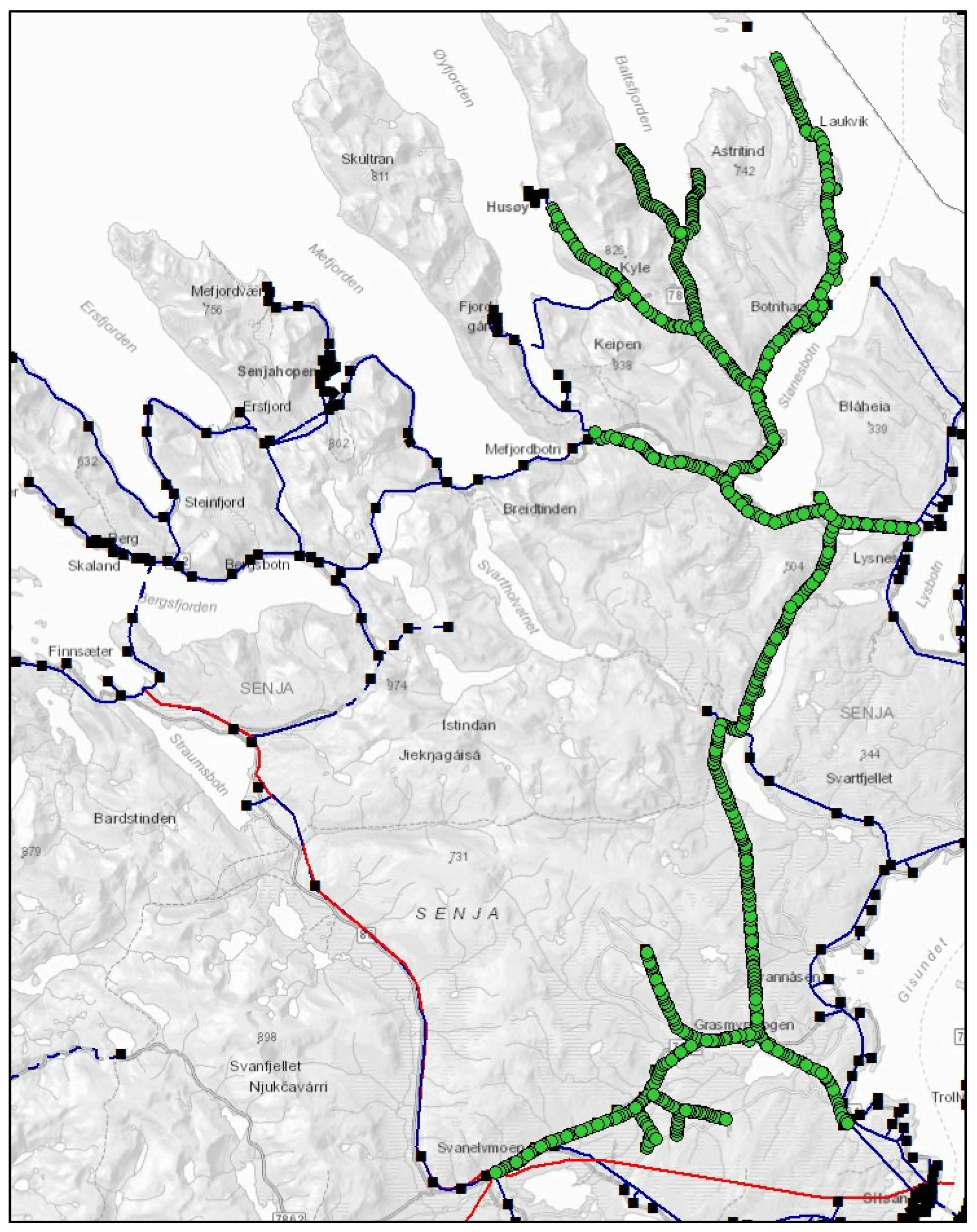
The power grid analyzed is a distribution system with a radial design, where the power flows from the south toward the north. The DSO of this power grid is the Arva Power Company, which has named this specific grid that is analyzed as SVAN22LY1. Figure 1 shows the whole power grid indicated by green dots.

The power line of the SVAN22LY1 power grid is supported by 978 utility poles with different geographical positions. The power grid spans 60 km from south to north. In Figure 1, the black boxes are the electrical transformers, while the red lines are the power grid with an operating voltage of 66 kilo Volt (kV). The blue lines and the SVAN22LY1 power grid covered in green dots have an operating voltage of 22 kV [14].

The largest customers connected to the SVAN22LY1 grid are located at the end of the northernmost point of the radial (69.546° N, 17.657° E). The total energy demand in the community is a combination of load profiles from two sectors: households and industry. Being a rural community, the industry accounts for more than 50% of the total energy consumption [24]. The industry has electrical machines that are sensitive to stable power quality, and minor power interruptions could bring the production line to a halt.

The SVAN22LY1 grid has one electrical transformer in the southern part of the grid (referred to as “Transformer south” in the following). This electrical transformer station provides information about the energy consumption for all customers connected to it and also for customers that are not directly connected to the SVAN22LY1 grid. Therefore, this electrical transformation station could provide insight into whether other types of energy consumption patterns than the local industry could affect the power quality.

There is a hydropower station connected directly to the SVAN22LY grid that generates electricity to support the grid. This hydropower plant is important to consider when analyzing the power supply reliability for SVAN22LY1. For instance, in periods when the hydropower plant operates at low capacity (or is shut down), electricity must be imported from other supply sources farther away from the power grid. This will result in feeder losses, i.e., losses of energy when being transported on the power line. The longer the distance of a power line, the larger the feeder losses. Therefore, if the local hydropower station does not generate electricity, the feeder losses would create voltage drop and have a negative impact on the local power quality.

In addition, if electricity must be imported from other sources, neighboring parts of the power grid could be overloaded and in the worst case result in failure [25]. The location of the key devices connected to the grid is described in Section 4.1.

In addition to the different consumption and production devices that could affect the power quality, the SVAN22LY1 power grid is in an area characterized by typical Arctic conditions with cold, long winters and is heavily exposed to harsh weather throughout the whole year. Harsh weather can cause voltage drops and power interruption, in addition to the increased power demand from end customers. For example, strong wind gusts can make the power lines between the utility poles collide, which can cause short-term (up to 1 min) interruptions in the power supply [26].

3.2. Reported Failures in the SVAN22LY1 Power Grid

Every failure in the power system is logged as an incident in the Norwegian reporting system FASIT (Failure-and interruption statistics within the national power grid) [27]. Each DSO company in Norway is required to have a FASIT reporting system. The purpose of FASIT is to provide information about the delivery reliability of the Norwegian power system. The report provides both information about historical delivery reliability and information for estimating future expected delivery reliability. To be able to obtain information on the delivery reliability, the report should contain information on:

• Operational disturbances;
• Planned disconnections that have led to power interruptions (both planned notified disconnection and planned unannounced disconnection).

The operational disturbances should cover information about each failure, on which grid the failure occurs and, if known, the reason for the failure. The operational disturbances should also cover an end-user focus by reporting the duration of the interrupted power. In addition, the amount of not-delivered power and the compensation for not-delivered power are reported [27]. The FASIT system also holds information about short-term power interruptions that typically are less than one minute.

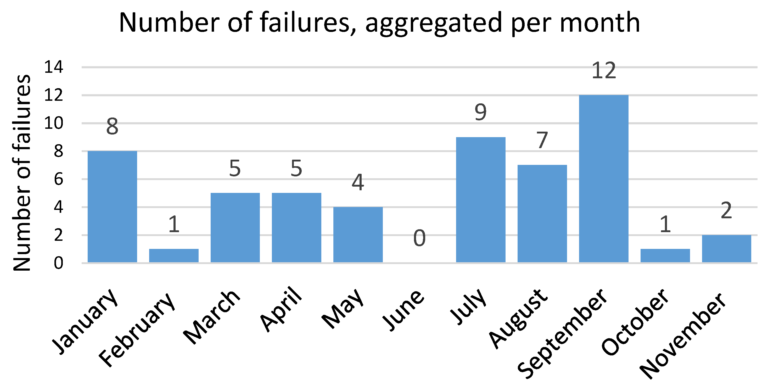
In this study, the FASIT report for the SVAN22LY1 grid is provided by the Arva Power Company [14]. In 2020 (January to the end of November), the FASIT system reported 54 incidents distributed over 44 different hours (several failures can occur within one hour). Figure 2 shows the reported failures in 2020. The distribution of failures during the year is not uniform, and most failures were reported in September month followed by January and July. In June, no failures were reported. Despite there being higher energy consumption from customers and more harsh weather conditions in the winter, there are more failures during the summer. The reason is that the local hydropower plant connected to the grid (more information about this hydropower plant in Section 4.1.3) operates with a reduced capacity compared to the rest of the year and, from time to time, it is completely shut down. This allows saving water, which can be used in winter when there is a larger need for electricity. This makes the power grid more vulnerable during the summer and exposed to power faults caused by a sudden demand for power from the industrial customers connected to the grid.

In this study, the period from the first of January 2020 to the end of November 2020 is investigated.

Since the FASIT only reports that a fault occurred somewhere in the grid, it is challenging to identify what caused the fault and on which part of the grid the fault occurred.

4. Method

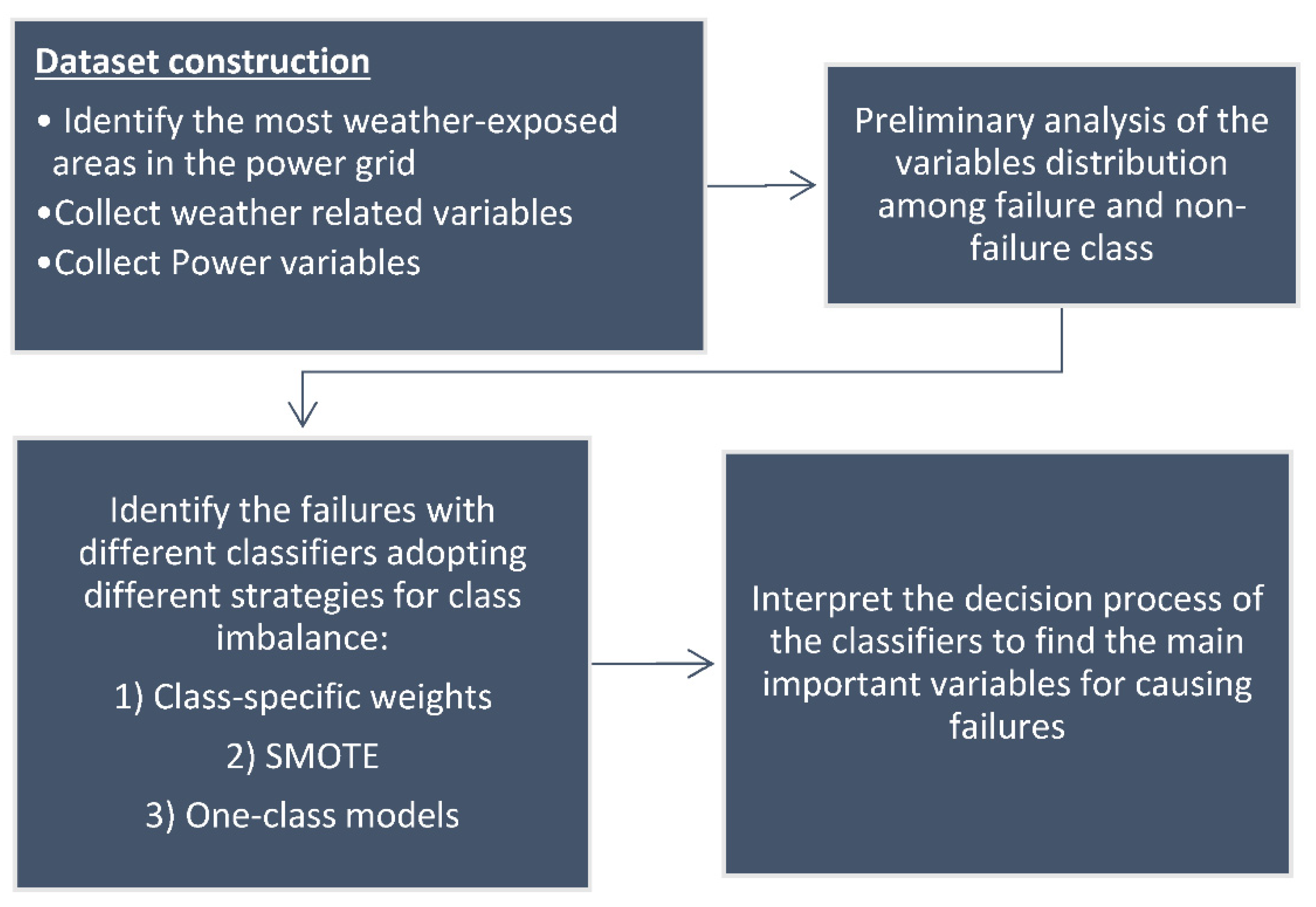
In Figure 3, a flow chart of the methodology is provided. The flow chart provides an overview of the different steps from first obtaining the dataset that is used to detect the failures with machine learning techniques to the final step where the main important variables for causing failures are identified.

4.1. Construction of the Dataset

To detect the potential contributing factors for failures, all potential variables of interest are collected. The candidate variables are divided into two groups: weather-related failures and energy-related (consumption-and production) failures.

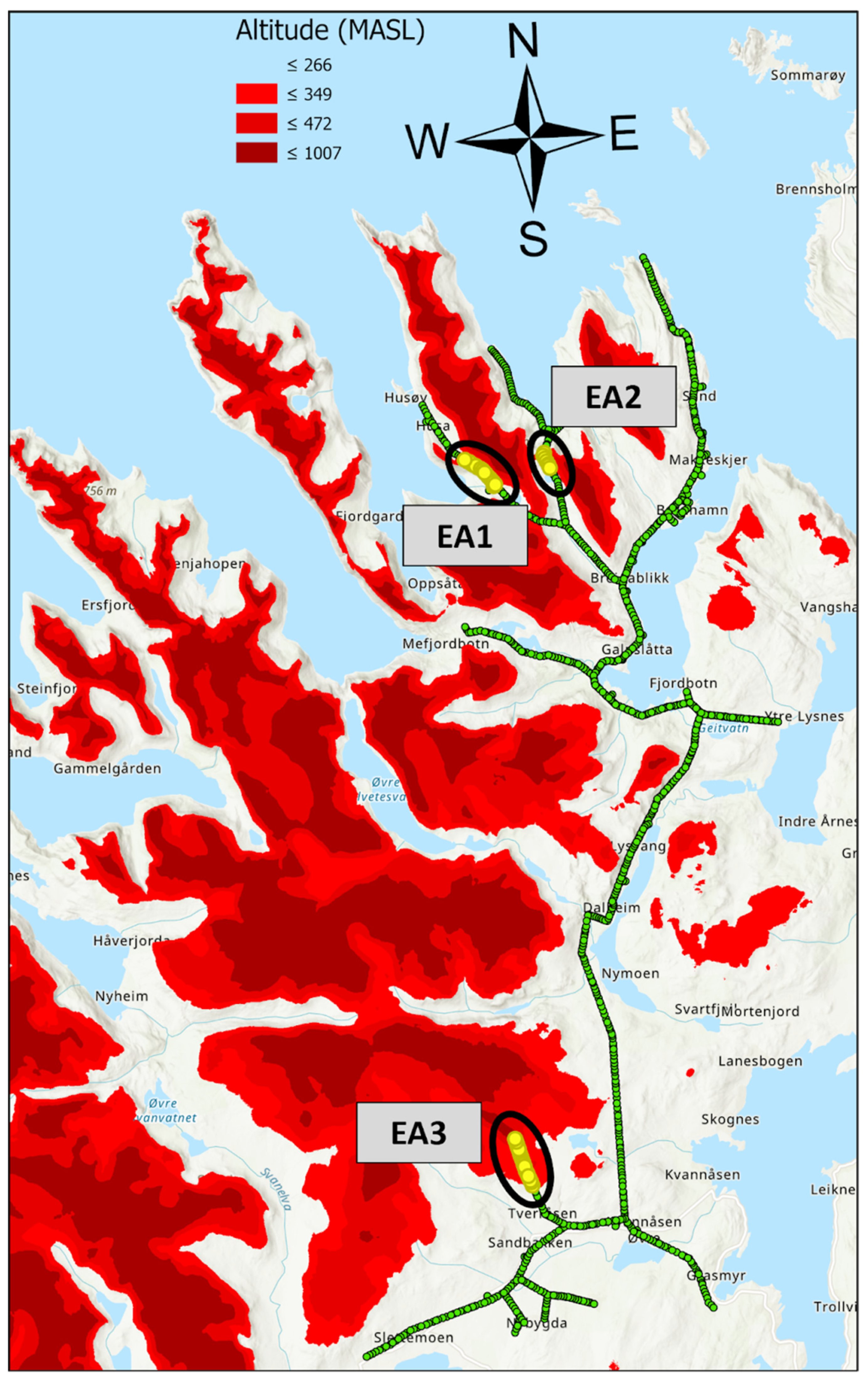
4.1.1. Localizing Weather-Exposed Areas in SVAN22LY1

As the SVAN22LY1 grid spans over a large area, the weather conditions can change significantly in different parts of the grid. To detect the regions that are more likely exposed to weather-related failures, some assumptions are required. One is to assume that higher elevation increases the probability of being exposed to harsh weather conditions, such as strong wind. Indeed, utility poles at high altitudes are often in mountainous areas where there is no vegetation that can protect from the wind.

The altitude map for the area of interest is obtained from the Norwegian Mapping Authority [28]. The altitude of each pole is obtained by checking its coordinates on a digital surface model (DSM) with a spatial resolution of 1 m [28,29]. The poles at the lowest altitude are at sea level (0 MASL (Meters Above Sea Level)), whereas the utility pole at the largest elevation is at 485 MASL. We group the altitudes into 5 groups: 1 (0–100 MASL), 2 (100–200 MASL), 3 (200–300 MASL), 4 (300–400 MASL), and 5 (400–485 MASL). We assume that the most exposed areas (EA) belong to group 4 and 5 (300 to 485 MASL).

The second information that is useful to consider is the distance between the utility poles. We assume that the longer the length between two poles, the higher the likelihood that the cables will collide under harsh weather conditions, resulting in power interruptions. The distance between adjacent utility poles is found by calculating the geodesic distance between the Lat–Long coordinates of each utility pole.

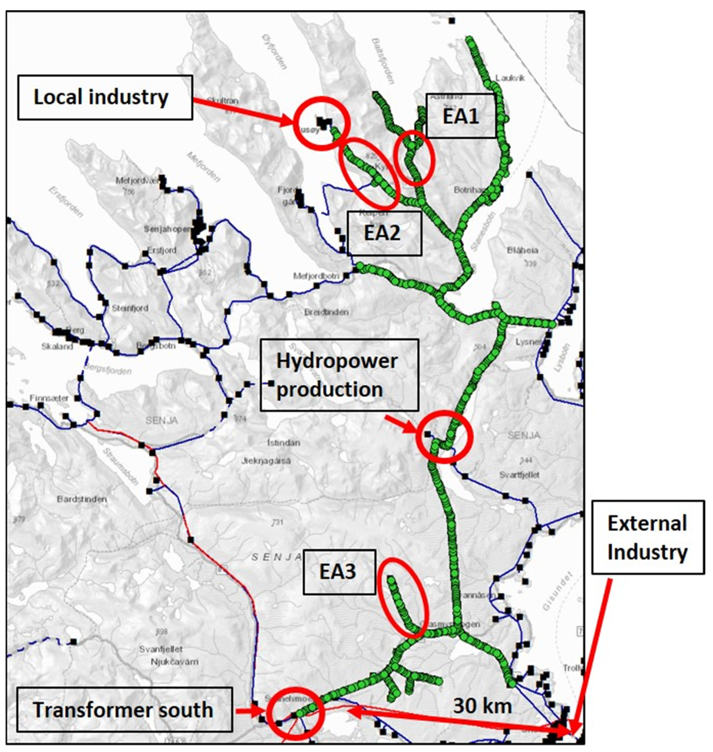
Based on the altitude and distances between poles, we selected 3 exposed areas (EAs). While there is no guarantee that these are the only areas that might trigger weather-related failures, this allows us to significantly narrow down the candidate regions. The utility poles in EAs are highlighted in Figure 4, and additional details are given in

Table 1. Properties of selected weather-exposed areas in the SVAN22LY1 power grid.

	EA1	EA2	EA3
Coordinate (deg.)	69.523 N, 17.779 E	69.520 N, 17.726 E	69.321 N, 17.729 E
Elevation (MASL)	300	360	485
Longest distance between poles (m)	122	136	121

.

4.1.2. Exposed Areas and Weather Variables from AROME-Arctic

The selected EAs are located kilometers apart (see Figure 3), and there is no weather station located in the proximity of each region. Therefore, to collect relevant weather data in the specific regions, we use the AROME-Arctic weather model developed by the metrological institute of Norway (MET). This is a reanalysis model that has run since November 2015 and has a spatial resolution of 2.5 km. AROME-Arctic accounts for weather conditions that are unique in Arctic regions, such as polar lows and icin [30]. The model covers the latitudes from 66 N to 88 N and longitudes from −18 E to 80 E.

From AROME-Arctic, the following variables in the EAs were collected: wind direction, wind strength, precipitation, relative humidity, temperature, and pressure. The variables were chosen based on the experiences from the DSO and the local customers, which reported the failures to be more likely in the presence of certain weather conditions. In particular, the weather variables were collected due to the following reason:

-

Wind speed of gust and wind direction were selected as relevant variables as they could cause collisions of the power lines. A collision of power lines will result in power failures.

-

The humidity variable was selected because the components installed along the power distribution network are more vulnerable if there is a high degree of humidity.

-

Air pressure was chosen as a relevant variable since the electrical components installed on the distribution network could be more prone to faults in certain air pressure conditions.

-

Precipitation was selected as it is closely related to the humidity variable, and it is of interest to investigate if moist conditions could affect the power supply reliability.

-

The temperature variable was selected as it can have an impact on the power lines. For instance, if there are high temperatures (for instance during a warm summer day), the power lines will become longer due to the dilation of the materials. In some extreme cases, they will become so long that they could touch the vegetation beneath. This will create power failures. On the other hand, cold temperatures (which are much more frequent in the arctic environment where our study is conducted) could create icing on the power lines. This is a well-known problem for the DSO. The ice will put heavy weight on the power lines and make them more vulnerable to failures.

The AROME data are in hourly resolution and gives 8002 samples from 1 January 2020 to 30 November 2020. One could collect the weather variables for each EA for a total of 18 weather variables (6 for each location). However, closer investigation shows that the weather variables are very similar in each EAs. Therefore, we chose to average the variables from all EAs, resulting in a total of 6 weather variables.

4.1.3. Detecting Non-Weather-Related Failures

In our analysis, we want to consider the possibility that some failures are not caused by weather phenomena. To model these effects, the energy consumption data from the largest industry connected to SVAN22LY1 are also collected. The energy consumption data are considered as a relevant variable since the industry has a high consumption compared to what the power grid is dimensioned for. Therefore, in some periods when there is a very high activity in the industry, the consumption can exceed the capacity of what the current grid can tackle. Consequently, power failures occur. In addition, when there is a very activity at the industry, there is a lot of amperes that flow through the lines. When there is a lot of amperes, the temperature within the power line increases, and consequently, the power lines will become longer due to the dilation of the materials. When the power line is becoming longer, it increases the probability that the power lines could collide and result in power failures.

Two variables related to the industry activities are included: The average consumption over one hour and the difference in minimum and maximum power during this hour. The minimum/maximum power is logged every 30 s. The energy data available from the DSO have different temporal resolutions and, to perform analyses, all variables must be transformed to the same resolution. Since the meteorological data from AROME-Arctic have hourly resolution, all variables are down sampled to match the hourly resolution. To transform the minimum/maximum power data into hourly resolution, we compute the largest difference in minimum/maximum power during each hour. A large difference in minimum/maximum power consumption corresponds to a high level of activity in the local industries. In addition, energy consumption data from the Transformer south, and energy generation data from the local hydropower station is collected.

We also include variables that could affect the power quality, even if they are not coming from measurements collected in SVAN22LY1. In particular, we include the consumption data from an external industry, which is located 30 km away from the electrical transformer located in the south (Transformer south). This industry is the largest customer in the entire power grid of the DSO and puts a heavy strain on the grid, which could affect the power quality [14].

Two measurements are collected from this external industry: reactive power and active power. The reactive power is measured at two different electric transformer stations, T1 and T2.

The location of the source of all variables used in our analysis is visualized in Figure 5.

The final dataset has 8002 samples with hourly resolution data from 1 January 2020 to 30 November 2020. The variables analyzed are summarized in

Table 2. Variables analyzed to detect failures in the SVAN22LY1 power grid.

Feature	Weather Variables
1	Wind direction
2	Wind speed of gust
3	Temperature
4	Air pressure
5	Relative humidity
6	Precipitations
Feature	Non-Weather Variables
7	Local industry: Energy consumption
8	Local industry: Difference minimum/maximum power consumption
9	Hydropower production
10	External industry: Reactive power (T1)
11	External industry: Reactive power (T2)
12	External industry: Energy consumption
13	Transformer south

:

The methodology for constructing the dataset with the relevant variables could be applied in any other power grids that experience issues with power supply reliability dependent on factors beyond merely power-dependent ones. When such factors are weather-related, weather data can be collected from weather simulation models created for the specific region, while the collection of power variables relies on a strong collaboration with the grid operator of the specific grid.

Once the dataset with all variables is constructed, a data point y is assigned as a binary variable where y = 1 indicates that a power failure occurred, and y = 0 indicates that no failure happens (i.e., the power grid operates as it should). The binary variable divides the dataset into two classes: a minority class (a total of 44 samples with failures) and a majority class (a total of 7958 samples with non-failures, i.e., normal conditions).

5. Classification and Outlier Detection with Machine Learning

We analyze the capability of identifying the failures in the SVAN22LY1 grid by using different machine-learning (ML) models that process the weather and energy-related features. We consider as covariates $\mathrm{X}=\left\{{\mathrm{x}}_1,{\mathrm{x}}_2,\dots {\mathrm{x}}_{13}\right\}$ the 13 weather and electricity variables and y as the binary label that indicates a fault or not. The goals are as follows:

• Determine if the collected variables are informative to detect a fault. This is done by training a classifier to predict a fault given the values of the input variables. A successful classification performance indicates a significant relationship between the state of the variables and the occurrence of the faults.
• Identify which are the most important variables among the one selected. Given that the classification worked well, we interpret the decision rules of the classifier to find the variables that explain the failures the most.

We note that this is a completely data-driven tool for diagnostics. Several statistical and ML methods can be used. In this work, we focus on well-known ML techniques rather than new and more complex algorithms, which could make the interpretation of the results is more difficult.

We consider both linear and non-linear classifiers as well as methods for one-class classification. The latter are used to perform anomaly detection and can naturally deal with class imbalance, which is very strong in our dataset. On the other hand, to handle class imbalance with standard linear and non-linear classifiers, we resort to two different techniques.

The first is to train the models by weighting the classification errors on the under-represented class (failures, y = 1) more than errors on the larger class (nominal condition, y = 0).

The second is to artificially augment the dataset by resampling many times the minority class. The details are described in the following. In this work, we apply the Synthetic Minority Oversampling Technique (SMOTE) [31]. The SMOTE method is summarized as follows: (1) Over-sample the minority class to balance the dataset. (2) The sampling is concentrated on the boundary area between the two classes. (3) The minority class is expanded where there are fewer majority classes. As a result, the learned decision boundary can be closer to the ideal boundary between the minority and majority classes [31].

Linear classifiers. Three linear classification models are used: The Ridge regression [32], Logistic regression [32], and the Linear Support Vector Classification (LinearSVC) [33]. The linear models are employed due to their advantage in constructing a decision boundary directly into the input space. This allows for the interpretation of the decision process of the classifier (Eikeland, Holmstrand, Bakkejord, Chiesa, and Bianchi, 2021). The higher the weight of the feature, the more the value of the feature impacts the result. Therefore, analyzing the magnitude of the weights allows estimating the feature importance.

Non-linear classifiers. Among the non-linear models, two different classifiers are considered. The first is a Support Vector Machine (SVC) with a radial basis function kernel (RBFSVC), and the second is a Multi-Layer Perceptron (MLP) [34].

One-class classifiers. The one-class models are commonly used for classification tasks with an imbalanced class distribution and have shown to be effective when there are very few examples of the minority class [35]. We use four different one-class classifiers.

The One-class SVM algorithm extends the original support vector algorithm to the case of unlabeled data [36]. The One-Class SVM is an unsupervised learning algorithm that is trained on the majority class, which represents the “normality” condition. The algorithm learns the boundaries of the points belonging to the “normal class” and then classifies the points that are outside the boundaries as “outliers” or “anomalies”.

The main objective of the Isolation Forest model is to explicitly isolate the outliers by creating a tree structure [37]. As a result of their susceptibility to isolation, the anomalies are isolated closer to the root of the tree, whereas normal points are isolated at the deeper end of the tree [37].

The Elliptic envelope, or the Minimum Covariance Determinant (MCD), was developed by the authors in [38]. This method is an estimator of multivariate location scatter and works efficiently if the input variables have a Gaussian distribution. If the dataset has two (or more) input variables that are normally distributed, then the feature space forms a multi-dimensional Gaussian. Values far from these Gaussian distributions will be identified as outliers [38].

The local outlier factor (LOF) is a methodology to detect outliers by assigning to each object a degree of being an outlier [39]. Each object is assigned with a degree that depends on how isolated the object is with respect to the surrounding neighborhood.

5.1. Model Selection and Performance Evaluation

In this work, the input X is normalized feature-wise before training the models. When training the models and evaluating their performances, the data are first shuffled before a stratified k-fold (k = 5) is performed. The dataset is divided into a training (80%) and test (20%) set. The training set is further subdivided, where 80% of the training set is used to fit the coefficients, and 20% of the training set is used as validation to find the optimal hyperparameter configuration. The overall classification performance of the models is the average of the five folds. The scikit-learn library [40] is used for the python implementation of the linear models and the RBFSVC, while Tensorflow [41] is used for the MLP implementation.

5.2. Measuring Classification Performance

As the dataset is very imbalanced, accuracy is not the best metric to use for evaluating the performance. Indeed, very high accuracy can be obtained by always assigning the majority class to all samples.

Therefore, the F1 score is used to measure the performance on the test set (1200 samples). The F1 score is interpreted as the weighted average of the precision and recall and assumes values between 0 and 1 [40]. The F1 score is defined as

$$\mathrm{F}1=2\ast \frac{\mathrm{precision}\ast \mathrm{recall}}{\mathrm{precision}+\mathrm{recall}}=\frac{\mathrm{TP}}{\mathrm{TP}+\frac{1}{2}\left(\mathrm{FP}+\mathrm{FN}\right)}.$$

(1)

Here, TP is the number of true positives, FP is the number of false positives, and FN is the number of false negatives. The positive in this study is the failure class, while the negative is the non-failure class. Due to the strong class imbalance in this classification task, the weighted F1 score is computed. Here, this performance score is weighted by weighting the F1 score for each class by the number of samples from this specific class. Finally, the average weighed F1 score is computed.

In addition to reporting the weighted F1 score, the sensitivity and specificity scores are provided. The sensitivity and specificity score are defined as

$$\mathrm{TPR}=\frac{\mathrm{TP}}{\mathrm{P}}\left(\mathrm{Sensitivity}\right)$$

(2)

$$\mathrm{TNR}=\frac{\mathrm{TN}}{\mathrm{N}},\left(\mathrm{Specificity}\right)$$

(3)

where N and P are the total number of negatives and positives, respectively.

6. Results

6.1. Preliminary Analysis

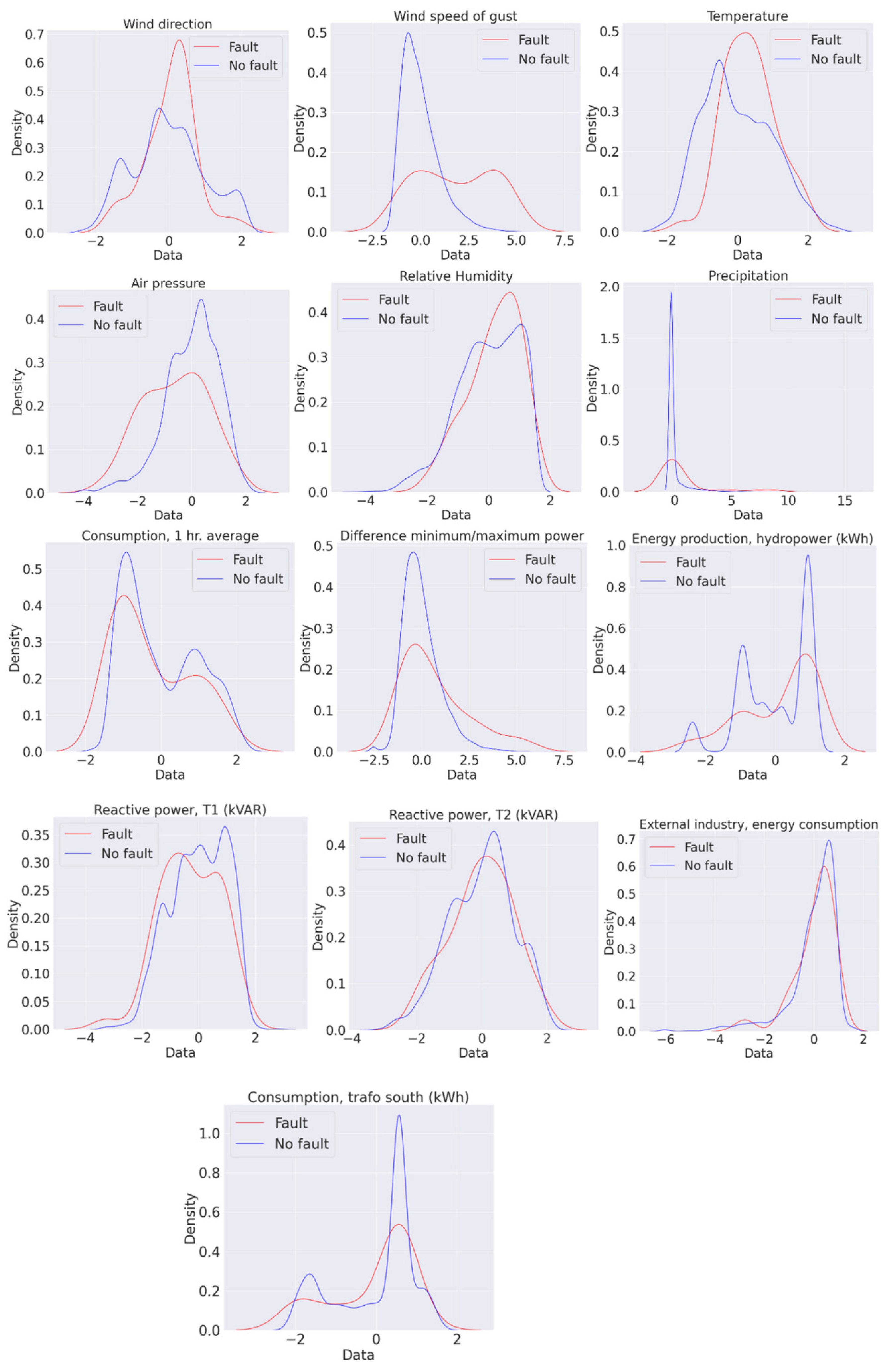
To gain an insight of the distribution of the values in each variable across the different classes, we use a Kernel Density Estimation (KDE) to estimate the distribution for each variable [40], as shown in Figure 6.

If the estimated density functions show significant differences between the failure class (red) and the normality class (blue), this indicates that a specific feature behaves differently in the two classes and can be used to discriminate among them. Looking at the distributions might help to assess which features are more important to identify the failures in the power grid. On the other hand, less important features have a similar distribution in both classes and are arguably less useful to discriminate among them.

It is clear from the density plots that it is very difficult to discriminate the minority from the majority class considering each feature individually, as the distributions are similar. From the density plots, it seems that wind speed is the most discriminating feature, since the distributions are different in the two classes.

To quantify the separation between the distributions numerically, we computed the Kullback–Leibler (KL) divergence. If the KL divergence is high, there is a large discrepancy between the two distributions [42]. The value of the KL divergence is given in

Table 3. KL divergence for each variable.

Variable	KL Divergence
Wind dir.	2.28
Wind speed	3.87
Temp.	2.21
Air pres.	1.61
Rel. Hum.	2.35
Precip.	0.82
Local industry: Energy consumption	3.83
Local industry: Diff. min/max power.	2.03
Energy production, hydropower	1.62
External industry: Reactive Power (T1)	3.58
External industry: Reactive Power (T2)	1.67
External Industry: Energy consumption	2.69
Consumption, Transformer south	3.83

.

The KL divergences confirm that wind speed is the most discriminating feature, as indicated from the distribution plots in Figure 5. However, from this analysis, it is difficult to verify that wind is the only feature causing failures in the SVAN22LY1 grid.

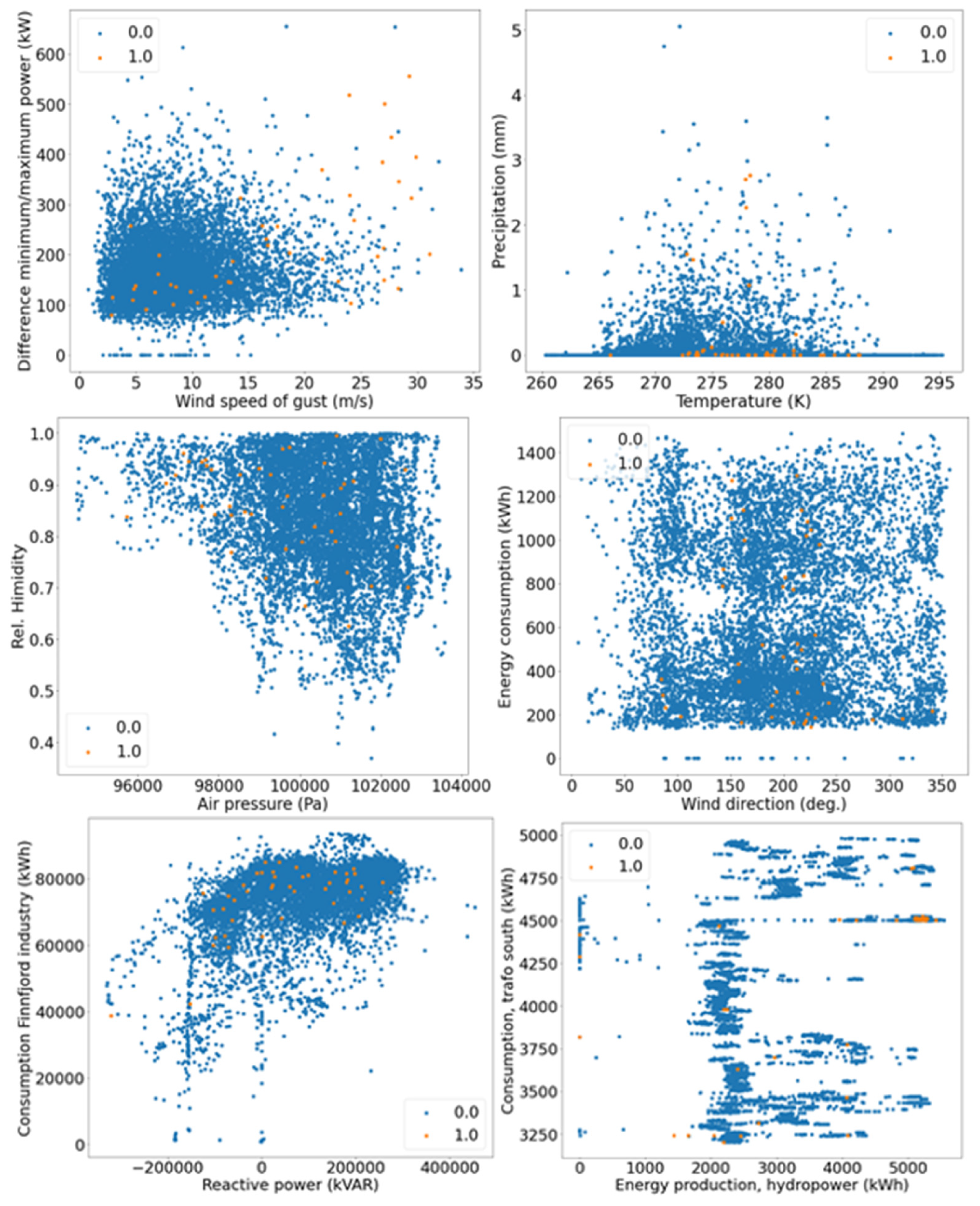
Visualization of Majority Class and Minority Class

Here, in addition to computing the KDE distribution (Figure 6) and the KL divergence (Table 3), the features are visualized as a scatter plot. The scatter plot provides an overview of how the two (minority and majority) classes are distributed for each feature. The scatter plot is given in Figure 7.

Figure 7 shows the two major challenges: class imbalance and non-trivial separation among classes.

The minority class (failures) is mixed with the majority class (normal conditions) repeatedly. However, the scatterplot of wind speed of gust shows that some failures are well separated from the rest. This indicates that the SVAN22LY1 power grid might experience more failures when there is a high wind speed of gust (above 25 m/s).

In summary, the difficulty in separating the two classes by using simple thresholds on the individual variables motivates the use of more advanced ML techniques.

6.2. Classification Performances

Here, the classification performances obtained by the different methods are compared. In

Table 4. Average classification performance for different models obtained across five different folds.

Classifier	TN	FP	FN	TP	Weighted F1 Score
Class-specific weights
Linear
Logistic Regression	1256	328	3	6	0.712
Ridge Classifier	1280	304	3	6	0.717
LinearSVC	1221	363	2	7	0.775
Non-linear
RBFSVC	1375	209	1	8	0.879
MLP	1301	283	1	8	0.860
SMOTE
Linear
Logistic Regression	1552	31	5	3	0.453
Ridge Classifier	1557	25	5	4	0.587
LinearSVC	1554	29	5	3	0.574
Non-linear
RBFSVC	1564	20	5	4	0.610
MLP	1543	40	5	4	0.605
One-class
One-class SVM	15	1568	1	7	0.576
Elliptic	14	1569	2	6	0.534
LOF	15	1568	1	8	0.615

, the performances of the different models are compared across the five folds in terms of the average number of TN, FP, FN, TP, and the weighted F1 score.

The results show that the non-linear SVC classifier (RBFSVC) with class weighting achieved top performance with a weighted F1 score of 0.879, which was followed by the MLP and the LinearSVC. The RBFSVC correctly classified eight out of the nine failures, resulting in a sensitivity score of 8/9 = 0.88 or 88%. Compared to use of class-specific weights, balancing the dataset with SMOTE results in a lower classification score for all models, and therefore, it is not a suitable method for this particular failure detection task. Interestingly, all the one-class models perform worse, as they find too many FP. A model that reports several FP (i.e., false alarms) is not useful in practice.

Finally, it is important to notice that the linear models achieve relatively good performance, which suggests that several data samples from the two classes are linearly separable. Therefore, a feature selection procedure is provided in Section 6.4.

6.3. Analysis of the Results

Here, a fixed train/validation/test split is generated and used. This ensures that the solution obtained by each model could be analyzed in detail. Since the RBBSVC classifier obtained the highest classification performance, the classification score for a fixed train/validation/test split was computed for this model. For this specific split, it is nine failures and 1398 non-failures in the test set. Here, the RBFSVC identified nine failures correctly while failing to classify three of the total amount of failures correctly.

To detect the possible causes for the nine failures in the test set, a closer investigation of the specific failures was performed in collaboration with the DSO. By investigating each failure individually, it was found that wind speed seems to be an important factor, as there were several days with failures where the wind was above 25 m per second. This is in line with the pre-analysis from the distribution plots and the KL divergence in Section 6.1, which shows that wind speed could be an important factor.

For one of the nine failures, no specific causes were identified. However, the official FASIT report for the specific incident shows that this failure was reported to be an earth failure [22].

Interestingly, the earth failure is one of the three false negatives. However, since it is independent of the weather and electricity load measure considered as input variables, it is correct that the SVM assigns it to the non-failure class and should not be considered as a true error.

In the end, out of nine failures in the test set, six failures were correctly detected with the ML model. Among the three false negatives, one failure was identified as earth failure, and for the two remaining failures wrongly classified, the cause remains unknown.

As the individual investigations of the nine failures showed that the magnitude of wind speed seems to be a causing variable, it would be of interest to categorize the different variables in terms of importance. This will provide knowledge regarding how the DSO could act in advance based on variables that are given as important and which variables are interpreted as less important.

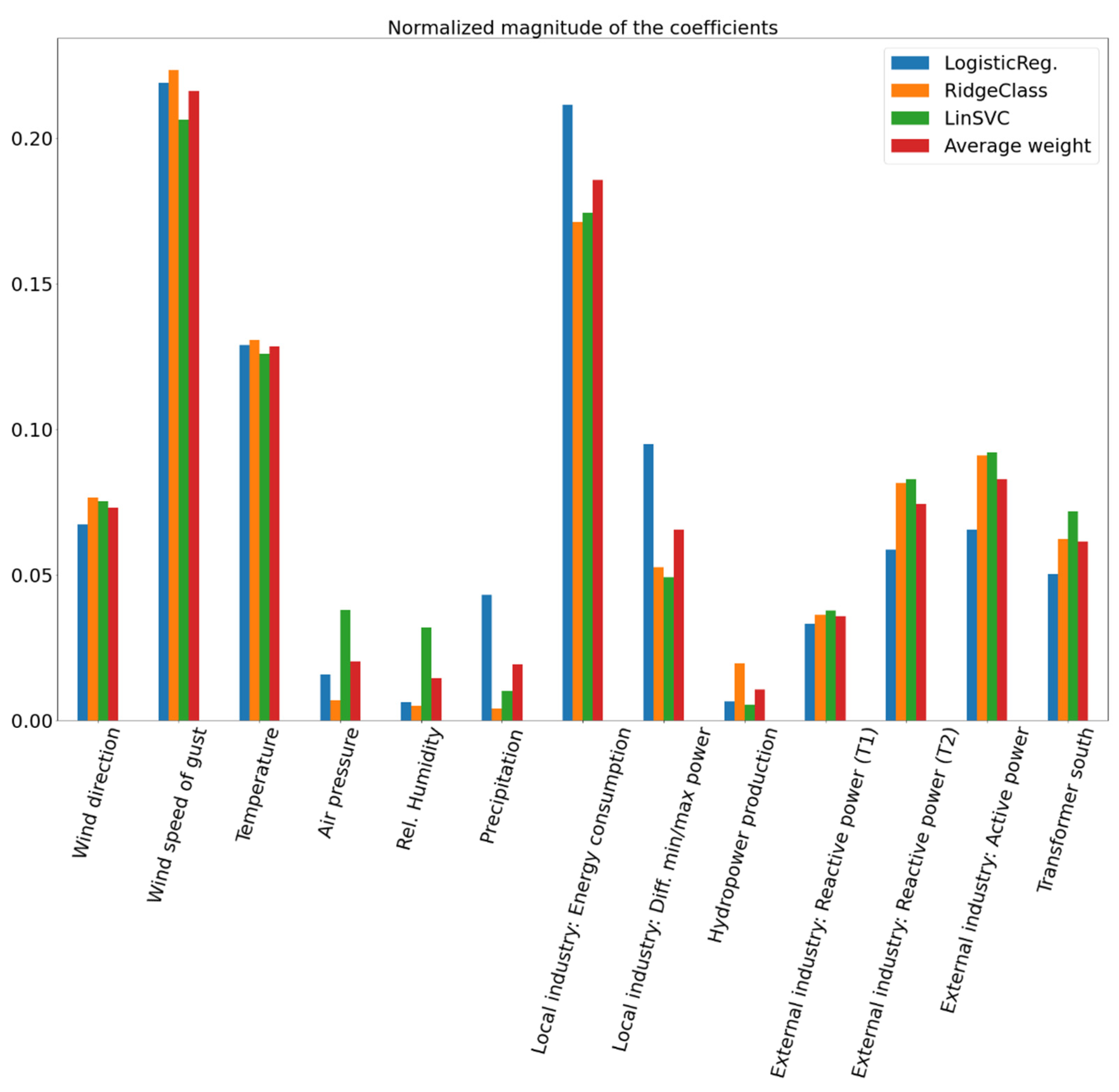
6.4. Identification of Important and Non-Important Features

To gain knowledge of which variables are the most relevant for causing failures in the power grid, it is possible to rank the different variables in terms of how much they contribute to explaining the classification results obtained by the ML models. As discussed in Section 5, looking at the magnitude of the weights attributed by the linear models to the input features allows us to identify the features that contribute the most to determining the correct class. In return, this can give insights about which variables mostly explain the occurrence of failures in the power grid. Figure 8 reports the magnitude of the weights assigned to each feature after each linear model is trained. In addition, the average weight of all linear models is reported for each feature. The higher the magnitude weight of a given feature is, the more such a feature is important in predicting the class.

From Figure 8, the wind speed of gust and energy consumption and the industries is given the highest weights, indicating that these features are the most important variables in discriminating between the failure and non-failure class. This confirms the pre-analysis from the Gaussian KDE distributions and KL divergences in Section 6.1. This is also in line with experiences from the DSO and local knowledge, which states that they often experience failures when the magnitude of wind is large, and there is a high activity at the industries with associated large strain on the power grid.

7. Conclusions

Failures have critical consequences for customers connected to the power grid, especially industries that are heavily dependent on having a stable power supply to avoid potential financial losses related to a power failure.

In this work, the problem of detecting such failures was addressed by using machine learning techniques. In collaboration with the local DSO, a dataset consisting of a wide spectrum of variables that could potentially explain power failures was constructed. The dataset consists of different power data and meteorological variables. Once the dataset was constructed, different machine learning classifiers were trained to detect power failures based on the value of the different variables in the constructed dataset.

The classification performance was compared in terms of the F1 score, and the RBFSVC classifier achieved the top performance with an F1 score of 0.879, where eight of nine failures in the test set were correctly detected. Among the linear models, the LinearSVC obtained the best result, with an F1 score of 0.775, and it correctly detected seven of the total nine failures. The good classification results obtained by the linear models motivated the interpretation of the decision process. Interpreting the decision process of a linear model is a valuable tool to identify the variables that mostly explain the power failure occurrence. The result of this interpretation technique shows that wind speed of gust and energy consumption at the local industry are the most important variables in explaining the power failures.

This interpretability technique allows us to gain deeper insight into the underlying causes of failures, and this type of knowledge is fundamental for the DSO that is operating the grid in our study. The DSO has so far not employed strategies to detect and interpret failures and has accepted the numerous failures that occur due to the fact that the causes remain elusive. Based on the findings in this work, the DSO can now develop better strategies for improving the power supply reliability.

Some examples of measures to enhance the power supply reliability are as follows: (i) changing the grid topology and making the grid more robust in areas where there is a higher likelihood that the grid could experience problems, (ii) introducing more electricity generation locally by installing renewable energy sources such as wind or solar energy, and (iii) developing a flexible market where the power loads in the grid can be controlled to ensure that the strain on the power grid is never too high. These strategies are being implemented by the DSO that operates the grid with the aim of reducing incoming failures. In addition, the DSO has recently connected a new battery system to the power grid. To improve the power supply reliability, this battery aims to be activated right before a power failure is expected to occur; thus, being able to predict these occurrences is important. Therefore, the findings in this study can be used by the DSO to better understand which variable should be monitored to detect an incoming power failure.

Limitations and Suggested Future Research

The interpretation technique identified the wind speed of gust as the most important feature in explaining the failure occurrence. The weather variables were collected from different regions in the power grid, and the AROME-Arctic model used to collect the data has a spatial resolution of 2.5 × 2.5 km. Therefore, the exact location of where the weather-related power failure might occur remains unknown. Suggested future work is to further narrow down the potential area where the weather most likely contributes to power failures. As the AROME-Arctic model has a coarse spatial resolution, a potential solution could be to install weather measurement stations in locations that are expected to be more exposed to weather-related failures. This will enable the possibility to have better and higher-resolution data available.

This interpretation technique allows us to find the main driving factors that, on average, contribute to power failures. However, while our interpretability is global, each individual fault occurrence might be caused by a different combination of parameters. We foresee future work aimed at developing a methodology that allows finding the causes of each individual failure, which will provide additional knowledge to the DSO.

References

- Chiaradonna, S.; Di Giandomenico, F.; Masetti, G. Analyzing the Impact of Failures in the Electric Power Distribution Grid. In Proceedings of the 2016 Seventh Latin-American Symposium on Dependable Computing (LADC), Cali, Colombia, 19–21 October 2016. [Google Scholar]
- Klinger, C.; Landeg, O.; Murray, V. Power Outages, Extreme Events and Health: A Systematic Review of the Literature from 2011–2012. PLoS Curr. 2014, 6. [Google Scholar] [CrossRef] [PubMed]
- Meles, T.H. Impact of power outages on households in developing countries: Evidence from Ethiopia. Energy Econ. 2020, 91, 104882. [Google Scholar] [CrossRef]
- Shuai, M.; Chengzhi, W.; Shiwen, Y.; Hao, G.; Jufang, Y.; Hui, H. Review on Economic Loss Assessment of Power Outages. Procedia Comput. Sci. 2018, 130, 1158–1163. [Google Scholar] [CrossRef]
- Forskrift om Leveringskvalitet i Kraftsystemet, Lovadata, 30 November 2004. Available online: https://lovdata.no/dokument/SF/forskrift/2004-11-30-1557 (accessed on 13 February 2021).
- Owerko, D.; Gama, F.; Ribeiro, A. Predicting Power Outages Using Graph Neural Networks. In Proceedings of the 2018 IEEE Global Conference on Signal and Information Processing (GlobalSIP), Anaheim, CA, USA, 26–29 November 2018. [Google Scholar]
- Hamachi LaCommare, K.; Eto, J.H. Cost of Power Interruptions to Electricity Consumers in the United States (U.S); Ernest Orlando Lawrence Berkeleley National Laboratory: Berkeley, CA, USA, 2006.
- Campbell, R.J. Weather-Related Power Outages and Electric System Resiliency. CRS Report for Congress 7-5700Weather-Related Power Outages and Electric System Resiliency (fas.org). 28 August 2012. Available online: https://sgp.fas.org/crs/misc/R42696.pdf (accessed on 27 December 2021).
- Gopinath, G.S.S.; Meher, M.V.K. Electricity a basic need for the human beings. In Proceedings of the International Conference on Renewable Energy Research and Education (RERE-2018), Andhra Pradesh, India, 8–10 February 2018. [Google Scholar]
- Tully, S. The Human Right to Access Electricity. Electr. J. 2006, 19, 30–39. [Google Scholar] [CrossRef]
- Csanyi, E. 4 Main Types of Distribution Feeder Systems to Recognize. Electrical Engineering Portal. 23 June 2016. Available online: https://electrical-engineering-portal.com/4-main-types-distribution-feeder-systems (accessed on 4 March 2021).
- NVE; Miljødirektoratet; ENOVA; Statens Vegvesen; Kystverket; Landbruksdirektoratet, Tiltak og virkemidler mot 2030. Klimakur 2030: Tiltak og virkemidler mot 2030—Miljødirektoratet (miljodirektoratet.no); The Norwegian Environment Agency: Oslo, Norway, 31 January 2020; Available online: https://www.miljodirektoratet.no/publikasjoner/2020/januar-2020/klimakur2030/ (accessed on 27 December 2021).
- Rubì, C. The Challenges of Upgrading the Power Grid for a decarbonised Electric Future. Informa Connect. 19 April 2019. Available online: https://informaconnect.com/the-challenges-of-upgrading-the-power-grid-for-a-decarbonised-electric-future (accessed on 4 March 2021).
- Arva Power Company. Troms Kraft. Available online: https://www.tromskraftnett.no (accessed on 1 March 2021).
- Xie, J.; Alvarez-Fernandez, I.; Sun, W. A Review of Machine Learning Applications in Power System Resilience. In Proceedings of the 2020 IEEE Power & Energy Society General Meeting (PESGM), Montreal, QC, Canada, 2–6 August 2020. [Google Scholar]
- Trakas, D.N.; Panteli, M.; Hatziargyriou, N.D.; Mancarella, P. Spatial Risk Analysis of Power Systems Resilience During Extreme Events. Risk Anal. 2018, 39, 195–211. [Google Scholar] [CrossRef] [PubMed] [Green Version]
- Sabouhi, H.; Doroudi, A.; Fotuhi-Firuzabad, M.; Bashiri, M. Electrical Power System Resilience Assessment: A Comprehensive Approach. IEEE Syst. J. 2020, 14, 2643–2652. [Google Scholar] [CrossRef]
- Perera, A.T.D.; Nik, V.M.; Chen, D.; Scartezzini, J.-L.; Hong, T. Quantifying the impacts of climate change and extreme climate events on energy systems. Nat. Energy 2020, 5, 150–159. [Google Scholar] [CrossRef] [Green Version]
- Panteli, M.; Mancarella, P. Influence of extreme weather and climate change on the resilience of power systems: Impacts and possible mitigation strategies. Electr. Power Syst. Res. 2015, 127, 259–270. [Google Scholar] [CrossRef]
- De Caro, F.; Carlini, E.; Villacci, D. Flexibility sources for enhancing the resilience of a power grid in presence of severe weather conditions. In Proceedings of the 2019 AEIT International Annual Conference (AEIT), Florence, Italy, 18–20 September 2019. [Google Scholar]
- Hoffmann, V.; Michalowska, K.; Andresen, C.A.; Torsæter, B.N. Incipient Fault Prediction in Power Quality Monitoring. In Proceedings of the CIRED Conference Proceedings, Madrid, Spain, 3–6 June 2019. [Google Scholar]
- Abusdal, G.M.; Heydt, G.T.; Ripegutu, A. Utilization of advanced metering infrastructure in back-fed ground fault detection. In Proceedings of the 2015 IEEE Power & Energy Society General Meeting, Denver, CO, USA, 26–30 July 2015. [Google Scholar]
- Andresen, C.A.; Torsaeter, B.N.; Haugdal, H.; Uhlen, K. Fault Detection and Prediction in Smart Grids. In Proceedings of the 2018 IEEE 9th International Workshop on Applied Measurements for Power Systems (AMPS), Florence, Italy, 26–28 September 2018. [Google Scholar]
- Arva Power Company. Final Report on Concept Study; Arva Power Company: Tromsø, Norway, 2019. [Google Scholar]
- Schiel, C.; Lind, P.G.; Maass, P. Resilience of electricity grids against transmission line overloads under wind power injection at different nodes. Sci. Rep. 2017, 7, 11562. [Google Scholar] [CrossRef] [PubMed] [Green Version]
- Csanyi, E. Detailed Overview of Power System Disturbances (Causes and Impacts). Eledtrical Engineering Portal. 17 April 2015. Available online: https://electrical-engineering-portal.com/detailed-overview-of-power-system-disturbances-causes-and-impacts (accessed on 4 March 2021).
- FASIT. FASIT, Statnett, 09 02 2021. Available online: https://www.statnett.no/for-aktorer-i-kraftbransjen/systemansvaret/leveringskvalitet/fasit (accessed on 3 March 2021).
- Kartverket. Hoydedata, Kartverket. Available online: https://hoydedata.no/LaserInnsyn (accessed on 3 March 2021).
- Geodetics. DEM, DSM & DTM: Digital Elevation Model–Why It’s Important, Geodetics. Available online: https://geodetics.com/dem-dsm-dtm-digital-elevation-models (accessed on 3 March 2021).
- The Norwegian Meteorological Institute. The AROME-Arctic Weather Model. The Norwegian Meteorological Institute. 2020. Available online: https://www.met.no/en/projects/The-weather-model-AROME-Arctic (accessed on 28 December 2020).
- Nguyen, H.M.; Cooper, E.W.; Kamei, K. Borderline over-sampling for imbalanced data classification. Int. J. Knowl. Eng. Soft Data Paradig. 2011, 3, 4–21. [Google Scholar] [CrossRef]
- Bishop, C.M. Pattern Recognition and Machine Learning; Springer: New York, NY, USA, 2006; 738p. [Google Scholar]
- Boser, B.E.; Guyon, I.M.; Vapnik, V.N. A training algorithm for optimal margin classifiers. In Proceedings of the Fifth Annual Workshop on Computational Learning Theory, Pittsburgh, PA, USA, 27–29 July 1992; pp. 144–152. [Google Scholar] [CrossRef]
- Goodfellow, I.; Bengio, Y.; Courville, A. Deep Learning; MIT Press: Boston, MA, USA, 2016. [Google Scholar]
- Khan, S.; Madden, M. One-class classification: Taxonomy of study and review of techniques. Knowl. Eng. Rev. 2014, 29, 345–374. [Google Scholar] [CrossRef] [Green Version]
- Schölkopf, B.; Platt, J.; Shawe-Taylor, J.; Smola, A.J.; Williamson, R.C. Estimating the Support of a High-Dimensional Distribution. Neural Comput. 2001, 13, 1443–1471. [Google Scholar] [CrossRef] [PubMed]
- Liu, T.F.; Ting, K.M.; Zhou, Z.-H. Isolation Forest. In Proceedings of the 2008 Eighth IEEE International Conference on Data Mining, Pisa, Italy, 15–19 December 2008. [Google Scholar]
- Hubert, M.; Debruyne, M.; Rousseeuw, P.J. Minimum covariance determinant and extensions. Wiley Interdiscip. Rev. Comput. Stat. 2018, 10, e1421. [Google Scholar] [CrossRef] [Green Version]
- Breunig, M.M.; Kriegel, H.-P.; Ng, R.T.; Sander, J. LOF: Identifying density-based local outliers. In Proceedings of the SIGMOD’00: Proceedings of the 2000 ACM SIGMOD International Conference on Management of Data, Dallas, TX, USA, 15–18 May 2000. [Google Scholar]
- Pedregosa, F.; Varoquaux, G.; Gramfort, A.; Michel, V.; Thirion, B.; Grisel, O.; Blondel, M.; Prettenhofer, P.; Weiss, R.; Dubourg, V.; et al. Scikit-learn: Machine Learning in Python. J. Mach. Learn. Res. 2011, 12, 2825–2830. [Google Scholar]
- Tensorflow. Tensorflow. And End-to-Ebd Open Source Machine Learning Platform. Available online: https://www.tensorflow.org (accessed on 5 November 2021).
- Alpaydin, E. Introduction to Machine Learning, 4th ed.; The MIT Press: Cambridge, MA, USA, 2020. [Google Scholar]