Article

Design and Implementation of an Intelligent Blade Pitch Control System and Stability Analysis for a Small Darrieus Vertical-Axis Wind Turbine

Mechanical and Mechatronics Engineering, University of Waterloo, Waterloo, ON N2L 3G1, Canada
*
Author to whom correspondence should be addressed.
Energies 2022, 15(1), 235; https://doi.org/10.3390/en15010235
Submission received: 14 November 2021 / Revised: 15 December 2021 / Accepted: 28 December 2021 / Published: 30 December 2021
(This article belongs to the Collection Wind Turbines)

Abstract

:
A few studies have been conducted recently in order to improve the aerodynamic performance of Darrieus vertical-axis wind turbines with straight blades (H-type VAWTs). The blade pitch angle control is proposed to enhance the performance of H-type VAWTs. This paper aims to investigate the performance of an H-type VAWT in terms of its power output and self-starting capability using an intelligent blade pitch control strategy based on a multi-layer perceptron artificial neural network (MLP-ANN) method. The performance of the proposed blade pitch controller is investigated by adding a conventional controller (PID) to the MLP-ANN controller (i.e., a hybrid controller). The dynamics of an H-type VAWT is mathematically modeled in a nonlinear state space for the stability analysis in the sense of Lyapunov. The effectiveness of the proposed pitch control system is validated by building an H-type VAWT prototype model that is extensively tested outdoors under different conditions for both fixed and variable pitch angle configurations. Results demonstrated that the blade-pitching technique enhanced the power output of an H-type VAWT by approximately 22 % . The hybrid controller that used a high percentage of the MLP-ANN controller achieved a better control performance by reducing the overshoot of the control response at high rotor speeds.

1. Introduction

Stand-alone power supply systems, such as wind turbines, are not only suitable solutions for producing the electricity needed for rural and remote areas, but also economical alternatives because they can contribute to a reduction in the cost of grid extensions [1]. For a number of years, two main types of wind turbines have been adopted for the extraction of power from wind: horizontal-axis wind turbines (HAWTs) and vertical-axis wind turbines (VAWTs). VAWTs offer a number of advantages over HAWTs: VAWTs can receive wind blowing from any direction (i.e., omni-directional) so that a yaw mechanism is unnecessary; the simplicity of the blade design means that the cost is relatively low [2]; and VAWT maintenance is comparatively quick and easy because the transmission equipment and generator are located at ground level [3]. VAWTs fall into two different categories: (1) the Savonius rotor, which is a drag-type device, and (2) the H-Darrieus rotor, which is a lift-type device in which the blades are straight and parallel to the axis of rotation with a fixed or variable pitch angle [3]. An important parameter associated with VAWT blades is the operating tip speed ratio (TSR), λ . A key factor in the selection of the TSR is wind speed, as given in [4]:
λ = ω r R u ,
where ω r is the angular velocity of the rotor, u is the wind speed, and R is the rotor radius. The actual VAWT performance can be predicted based on a determination of the forces acting on each blade. Figure 1 illustrates the velocity and force vectors acting on a Darrieus turbine blade. The velocity V is the tangential velocity vector of the rotor. The resultant velocity vector W is the relative velocity, which consists of the induced velocity U and V . The angle of attack α is typically defined as the angle between the direction of the relative velocity, W , and the chord line of the blade. The blade pitch angle is described in [5]:
β = α φ ,
where φ is the angle between the direction of V and W . Obviously, the angle of attack α varies during each cycle. The result is that the magnitude and orientation of both the lift and drag forces change depending on the azimuthal position of the blade θ . Figure 1 also shows the main forces acting on a VAWT blade; namely, the lift, drag, normal N, and tangential T forces.
However, for VAWTs at low TSRs, a negative torque is often generated because of the large dynamic cyclic variations in the angle of attack α . The angle of attack α for a VAWT with a fixed pitch angle (viz., β = 0 ) can be expressed as follows [6]:
α = tan 1 cos θ sin θ + λ .
To improve the VAWT performance, a variable pitch technique is applied through the modification of the angle of attack α . A variable pitch angle control system can be either of two main categories: passive or active [7]. In a passive variable pitch system, the blade is free to pitch about its axis near the leading edge. Theoretically, a passive pitch system can greatly improve the starting torque and performance of a VAWT. However, experimental analysis has shown that the maximum power value is less than a third of the predicted value [6]. In an active control system, pitch control mechanisms, such as pushrods, or cams have been designed to achieve continuous changes in the blade pitch amplitude [8].
At low TSRs, a large pitch amplitude is needed in order to reduce the angle of attack and, hence, to enhance the rotor performance. However, a large pitch amplitude can cause the VAWT performance to deteriorate at high TSRs. Conversely, while a small pitch amplitude is sufficient for producing good performance at high TSRs, it will lead to poor performance at low TSRs [6,9]. This effect gives rise to an important question: How should the pitch amplitude be varied in order to optimize the VAWT performance as the TSR changes? A suitable aerodynamic model for determining the optimum pitch angle and a control system that can approximate the optimal pitch angle of an H-type VAWT during rotation are therefore required.
Self-starting definition: Under a no-load condition and stationary blades, the Darrieus VAWT can generate a small amount of forward torque and, hence, can start to rotate slowly. As a result of negative torque, the extracted power per cycle is less than zero typically at low tip speed ratios depending on the blade airfoil [10]. Therefore, the Darrieus VAWT cannot accelerate up in order to generate any power output. As a result, an external power, such as a motor, is required to accelerate the rotor up, and, hence, to generate power [11]. Hill et al. [12] opined that there is no exact definition for the term self-starting. Many studies, however, suggest some criteria to define the term of self-starting, such as, for example, the ability of the rotor to accelerate from rest to its nominal operating speed without external power [13], which is used in this paper. Therefore, the small amount of power production by the H-type VAWT at low TSRs (i.e., an useful power) is defined as the self-starting capability.
Although VAWTs have been in existence for many years, very limited research has been conducted with respect to these systems, in comparison to the more extensive investigations devoted to HAWTs [14].
Numerous studies have suggested a variety of pitch angle control methods. The proportional-integral (PI) or proportional-integral-derivative (PID)-based pitch angle controllers have been used for power regulation. Unfortunately, these linear control methods offer only a limited performance, especially in the face of the uncertainties associated with the nonlinear dynamic properties of wind turbines [15]. A linear quadratic Gaussian (LQG) control method has also been applied for pitch angle control. Although it is a more robust method compared to the PID control method, its performance is also limited with respect to its applicability to a nonlinear system [15]. Sliding-mode control techniques have also been applied to pitch angle control. These techniques provide a robust performance, but require an observer to estimate the aerodynamic torque and rotor acceleration [16]. Intelligent control techniques that employ approaches such as neural networks and fuzzy logic have also been proposed for the modeling and control of nonlinear dynamical systems [17,18]. These methods are powerful when the system contains a high nonlinearity due to effects such as strong wind turbulence. However, all of the above research related to pitch control systems has been conducted for HAWTs.
Although an artificial intelligence strategy based on the ANN and fuzzy expert system (FES) method is used for VAWTs [19,20], these methods are used only for predicting the power output of VAWTs. To the best of the authors’ knowledge, the published literature contains no studies related to the intelligent control of the pitch angle for Darrieus VAWTs.
H-type VAWT models are nonlinear because the rotor efficiency, which is dependent on the rotor speed, the wind speed, and the blade pitch angle, is highly nonlinear. Therefore, linear control methods alone are not usually sufficient for ensuring the desired performance in terms of the power output and self-starting capability. Some studies [21,22] have attempted to combine neural networks with conventional controllers, such as PI or PID, to develop a stable and robust control system for handling nonlinear system dynamics.
The objective of the work presented herein is to systematically design an intelligent nonlinear individual active blade pitch control system for a small H-type VAWT.
In this paper, the three blades of the H-type VAWT are controlled individually using both global MLP-ANN and PID controllers (hybrid controller), which will be shown to improve the power generation performance of the VAWT.
If each blade can be controlled individually, it is possible to maximize the moment coefficient for all blades. The wind turbine performance can be optimized by predicting the optimum blade pitch angle in order to generate the highest value of torque. The authors in [23] analyzed a 1.7 m diameter 2D three-bladed H-type VAWT with a variable pitch angle and NACA 0018 airfoil numerically using computational fluid dynamics (CFD). This analysis was carried out for pitch angles of β = 6 , 4 , 0 , 4 , and 6 ; TSRs of λ = 1 , 1.7 , 2, 2.5 , and 3.3 ; and, a mean wind speed of u = 10 m/s. ANSYS-Fluent software was used to conduct a series of CFD simulations in order to estimate the moment coefficients C m at each rotor position for each blade. The power coefficient C p , which represents the efficiency of a wind turbine, is calculated for each individual blade as follows:
C p = C m λ ,
The maximum moment coefficient C m , max was determined at each rotor position θ in order to define the optimum blade pitch angle β opt . These optimal pitch angles were utilized in the design of the proposed blade pitch control system in the numerical simulink model. To validate both CFD and MATLAB Simulink simulation results in [23], a H-type VAWT prototype is built to test the effectiveness of the proposed pitch control system that is presented in this paper.

2. An H-Type Vawt Modeling

Describing the dynamic wind turbine model mathematically for each component has been investigated in a number of studies [24,25,26,27]. The main components of an H-type VAWT are shown in Figure 2. The wind turbine characteristics that will be considered in this section are: aerodynamics, turbine mechanics, generator dynamics, and actuator dynamics.

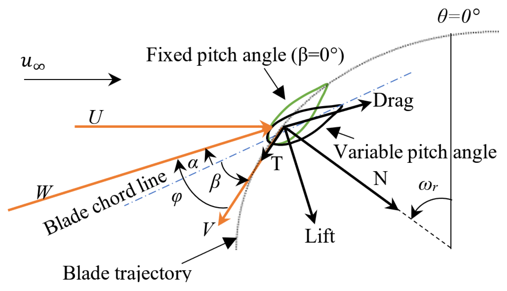
2.1. Aerodynamic Block

The power extracted from the wind can be expressed as follows [28]:
P W = 1 2 ρ A u 3 ,
where ρ is the air density, and A is the area swept by the turbine (e.g., for the H-type Darrieus wind turbine, A = 2 R H , where H is the blade length). In fact, only a fraction of this power can be captured by the turbine, representing the mechanical power P m generated by the wind turbine rotor, which is determined as follows:
P m = 1 2 ρ A u 3 C p ( λ , β ) ,
The amount of aerodynamic torque τ r generated by the rotor in N·m is given by
τ r = P m ω r .

2.2. Mechanical Block

This block is represented in wind turbine models using a two-mass drive-train model, as shown in Figure 3. By using a free-body diagram, the torque about a shaft can be determined from
τ = J θ ¨ + D θ ˙ + K θ ,
where θ is the azimuth angle. By applying Equation (8) to all four rotating masses, the drive-train can be modeled as follows:
J r θ ¨ r + D L S ( θ ˙ r θ ˙ L S ) + K L S ( θ r θ L S ) + D r θ ˙ r = τ r
J g θ ¨ g + D H S ( θ ˙ g θ ˙ H S ) + K H S ( θ g θ H S ) + D g θ ˙ g = τ g
J r θ ¨ L S D L S ( θ ˙ r θ ˙ L S ) K L S ( θ r θ L S ) = τ L S
J g θ ¨ H S D H S ( θ ˙ g θ ˙ H S ) K H S ( θ g θ H S ) = τ H S ,
where, J r and J g are, respectively, the moments of inertia of the wind turbine rotor and the generator in kg-m 2 ; τ r and τ g are, respectively, the wind turbine aerodynamic and generator electromagnetic torque in N·m; θ r and θ g refer to the angular position of the rotor and the generator in radians, respectively; θ ˙ r and θ ˙ g represent the wind turbine rotor and the generator speeds in rad/s, respectively; and θ ¨ r and θ ¨ g are their derivatives. Similarly, all of the above parameters are defined in terms of either the higher or lower shafts (HS and LS) of the wind turbine drive-train. Finally, D H S and K L S are the equivalent damping and stiffness coefficients for the higher and lower shafts in N·m·s/rad and N·m/rad, respectively.
Assumptions [25,26,27]:
  • The θ ¨ L S and θ ¨ H S terms are equal to zero because of their direct coupling inside the gear box;
  • The rotor and generator self-damping D r and D g are neglected.
Rearranging Equations (9)–(12), it can be seen that there are two state equations:
J r θ ¨ r = τ r τ L S ,
J g θ ¨ g = τ g + τ H S
However,
k = τ L S τ H S = θ ¨ g θ ¨ r ,
where k is the gear ratio. Now, Equations (13) and (14) can be simplified using Equation (15) as follows:
J r θ ¨ r + k J g θ ¨ g = τ r k τ g τ L S + k τ H S .
Then, dividing this equation by θ ¨ r gives
J r θ ¨ r θ ¨ r + k J g θ ¨ g θ ¨ r = τ r k τ g θ ¨ r ,
J r + k 2 J g = τ r k τ g ω ˙ r ,
implying that
ω ˙ r = τ r k τ g J t o t .
The total equivalent moment of inertia of the drive system is
J t o t = J r + k 2 J g .

2.3. Pitch Actuators

The actuator is modeled as an integrator. The dynamic model of the pitch actuator can be described as [29]:
β ˙ = 1 τ β β c 1 τ β β ,
where β and β ˙ are the actual pitch angle and its temporal derivative, respectively. These quantities are modulated by the time constant τ β . It is assumed that β c , which is a control signal, is equal to β , owing to the fact that the dynamics of the pitch system operates much faster than that of the mechanical system [15,30].

2.4. Nonlinear State-Space Representation of the System

The rotor angular velocity ω r is chosen for the system as the system state variable, and the pitch angle β c is the input control variable. A model of the H-type VAWT system can be described using Equations (19) and (21). The nonlinear affine model of the system is formulated as
{ x ˙ = f ( x ) + g ( x ) u , y = h ( x ) ,
where x and u are the state and input vectors, respectively, with
x = ω r β , u = β c , g ( x ) = 0 1 t β ,
and
f ( x ) = τ r k τ g J t o t 1 t β β = 1 2 ω r J t o t ρ A u 3 C p ( λ , β ) k τ g J t o t 1 t β β
= 1 2 x 1 J t o t ρ A u 3 C p ( λ , β ) k τ g J t o t 1 t β x 2 .

3. Stability Analysis of an H-Type VAWT

The stability of equilibrium points is usually characterized in the sense of Lyapunov (a Russian mathematician).

3.1. Lyapunov Stability

Consider a dynamical system that satisfies
x ˙ = f ( x ) .
Now, x ¯ R n is an equilibrium point of Equation (23) if f ( x ¯ ) 0 (i.e., the equilibrium point is a zero of f ( x ) ). This equilibrium point is locally stable if all solutions that are initialized in the vicinity of x ¯ remain in the vicinity of x ¯ (implying that the solutions remain in a neighborhood of x ¯ ); otherwise, it is unstable. The equilibrium point is locally asymptotically stable if all solutions starting at nearby points not only stay nearby, but also tend to the equilibrium point as time approaches infinity (viz., as t ).

3.2. Lyapunov’s Direct Method

Lyapunov’s direct method provides a number of theorems for establishing the local or global stability of a system. In order to proceed, the concept of a Lyapunov function will need to be considered [31].
Definition 1
(Lyapunov function). Let B ϵ be a ball of size ϵ around the origin. If, in a ball B ϵ , the function V ( x ) is positive definite and has continuous partial derivatives, and if its time derivative along any state trajectory of the system x ˙ = f ( x ) is negative semi-definite, then V ( x ) is said to be a Lyapunov function for the system.
Theorem 1
(Local stability). An equilibrium state exhibits local stability if:
  • V ( x ) is positive definite locally in B ϵ ;
  • V ˙ ( x ) is negative semidefinite locally in B ϵ .
The equilibrium is asymptotically stable if V ˙ ( x ) is negative definite.
Theorem 2
(Global stability). For the equilibrium state to be globally (asymptotically) stable, the ball B ϵ must include the whole state-space. Furthermore, V ( x ) must be radially unbounded. In other words,
  • V ( x ) is positive definite;
  • V ˙ ( x ) is negative definite;
  • V ( x ) →∞ as | | x | | →∞.
The above theorems provide a conceptually simple method for analyzing a system for stability. However, the drawback with this approach is that there is generally no systematic method for finding a Lyapunov function V ( x ) . Furthermore, the theorems do not provide any information about the instability of an equilibrium point [32].
In fact, there are no general procedures for selecting a suitable Lyapunov function for a given dynamical system. However, the stability property of the system can be predicted by using the actual energy function of the system. In particular, the Lyapunov function can be found by replacing the energy-like function with the actual energy function in the stability analysis of a dynamical system [32].
In this paper, the stability of equilibrium points of the closed-loop system [cf. Equation (22)], is addressed for a variable pitch angle H-type VAWT by using the Lyapunov stability theory.
In the next section, the equilibria points for the closed-loop system with a constant pitch angle ( β = 0 ) will be obtained. Subsequently, the stability for the variable pitch angle case will be analyzed.

3.3. Constant Pitch Angle Model

For HAWTs, the stability of the system was examined in [25,26,27]. These references used a standard control strategy for the generator torque control as follows:
k τ g = k t ω r 2 , k t > 0 .
The control gain parameter k t is given by:
k t = 1 2 ρ A R 3 C p λ 3 .
For the optimum case (viz., at the maximum C p value),
k t = 1 2 ρ A R 3 C p , o p t λ o p t 3 .
These investigations also demonstrated that if the curve
C p , c u b i c = 2 k t ρ A R 3 λ 3
intersects the C p λ curve at points λ 1 and λ 2 , as shown in Figure 4, then the equilibrium point ( C p , e q , λ 2 ), with C p , e q = 2 k t ρ A R 3 λ 2 3 , is asymptotically stable with a domain of attraction λ ( λ 1 , ) . However, k t is used in a specific range to guarantee the stability of the equilibrium point ( C p , e q , λ 2 ). Figure 4 also shows that the upper bound of k t occurs when Equation (25) is tangential to the C p λ curve. With respect to this limiting equilibrium point, ( C p , e q , λ 2 ) is stable if the slope of the C p λ curve at that point satisfies the following constraint [26]:
C p λ | ( C p , e q , λ 2 ) < 3 C p , e q λ 2 .

3.4. Variable Pitch Angle Model

The primary control objective of this study is to maximize the power output using blade pitching. The torque control law can be formulated as follows [24,26,27]:
τ g = P ref k ω r ,
where P ref is a constant rated power. From Equation (19), the closed-loop equation is
J t o t ω ˙ r = τ r P ref ω r .
For a constant wind speed operation, using the Equation (1) derivative and inserting Equation (7) into Equation (30) yields
J t o t λ ˙ u R = P m ω r P ref ω r ,
from which, it follows that
λ ˙ = R u 2 J t o t ω r 1 2 ρ A C p ( λ , β ) P ref u 3 .
Assumption 1
In order to examine the stability of an operation for a variable pitch angle H-type VAWT, it is assumed that the equilibria satisfy [26]:
C p λ < 0 ,
and
C p β < 0 for β β 0 and β 0 = 0 .
For each blade, the nonlinear pitch control (hybrid control) law for an H-type VAWT is given by
β = β ( M L P A N N ) + β P I D .
The following assumptions are made in order to facilitate the stability analysis of the proposed H-type VAWT:
  • The error e for both the PID and MLP-ANN controllers are similar with
    error = e = ω r 2 ω r , ref 2 ;
  • A single-input single-output (SISO) MLP-ANN with one hidden layer is proposed for the stability analysis of an H-type VAWT. The control law for the MLP-ANN controller is given by
    β ( M L P A N N ) = ϕ ( e ) = ϕ ω r 2 ω r , ref 2 ,
    where ϕ is the nonlinear transformation of the error (signal) e (input of the SISO MLP-ANN) provided by the neural network.
Furthermore, the PID control law is given by
β P I D = k p ω r 2 ω r , ref 2 + k d t ω r 2 ω r , ref 2
+ k i t 0 t ω r 2 ω r , ref 2 d t .
The linear control will be simplified to a PI controller because the derivative of the error in Equation (36) is very small, so
β P I D = β P I = k p ( ω r 2 ω r , ref 2 ) + k i t 0 t ( ω r 2 ω r , ref 2 ) d t .
By substituting Equations (35) and (37) into Equation (33), the pitch control law for each blade becomes
β = ϕ ω r 2 ω r , ref 2 + k p ω r 2 ω r , ref 2
+ k i t 0 t ω r 2 ω r , ref 2 d t .
For two steady wind speeds u , 1 and u , 2 , the resulting equilibrium points A and B occur at the intersections of the C p ( λ , β ) curve with the cubic curve C p , c u b i c = 2 k t ρ A R 3 λ 3 , as shown in Figure 5. Now,
γ = λ 2 2 γ ˙ = λ λ ˙ .
Substituting Equations (1) and (32) in Equation (39) leads to
γ ˙ = ω r R u R u 2 J t o t ω r 1 2 ρ A C p ( λ , β ) P ref u 3 = K L ,
where
K = R 2 u J t o t , L = 1 2 ρ A C p ( λ , β ) P ref u 3 .
The dynamics of the error variable γ ˜ can be defined as follows [26,27]:
γ ˜ = γ γ eq ,
where γ eq = λ eq 2 2 and λ eq could be equal to either λ E , 1 or λ E , 2 (cf. Figure 5). Then,
γ ˜ = λ 2 2 λ eq 2 2 γ ˜ ˙ = λ λ ˙ = K L .
The stability of the equilibrium at γ ˜ = 0 needs to be investigated. The error in Equation (34) needs to be quantified at the equilibrium point. To this purpose, if we take the time derivative of β in Equation (38) and let ω r , ref = ω r , eq , and, using Equation (1), we obtain
β ˙ = 2 ϕ ω r ω ˙ r + 2 k p ω r ω ˙ r + k i ( ω r 2 ω r , eq 2 ) ,
where ϕ d ϕ / d e . Now, observe that
β ˙ = 2 ϕ u R 2 λ λ ˙ + 2 k p u R 2 λ λ ˙ + 2 k i u R 2 γ ˜ .
Now, substituting for λ λ ˙ from Equation (42) gives
β ˙ = 2 ϕ u R 2 γ ˜ ˙ + 2 k p u R 2 γ ˜ ˙ + 2 k i u R 2 γ ˜ .
Furthermore, taking the time derivative of Equation (42) yields
γ ˜ ¨ = K L λ λ ˙ + K L β β ˙
= K L λ γ ˜ ˙ λ + K L β ( 2 ϕ u R 2 γ ˜ ˙ + 2 k p u R 2 γ ˜ ˙
+ 2 k i u R 2 γ ˜ ) .
This can be further recast to give
γ ˜ ¨ = K L λ 1 λ + K L β 2 ϕ u R 2 + 2 k p u R 2 γ ˜ ˙
+ 2 k i K L β u R 2 γ ˜
γ ˜ ¨ + f ( λ , β ) γ ˜ ˙ + g ( λ , β ) γ ˜ = 0 ,
where
f ( λ , β ) = ( K L λ 1 λ + K L β ( 2 ϕ u R 2
+ 2 k p u R 2 ) )
and
g ( λ , β ) = 2 k i K L β u R 2 .
In order to proceed further with the stability analysis, we need an explicit form for ϕ . To this purpose, the simplest architecture for a SISO MLP-ANN controller consists of a single hidden neural unit with a sigmoidal (logistic) activation function σ ( z ) 1 / ( 1 + exp ( z ) ) . Assuming that the activation function for the output neural unit is linear, the nonlinear transformation of the input error signal e for this SISO MLP-ANN controller is ϕ ( e ) = w ( 2 ) σ ( w ( 1 ) e ) , where w ( 1 ) and w ( 2 ) are the weights from the input neuron to the hidden neuron and from the hidden neuron to the output neuron, respectively. It is assumed that these weights (gains) are positive. From this, it follows that
ϕ ( e ) = w ( 1 ) w ( 2 ) σ ( w ( 1 ) e ) 1 σ ( w ( 1 ) e ) .
From Equations (39), (46) and (47), Assumption 1, and the definitions of L, f ( λ , β ) , and g ( λ , β ) , the nonlinear model for a variable pitch angle H-type VAWT system can be characterized as follows:
f ( λ , β ) = κ [ K C p ( λ , β ) λ 1 λ
+ K C p ( λ , β ) β 2 w ( 1 ) w ( 2 ) σ ( 1 σ ) u R 2 + 2 k p u R 2 ] > 0 ;
and,
g ( λ , β ) = 2 κ k i K C p ( λ , β ) β u R 2 > 0 ,
where κ 1 2 ρ A .
Now, the Lyapunov function candidate (viz., the energy-like function) can be defined as follows [26,32,33]:
V = 1 2 γ ˜ ˙ 2 + 0 γ ˜ g ( λ , β ) γ ˜ d γ ˜ .
Note that V is positive definite. The derivative of V along the system trajectories of Equation (48) is:
V ˙ = γ ˜ ˙ γ ˜ ¨ + g ( λ , β ) γ ˜ γ ˜ ˙ = f ( λ , β ) γ ˜ ˙ 2 0 .
It can be seen that V ˙ is semi-negative definite. Based on Theorem 1, it can be concluded that γ ˜ = 0 is locally stable at λ eq . Although the stability of the control law in Equation (33) is proven in the sense of Lyapunov, the asymptotic stability for the equilibrium point still needs to be established. In order to investigate the asymptotic stability condition, LaSalle’s invariance principle is utilized. The theorem states that if there are no system trajectories that can stay forever at points where V ˙ = 0 , except at the origin (equilibrium point), then the origin is asymptotically stable [31].
Let S = { x D | V ˙ ( x ) = 0 } , and suppose that no solution can stay forever in S, other than the trivial solution. Then, the origin is asymptotically stable. To characterize the set S for Equation (49), note that
V ˙ = 0 f ( λ , β ) γ ˜ ˙ 2 = 0 γ ˜ = 0 ( i.e. , λ = λ eq ) .
Therefore, the only solution that can stay in S for all t is the trivial solution. Thus, the origin ( γ ˜ = 0 , γ ˜ ˙ = 0 ) is asymptotically stable (or, equivalently, the equilibrium point λ eq is asymptotically stable).

4. Experimental Validation

The effect of blade pitching on an H-type VAWT in terms of both the power output and self-starting capability has been numerically investigated [23]. The results showed that the power output and self-starting capability are increased by 25% and 12%, respectively. In order to validate these results, a full-scale H-type VAWT with a blade pitching capability was constructed to examine the performance of the proposed hybrid pitch control system. The manufacturing and assembly phase consisted of five key stages: blade fabrication (NACA 0018), blade hub and linkage manufacturing, main shaft and bearing setup, generator and main shaft coupling, and, finally, the overall assembly of all these components, as shown in Figure 6.

Design and Implementation of the Proposed Blade Pitch Control System

Figure 7 shows a diagram of the overall experimental setup of the H-type VAWT used for validating the effectiveness of the proposed blade pitch control system.
The hybrid controller proposed in this work consists of MLP-ANN and PID controller combinations, as shown in Figure 7. The MLP-ANN and PID controllers used the pitch angle error e as an input signal produced by a comparison between the reference obtained from the CFD results and the actual pitch angle. A multiple-input single-output (MISO) MLP-ANN is proposed for designing an active intelligent blade pitch control system for an H-type VAWT. The error e, its derivative e ˙ , the reference pitch angle β ref , and the azimuth angle θ are used as inputs to the proposed MLP-ANN controller, whereas the output consists of the pitch angle additive command to supplement the linear control command for each blade, as shown in Figure 8.
MLP-ANN structure [23]: For each blade, the intelligent pitch angle control system consists of a fully connected three-layer feedforward MLP-ANN. The numbers of nodes in the hidden and output layers are 20 and 1, respectively. The sigmoid function is used as the activation function for neurons in the hidden layer. The Levenberg–Marquardt (LM) backpropagation algorithm is used to “learn” the weights of the MLP-ANN controller [34]. This training process consists of executing the LM algorithm for 1000 epochs over the data set.
Table 1 shows the parameters for the PID controller for each blade, which are tuned manually. The output of the MLP-ANN is then combined with the output of the PID to provide the final control command to each blade.
The reference pitch angle variations are sometimes small, with the result that the controller is unable to track them. Therefore, these small changes are adjusted to be greater than or equal to 4 . In addition, the sharp edges due to the pitch angle changes are also smoothed for each blade. Figure 9 shows a comparison between the original and the new adjusted reference pitch angles.
For each blade, the pitch angle is controlled by a closed loop hybrid controller, which sets a reference angle for each blade according to the instantaneous rotor angle θ . Then, the hybrid controller tries to set the actual blade pitch angle, measured by the blade encoder, in order to track the reference signal (i.e., reference pitch angle) with minimal error. Each blade angle is controlled independently using a four-bar linkage actuated by a DC motor.
Figure 10 shows the DC motor aluminum housing, stopper, and two limit switches, which are placed at both sides of the stoppers to limit the measured pitch angles to be between 6 and 6 . These switches are mounted under the lower linkage for each blade. The blade encoder (potentiometer) is mounted at the end of the effector-blade and is used as a position feedback sensor.
The H-type VAWT prototype is equipped with a data acquisition system (DAQ) for data logging and interfacing the hardware to software, which uses a virtual instrument (VI) developed using LabVIEW software. Some parameters, such as the wind speed, the rotor speed (RPM), the actual pitch angles, and the PMSG current and voltage, are measured by using specific sensors that are interfaced with the DAQ system.

5. Experimental Results
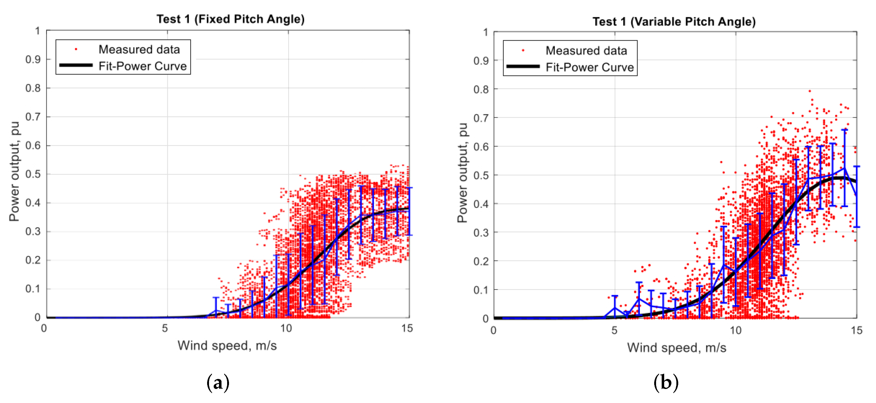
The H-type VAWT, including the pitch control system, is extensively tested outdoors for both fixed and variable blade pitch configurations. The outdoor trials are divided into three main experimental tests based on the purpose of the test. A preliminary test is conducted to examine the mechanical structure of the H-type VAWT prototype. In the first test, the power output, the self-starting capability, and the proposed control effectiveness of the H-Type VAWT prototype are investigated. To confirm the findings, the second test is performed by repeating the first test under different conditions. The operational reliability of the H-type VAWT is monitored in the preliminary test, which showed that the H-type VAWT mechanical structure is stable at different rotor speeds, ranging from 18 to 48 RPM, corresponding to a high aerodynamic disturbance condition. In this paper, the results and analysis of the first test are presented.

5.1. Power Curve

The measured power output for wind turbines at different wind speeds is encapsulated by a power curve that characterizes the efficiency of the wind turbine. For both fixed and variable pitch angle configurations, the power generation in pu (per unit) versus the wind speed in m/s for the H-type VAWT is shown in Figure 11.
For a variable pitch angle, the H-type VAWT produces a higher power output at wind speeds greater than 10 m/s compared to the fixed pitch angle case. Furthermore, a small amount of power output at wind speeds ranging from 4 m/s to 7 m/s is produced by the H-type VAWT. This implies that both the power output and the self-starting capability is enhanced by using the proposed blade pitching technique. The measured power output is fitted using the MATLAB Curve Fitting tool to generate the nonlinear curves (black curves) for both cases, as shown in Figure 11.
Figure 12 shows the filtered power generation curve for the fixed and variable pitch angle configurations. For data filtering, a moving-average filter is used here to reduce the power fluctuations (which consisted of determining running averages along all of the data streams for all of the cases). Moreover, any instantaneous power output less than or equal to zero is rejected. The areas below all of the power curves displayed in Figure 12 represent the total gross energy harnessed by the H-type VAWT for the fixed and variable pitch cases. Numerical integration using the trapezoidal rule is performed to calculate the total gross energy. The results showed that the total energy is increased by 22% by using the proposed blade-pitching technique. The power consumed by the control system, which was around 9 W, is subtracted when calculating the improvement in the total energy resulting from the use of the blade-pitching control system.

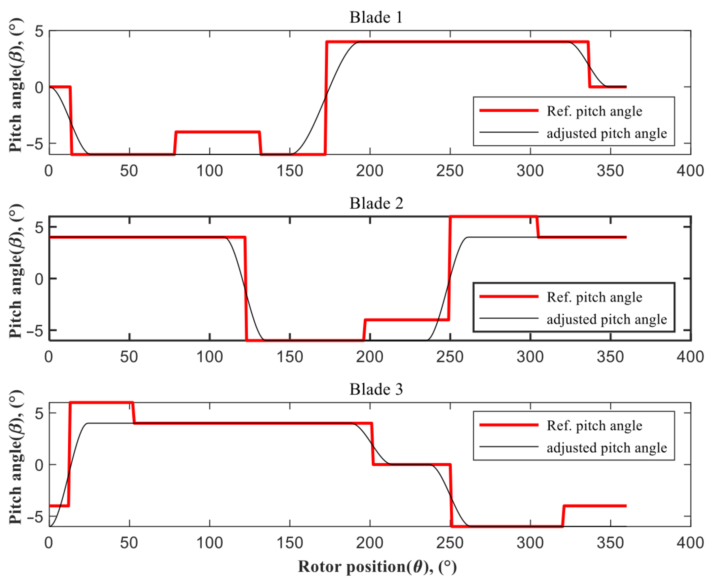
5.2. Pitch Angle Control System Effectiveness

While conducting the indoor tests, the pulley system was not attached. Therefore, the hybrid pitch control system was extensively tested indoors by using different user-specified percentages of the PID and MLP-ANN output signals.
For each blade, the response of the hybrid controller for three revolutions at different RPMs is compared to the reference pitch angles, as shown in Figure 13. Although the ability of obtaining a good set point tracking performance with the hybrid controller is challenging because of the small change in pitch angles, it can be seen that using a large percentage of a PID output signal (80%) resulted in a reasonable pitch angle response for only low RPMs. Overshoots are observed at the higher RPMs. However, the nonlinear dynamics of the H-type VAWT is evident at the higher RPMs. The control of these dynamics is improved by using a large percentage of the MLP-ANN output signal (i.e., 80 % MLP-ANN) in order to achieve a desirable blade pitch control performance.
The differences between the reference pitch signal and the measured pitch signal are determined by calculating the root mean square error (RMSE). At high RPMs, RMSEs in Table 2 show that the hybrid controller that uses 80% of the MLP-ANN output signal has a good ability to track the set point in comparison to the hybrid controller that uses 80% of the PID output signals for all blades. However, the hybrid controller that uses 80% of the PID output signals can reasonably minimize the errors at low RPMs. Furthermore, lower RMSEs of the hybrid controller can be demonstrated for the second blade, which can be attributed to the simple shape of the reference signal for this blade compared to the first and third blades.
For one rotor revolution, the green and yellow areas shown in Figure 13 represent the upstream and downstream regions for the rotor, respectively. These regions are used to investigate the effectiveness of the pitch control system. This can be accomplished by determining the peak of the pitch control response for all blades. In general, it can be seen that the overshoot occurs in the downstream region for the first and second blades. For the third blade, the overshoot only occurs in the upstream region for the first revolution, in contrast to the downstream region, where the overshoot is seen to occur in the second and third revolutions.
In fact, the downstream region is subject to the aerodynamic influence of the vortex shedding that is produced from the upstream blade. This may be the cause of the overshoot by the hybrid controller in the downstream region. The percentage overshoot (PO) of the hybrid controller response in the downstream region is summarized in Table 3. For all blades, POs for the hybrid controller that uses 80% MLP-ANN at high RPMs are less than those for the other two controllers that use 80% of PID output signals at both low and high RPMs.
Although the derivative parameter k D of the PID controller has been added (Table 1) in order to decrease the overshoot by the hybrid controller, it is seen that the controller that uses 80 % of the PID output signal had a limited ability to reduce the overshoot at high RPMs. The percentage decrease is calculated between the POs for both cases of the hybrid controller at high RPMs (i.e., 80 % PID and 80 % MLP-ANN), and the results showed that the hybrid controller that uses 80 % MLP-ANN is able to reduce the overshoot by 20 % , 15.901 % , and 15 % for each blade in comparison to the controller that uses 80 % of the PID command.
The POs for the first blade are generally lower than those in the second and third blades, owing to the fact that the gains of the PID controller for the first blade are greater than those for the other two blades, as shown in Table 1.
The proposed hybrid controller needs more enhancement. However, the results showed that this controller provided a significant improvement in terms of the power output from the H-type VAWT, with a small change in the pitch angles. Finally, the controller presented a good response at high RPMs, a regime of turbine operation that is associated with significant nonlinear dynamics.

6. Conclusions

The proposed hybrid controller, which consists of a nonlinear controller based on a neural network (MLP-ANN) and a conventional PID controller, has been developed for controlling the pitch angle of each blade of a Darrieus H-type VAWT individually. To investigate the stability of the proposed controller, a stability analysis is conducted using Lyapunov theory. For validation purposes, an H-type VAWT prototype is built, including the proposed controller implementation. The self-starting capability was improved by using the blade pitching technique. The results also reveal that, compared to the fixed pitch angle operation, the blade pitch control system clearly increases the power output of the H-type VAWT, with a percentage improvement that exceeded 22%. Finally, the hybrid controller that uses a high percentage of the MLP-ANN command is able to reduce the overshoot of the setpoint value at high rotor RPMs.

Author Contributions

Conceptualization, G.A., F.-S.L. and W.W.M.; methodology, G.A.; software, G.A. and M.A.D.; validation, G.A. and M.A.D.; formal analysis, G.A.; investigation, G.A.; resources, W.W.M.; data analysis, G.A. and M.A.D.; writing—original draft preparation, G.A.; writing—review and editing, F.-S.L., W.W.M. and E.Y.; supervision, F.-S.L., W.W.M. and E.Y. All authors have read and agreed to the published version of the manuscript.

Funding

This research received no external funding.

Institutional Review Board Statement

Not applicable.

Informed Consent Statement

Not applicable.

Data Availability Statement

The data presented in this study are available from the corresponding author on request.

Acknowledgments

The authors thank the financial support of the Libyan Ministry of Higher Education.

Conflicts of Interest

The authors declare no conflict of interest.

References

  1. Würfel, P.; Würfel, U. Physics of Solar Cells: From Basic Principles to Advanced Concepts; John Wiley & Sons: Hoboken, NJ, USA, 2016. [Google Scholar]
  2. Howell, R.; Qin, N.; Edwards, J.; Durrani, N. Wind tunnel and numerical study of a small vertical axis wind turbine. Renew. Energy 2010, 35, 412–422. [Google Scholar] [CrossRef] [Green Version]
  3. Chen, Y. Numerical Simulation of the Aerodynamic Performance of an H-Rotor. Master’s Thesis, University of Louisville, Louisville, KY, USA, 2011. [Google Scholar]
  4. Carrigan, T.J.; Dennis, B.H.; Han, Z.X.; Wang, B.P. Aerodynamic shape optimization of a vertical-axis wind turbine using differential evolution. ISRN Renew. Energy 2012, 2012, 528418. [Google Scholar] [CrossRef] [Green Version]
  5. Dyachuk, E.; Rossander, M.; Goude, A.; Bernhoff, H. Measurements of the aerodynamic normal forces on a 12-kW straight-bladed vertical axis wind turbine. Energies 2015, 8, 8482–8496. [Google Scholar] [CrossRef] [Green Version]
  6. Bos, R. Self-Starting of a Small Urban Darrieus Rotor—Strategies to Boost Performance in Low-Reynolds-Number Flows. Master’s Thesis, Delft University of Technology, Delft, The Netherlands, 2012. [Google Scholar]
  7. Khalid, S.S.; Liang, Z.; Qi-Hu, S.; Xue-Wei, Z. Difference between fixed and variable pitch vertical axis tidal turbine-using CFD analysis in CFX. Res. J. Appl. Sci. Eng. Technol. 2013, 1, 319–325. [Google Scholar]
  8. Jain, P.; Abhishek, A. Performance prediction and fundamental understanding of small scale vertical axis wind turbine with variable amplitude blade pitching. Renew. Energy 2016, 97, 97–113. [Google Scholar] [CrossRef]
  9. Lazauskas, L. Three pitch control systems for vertical axis wind turbines compared. Wind. Eng. 1992, 16, 269–282. [Google Scholar]
  10. Kirke, B.K. Evaluation of Self-Starting Vertical Axis Wind Turbines for Stand-Alone Applications. Ph.D. Thesis, Griffith University Gold Coast, Meadowbrook, QLD, Australia, 1998. [Google Scholar]
  11. Baker, J. Features to aid or enable self starting of fixed pitch low solidity vertical axis wind turbines. J. Wind. Eng. Ind. Aerodyn. 1983, 15, 369–380. [Google Scholar] [CrossRef]
  12. Hill, N.; Dominy, R.; Ingram, G.; Dominy, J. Darrieus turbines: The physics of self-starting. Proc. Inst. Mech. Eng. Part J. Power Energy 2009, 223, 21–29. [Google Scholar] [CrossRef]
  13. Ebert, P.; Wood, D. Observations of the starting behaviour of a small horizontalaxis wind turbine. Renew. Energy 1997, 12, 245–257. [Google Scholar] [CrossRef]
  14. Li, C.; Zhu, S.; Xu, Y.l.; Xiao, Y. 2.5 D large eddy simulation of vertical axis wind turbine in consideration of high angle of attack flow. Renew. Energy 2013, 51, 317–330. [Google Scholar] [CrossRef] [Green Version]
  15. Van, T.L.; Nguyen, T.H.; Lee, D.C. Advanced pitch angle control based on fuzzy logic for variable-speed wind turbine systems. IEEE Trans. Energy Convers. 2015, 30, 578–587. [Google Scholar] [CrossRef]
  16. Lee, S.H.; Joo, Y.J.; Back, J.; Seo, J.H. Sliding mode controller for torque and pitch control of wind power system based on PMSG. In Proceedings of the ICCAS 2010, Gyeonggi-do, Korea, 27–30 October 2010; pp. 1079–1084. [Google Scholar]
  17. Kasabov, N.K. Foundations of Neural Networks, Fuzzy Systems, and Knowledge Engineering; MIT Press: Cambridge, MA, USA, 1996. [Google Scholar]
  18. Tiwari, R.; Babu, N.R. Comparative Analysis of Pitch Angle Controller Strategies for PMSG Based Wind Energy Conversion System. Int. J. Intell. Syst. Appl. 2017, 9, 62–73. [Google Scholar] [CrossRef] [Green Version]
  19. Sargolzaei, J. Prediction of the power ratio and torque in wind turbine Savonius rotors using artificial neural networks. In Proceedings of the WSEAS International Conference on Renewable Energy Sources, Arcachon, France, 14–16 October 2007; pp. 14–16. [Google Scholar]
  20. Hossain, A.; Rahman, A.; Rahman, M.; Hasan, S.; Hossen, J. Prediction of power generation of small scale vertical axis wind turbine using fuzzy logic. J. Urban Environ. Eng. 2009, 3, 43–51. [Google Scholar] [CrossRef]
  21. Lee, M.J.; Hwang, G.H.; Jang, W.T.; Cha, K.H. Robotic agent control based on adaptive intelligent algorithm in ubiquitous networks. In KES International Symposium on Agent and Multi-Agent Systems: Technologies and Applications; Springer: Berlin/Heidelberg, Germany, 2007; pp. 539–548. [Google Scholar]
  22. Pezeshki, S.; Badalkhani, S.; Javadi, A. Performance Analysis of a Neuro-PID Controller Applied to a Robot Manipulator. Int. J. Adv. Robot. Syst. 2012, 9, 163. [Google Scholar] [CrossRef]
  23. Abdalrahman, G.; Melek, W.; Lien, F.S. Pitch angle control for a small-scale Darrieus vertical axis wind turbine with straight blades (H-Type VAWT). Renew. Energy 2017, 114, 1353–1362. [Google Scholar] [CrossRef] [Green Version]
  24. Semrau, G. Dynamic Modeling and Characterization of a Wind Turbine System Leading to Controls Development. Master’s Thesis, Rochester Institute of Technology, Rochester, NY, USA, 2010. [Google Scholar]
  25. Thomsen, S.C. Nonlinear Control of a Wind Turbine. Master’s Thesis, Technical University of Denmark, Lyngby, Denmark, 2006. [Google Scholar]
  26. Semrau, G.; Rimkus, S.; Das, T. Nonlinear systems analysis and control of variable speed wind turbines for multiregime operation. J. Dyn. Syst. Meas. Control 2015, 137, 041007. [Google Scholar] [CrossRef]
  27. Johnson, K.E.; Pao, L.Y.; Balas, M.J.; Fingersh, L.J. Control of variable-speed wind turbines: Standard and adaptive techniques for maximizing energy capture. IEEE Control Syst. Mag. 2006, 26, 70–81. [Google Scholar]
  28. Khan, S.A.; Rajkumar, R.K.; Rajkumar, R.K.; Aravind, C.V. Performance analysis of 20 pole 1.5 kW three phase permanent magnet synchronous generator for low speed vertical axis wind turbine. Energy Power Eng. 2013, 5, 423–428. [Google Scholar] [CrossRef]
  29. Muhando, E.B.; Senjyu, T.; Uehara, A.; Funabashi, T.; Kim, C.H. LQG design for megawatt-class WECS with DFIG based on functional models’ fidelity prerequisites. IEEE Trans. Energy Convers. 2009, 24, 893–904. [Google Scholar] [CrossRef]
  30. Jiao, X.; Meng, W.; Yang, Q.; Fu, L.; Chen, Q. Adaptive Continuous Neural Pitch Angle Control for Variable-Speed Wind Turbines. Asian J. Control. 2019, 21, 1–14. [Google Scholar] [CrossRef]
  31. Khalil, H. Nonlinear System; Wiley: Hoboken, NJ, USA, 1992. [Google Scholar]
  32. Nikravesh, S.K.Y. Nonlinear Systems Stability Analysis: Lyapunov-Based Approach; CRC Press: Boca Raton, FL, USA, 2016. [Google Scholar]
  33. Murray, R.M. A Mathematical Introduction to Robotic Manipulation; CRC Press: Boca Raton, FL, USA, 2017. [Google Scholar]
  34. Sapna, S.; Tamilarasi, A.; Kumar, M.P. Backpropagation learning algorithm based on Levenberg Marquardt algorithm. Comp. Sci. Inform. Technol. 2012, 2, 393–398. [Google Scholar]
Figure 1. Forces and velocities acting on the blade of a Darrieus turbine.
Energies 15 00235 g001
Figure 2. Main components of an H-type VAWT model.
Energies 15 00235 g002
Figure 3. Wind turbine drive-train model based on a two-mass model.
Energies 15 00235 g003
Figure 4. C p λ curve and equilibrium points of a wind turbine.
Energies 15 00235 g004
Figure 5. Equilibrium points for a variable pitch angle wind turbine [26].
Energies 15 00235 g005
Figure 6. Final assembly of the H-type VAWT.
Energies 15 00235 g006
Figure 7. Blade pitch control system and data logging.
Energies 15 00235 g007
Figure 8. A block diagram of the blade pitch control system for one blade.
Energies 15 00235 g008
Figure 9. Original and adjusted reference pitch angles.
Energies 15 00235 g009
Figure 10. Pitch control system experimental setup.
Energies 15 00235 g010
Figure 11. H-type VAWT power generation for the first test: (a) fixed pitch angle (b) variable pitch angle.
Energies 15 00235 g011
Figure 12. Filtered power generation curves for the first test, and in both fixed and variable pitch angle configurations.
Energies 15 00235 g012
Figure 13. Response of hybrid controller for (a) blade 1, (b) blade 2 and (c) blade 3 at different RPMs.
Energies 15 00235 g013
Table 1. PID gains for each blade.
k P k I k D
Blade 10.121000.043
Blade 20.0881000.009
Blade 30.11000.01
Table 2. RMSE of hybrid controller for different weights.
RMSE80% PID and 20%
MLP-ANN at
Low RPM
80% PID and 20%
MLP-ANN at
High RPM
80% MLP-ANN
and 20% PID at
High RPM
Blade 13.21813.27411.7961
Blade 21.66292.87321.8962
Blade 32.62483.02382.4718
Table 3. Percentage overshoot of the hybrid controller for the first revolution.
PO
(Ref.)
Pitch = 10
80% PID and 20%
MLP-ANN at
Low RPM, (%)
80% PID and 20%
MLP-ANN at
High RPM, (%)
80% MLP-ANN
and 20% PID at
High RPM, (%)
Blade 110.4271.7
Blade 22531.511.7
Blade 313.3289
Publisher’s Note: MDPI stays neutral with regard to jurisdictional claims in published maps and institutional affiliations.

