Modelling and Environmental Assessment of a Stand-Alone Micro-Grid System in a Mountain Hut Using Renewables

Abstract

Mountain huts are stand-alone micro-grid systems that are not connected to a power grid. However, they impact the environment by generating electricity and through day-to-day operations. The installed generator needs to be flexible to cover fluctuations in the energy demand. Replacing fossil fuels with renewable energy sources presents a challenge when it comes to balancing electricity generation and consumption. This paper presents an integration-and-optimization process for renewable energy sources in a mountain hut’s electricity generation system combined with a lifecycle assessment. A custom computational model was developed, validated with experimental data and integrated into a TRNSYS model. Five different electricity generation topologies were modelled to find the best configuration that matches the dynamics and meets the cumulative electricity demand. A lifecycle assessment methodology was used to evaluate the environmental impacts of all the topologies for one typical operating year. The carbon footprint could be reduced by 34% in the case of the actually implemented system upgrade, and by up to 47% in the case of 100% renewable electricity generation. An investment cost analysis shows that improving the battery charging strategy has a minor effect on the payback time, but it can significantly reduce the environmental impacts.

1. Introduction

Stand-alone micro-grid systems have been widely studied, discussed, demonstrated and even tested in residential applications, but they are rarely discussed and applied to mountain huts (MHs). MHs have a specific energy demand that provides suitable living and working conditions for the staff as well as comfort for the visitors [1]. To generate sufficient electrical energy throughout the days, weeks, months and years, MH micro-grid systems in the past relied mostly on fossil-fuel-based technologies that are easy to operate are affordable [2,3], but these are far from optimal when considering the environmental impacts and target emissions such as NOx or particles [4,5]. Nowadays, the environmental approach is a top priority in natural environments, where pollution is a critical factor and different authorities look for the best measures to prevent the deterioration and contamination of natural habitats with wild fauna and flora [6,7]. EU policy is for a more sustainable and low-carbon economy and the example of an MH is a perfect demonstration of the highly efficient penetration of local renewable energy sources, which is among the many targets of the European Commission’s sustainable approach [8,9]. Besides technical feasibility and environmental impacts, the economic aspects of energy systems should also be considered. Mori et al. [10] show that the optimal system might not be the best one considering any single criterion, but should instead be a reasonable balance among energy efficiency, environmental impacts and economic constraints.

Fully energy-self-sufficient buildings are still very rare, but the integration of photovoltaics (PV), wind power and small energy storage systems has become popular in residential areas [11,12]. PVs were shown to be a potential route with which to achieve a zero-emissions building or even a positive-energy building by Zomer et al. [13]. The integration of renewable energy sources (RESs) into an energy supply system raises certain issues when it comes to balancing electricity demand and supply because of their variable and non-storable nature [14]. This applies to wind energy and PVs, which are two technologies that could be effectively implemented in MHs throughout Europe [15]. Stand-alone systems represent a challenging case for RESs integration, due to the inability to import deficits and export surpluses of energy. Therefore, stand-alone energy systems require energy storage systems [16]. In the case of MHs, the storage can be a battery rack, a hydrogen storage system or a combination of both, depending on the micro-grid’s configuration and the availability of RESs. Lacko et al. presented the case of an isolated household in a coastal region using a hydrogen storage system [17,18]. Bojic et al. even used the grid as a virtual energy storage system [19]. Mulleriyawage et al. optimized their battery storage capacity for a PV–battery system in a household case study connected to the grid [20]. Apart from this, it was shown to be very challenging to achieve complete independence from the grid in many cases [21].

In addition, in MHs, all the technologies are subjected to much greater challenges due to the specific operational dynamics and the extreme weather conditions. Research in Antarctica with a hydrogen storage system linked to PVs in extreme weather conditions was discussed by Cabezas et al. [22], and the combination of wind power and an alkaline electrolyser in Norway was considered by Ulleberg et al. [23]. One of the limitations of the studies with stand-alone MH energy systems based on RESs is the lack of required input data, such as the local metrological conditions (wind, sun, temperature, humidity) and exact MH electrical load profiles (peak power, cumulative energy requirements, daily dynamics) that define the nominal power of the installed RES system and the capacity of the energy storage system [24]. To optimize the operation and make micro-grid systems sufficient in all conditions, the focus of the research should be on power and energy management [25,26]. Ayeng’o et al. presented a PV model for determining the optimal configuration point between PVs and batteries using many parameters that influence the output voltage [27]. Cho et al. showed that the proper sizing of the batteries is critical for the better operation of a stand-alone system [28]. Soudan et al. studied three scenarios for optimizing a PV–battery–diesel off-grid installation by considering different operational conditions (cloudiness, time of irradiation, etc.) [29]. By adding the economic criteria of Haratian et al. in an off-grid renewable energy system, including a solar panel, a wind turbine and batteries, it was shown that the most economical configuration among different RES configurations was the PV–battery combination [30].

An MH that is in a sensitive natural habitat has negative environmental impacts because of its operation. Environmental impacts during the year arise due to different direct (electricity generation, heat generation, wastes from operation, septic tank, etc.) and indirect activities (transport, wastes from visitors, etc.) that cause emissions into the air, water and soil, and have an impact on the Earth’s resources [31]. Focusing on energy generation, most environmental impacts arise from electricity and heat, if the energy is generated from fossil fuels such as diesel, gasoline, liquefied petroleum gas and natural gas [32]. With the integration of RESs, the environmental impacts could be significantly reduced due to a reduction in the use of fossil fuels, but energy storage systems have to be properly introduced and optimized, depending on the availability of the RESs and the MH’s energy demands [33]. It was shown by Mori et al. that 1 kWh of electricity generated from small gen-sets has a carbon footprint of approximately 920 g CO₂ eq./kWh, compared to the carbon footprint of micro-hydro with just 4 g CO₂ eq./kWh, micro-wind with 40 g CO₂ eq./kWh or PVs on a slanted roof with 220 g of CO₂ eq./kWh [1]. However, we must be aware that the carbon footprint is a global indicator, and, in natural habitats, more indicators have to be observed since environmental impacts on local and regional scales are of great importance.

This paper presents a techno–environmental–economic approach to an electricity generation system’s optimization. There are many techno–economic studies of stand-alone energy systems available, but these are without environmental impact assessments, which are becoming one of the most important decision criteria. The study was conducted based on local RESs’ availability, an installed electricity generation system, current control protocols and an MH load profile based on 1 year of measured operational data. A custom computational model for a load assessment was developed and further integrated into a TRNSYS energy system model. Prior to the integration, the computational model was verified using experimental data. Additional electricity generation scenarios were defined to reach the highest possible renewables penetration and try to lower the environmental impacts. To obtain the optimal system topology, the technical, environmental and economic (investment costs) parameters are discussed. With this approach, the decision criteria are taken to a higher level, including the environmental profile as a very important factor.

An introduction to the current energy system’s topology in the MH and its micro-grid are presented in Section 2, where the simulated scenarios are also described. Section 3 presents the available system operation data, the custom computational model development and the pre-processing of the input data. The results are presented and discussed in Section 4, while Section 5 addresses the environmental assessment and environmental impacts. The paper ends with a discussion of the results in Section 6, and the main conclusions are drawn in Section 7.

2. Micro-Grid System and Definition of the Simulated Scenarios

The Refugio de Lizara MH is in a natural park of the Spanish Pyrenees at an elevation of 1540 m. It has a capacity of 78 people and free access to electricity, hot water and other services [34]. The largest share of the electricity needed for the MH’s operation is generated by two diesel generators (gen-sets) of 22.4 and 12.8 kWe that are used daily during peak demands (breakfast, lunch and dinner) and a PV system with a nominal power of 3.7 kWp. The energy system was recently modified and upgraded to make it more sustainable and environmentally sounder. The installation of additional PVs, a control system and waste heat recuperation was made as part of the LIFE SustainHuts project [31]. The increase in the installed PV power from 0.5 kWp in the state of play at the beginning (SOBP) to 3.7 kWp in the state of play at the end (SOPE) was realized to increase the RES penetration and lower the environmental impacts. With no automated control system for the micro-grid in the SOPB, manual control was required, which introduced errors into the energy management and caused lower efficiency of the system, resulting in more operating hours for the gen-sets and increased fuel consumption. The surplus electricity (from the gen-sets or PVs) is stored in a lead–acid battery pack with a total capacity of 38.4 kWh, which provides the electricity when the gen-sets or PVs are not in operation. Heat is generated with a propane gas heater of 30 kW coupled to a boiler and a central heating system. A classic open chimney was used with the SOPB in the main room and mixed wood was used as a fuel. In the SOPE, waste heat recuperation from the flue gases was installed.

Table 1. State of play of the Lizara hut at the beginning (SOPB) and after modifications (SOPE).

	SOPB	SOPE
Diesel generator (kWp)	22.4 + 12.8	22.4 + 12.8
PV (kWp)	0.53	3.7
Batteries (kWh)	38.4	38.4
Chimney	Open chimney	Heat recuperation
Micro-grid control	Manual	Manual
Diesel (L/year)	5774	4511
LPG (kg/year)	6568	3140
Mixed wood (kg/year)	700	5000

presents the SOPB and SOPE with the technologies installed and the annual diesel consumption data for electricity generation and liquefied petroleum gas (LPG) and mixed wood consumption for the heat generation and the cooking. The annual consumption of fossil fuels changes, depending on the weather, the number of visitors and for other reasons. The annual average in previous years was just below 6000 L of diesel (for electricity generation) and around 6600 kg of propane (for heating and cooking). The mixed wood consumption was drastically increased from the SOPB (700 kg) to SOPE (5000 kg) because, in the SOPE, the water was heated with recuperated heat instead of with LPG as in the SOPB.

Figure 1 shows the basic scheme of the Lizara micro-grid for electricity generation. The consumers of electricity define the specific nature of the electricity generation system. The hut and all the devices connected to the base hut’s electricity system represent a single-phase load; auxiliary devices and machines, mostly used in the kitchen, represent a three-phase load and a separate grid. Since the three-phase loads cannot be avoided and are only used occasionally, the optimization process introduced in this study will focus on the single-phase load. Furthermore, typical electricity systems in MHs across Europe are only single-phase, so the workflow presented in this paper could be applied to other MHs.

A computational model approach was used with several different settings in the MH to compare the various system configurations and operating scenarios. As the measured data are available only for the SOPE, this was simulated first to validate the custom computational model and to find the appropriate settings. The measured data showed that the PV system provided approximately 2929 kWh of electrical energy, which is less than 800 kWh per installed kWp per year. Studies show that for the location of the Lizara hut, approximately 1400 kWh could be produced annually with each kWp of the installed PV system [35]. This led us to the conclusion that there is potential for the more optimized energy management of the system that could provide better utilization of solar energy and thus reduce the need for fossil fuels. Therefore, the same basic system configuration as in the SOPE was further optimized with respect to the strategy of gen-set operation and battery charging. Furthermore, to prove the benefits of the system upgrade, the SOPB was also simulated. Finally, two theoretical configurations were considered: one with a doubled capacity for the PV panels and batteries with respect to the SOPE, and the other with the capacities of the PV panels and batteries sufficiently increased to enable fully renewable operation, i.e., the gen-set would no longer be needed. All the simulated configurations are as follows:

(i)

MEAS: system configuration after the upgrade, PV 3.7 kWp, batteries 38.4 kWh, gen-sets 12.8 + 22.4 kW, measurement results of actual 1-year operation of the hut.

(ii)

SOPE: system configuration after the upgrade, same as measured, used for validation of the custom computational model.

(iii)

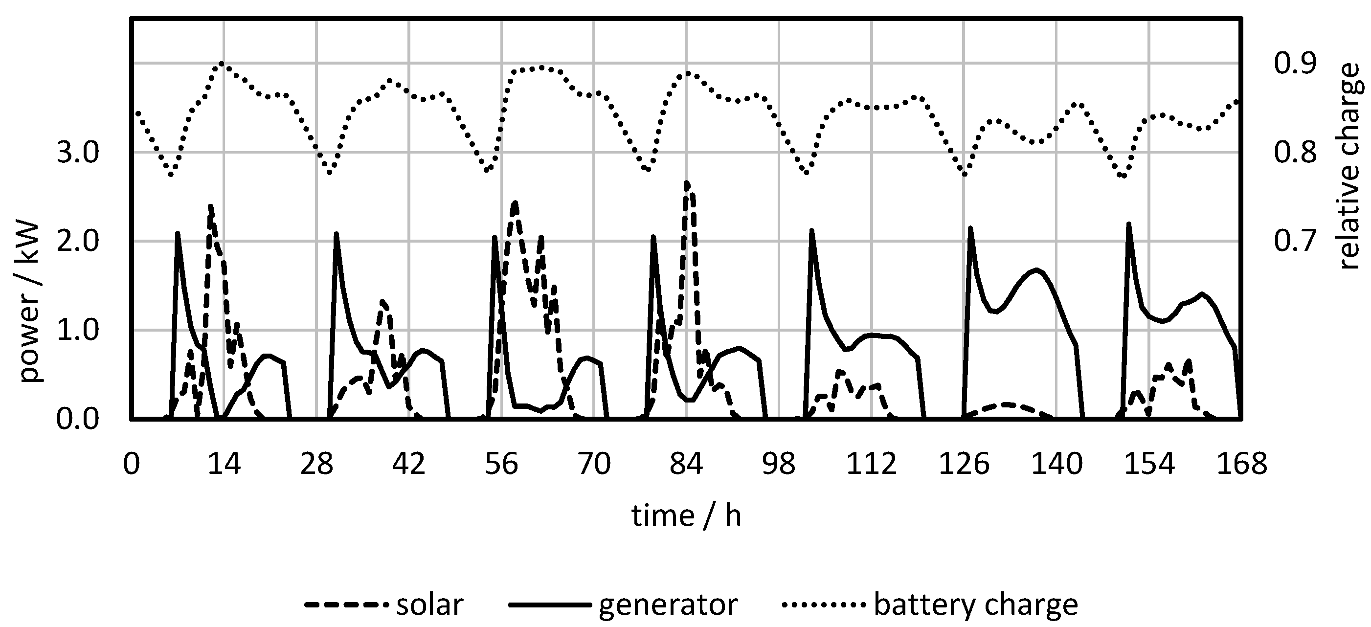
SOPE+: system configuration after the upgrade, same as the SOPE and measured but with modified battery charging strategy to increase the use of renewable energy.

(iv)

SOPB: system configuration before the upgrade for comparison with current state, PV 0.5 kWp, batteries 38.4 kWh, gen-sets 12.8 + 22.4 kW.

(v)

SOPEx2: hypothetical configuration with double PV and battery capacity compared to the SOPE; improved battery charging strategy was employed as in the SOPE+.

(vi)

RES: hypothetical configuration with sufficient PV and battery capacity for fully renewable operation; improved battery charging strategy was employed as in the SOPE+.

3. Computational Model and Input Data

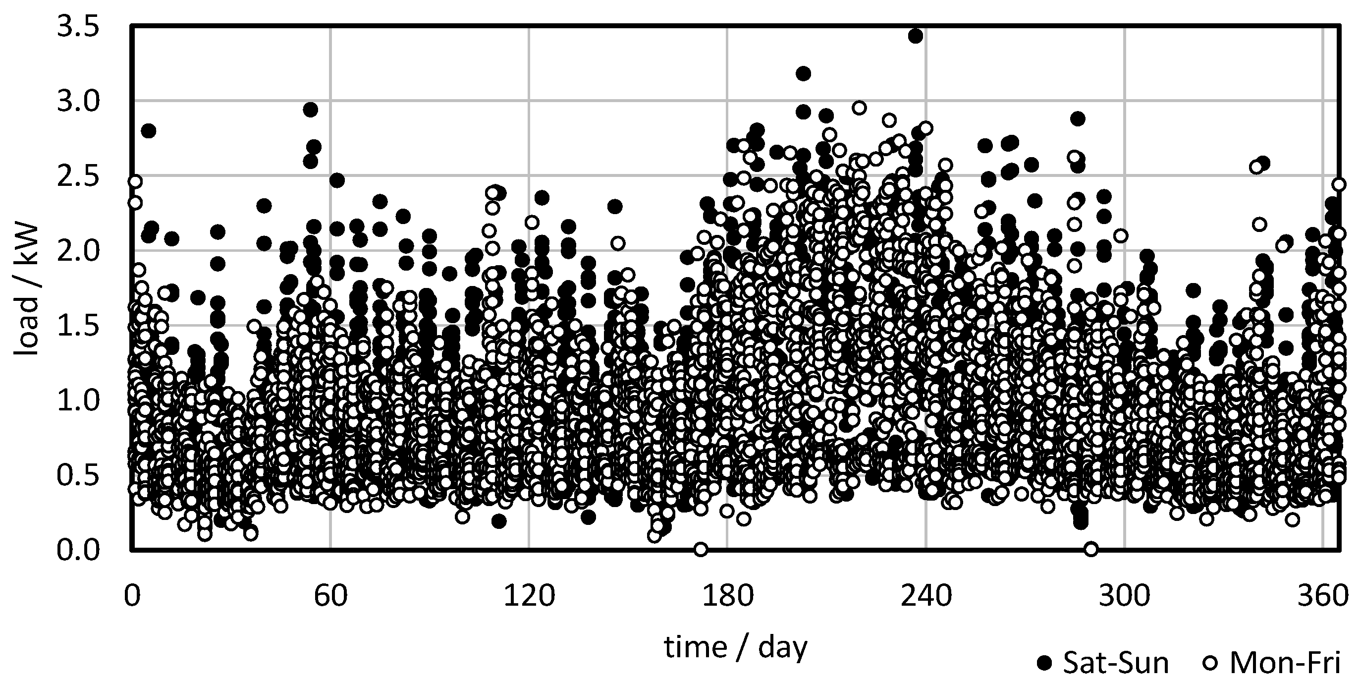
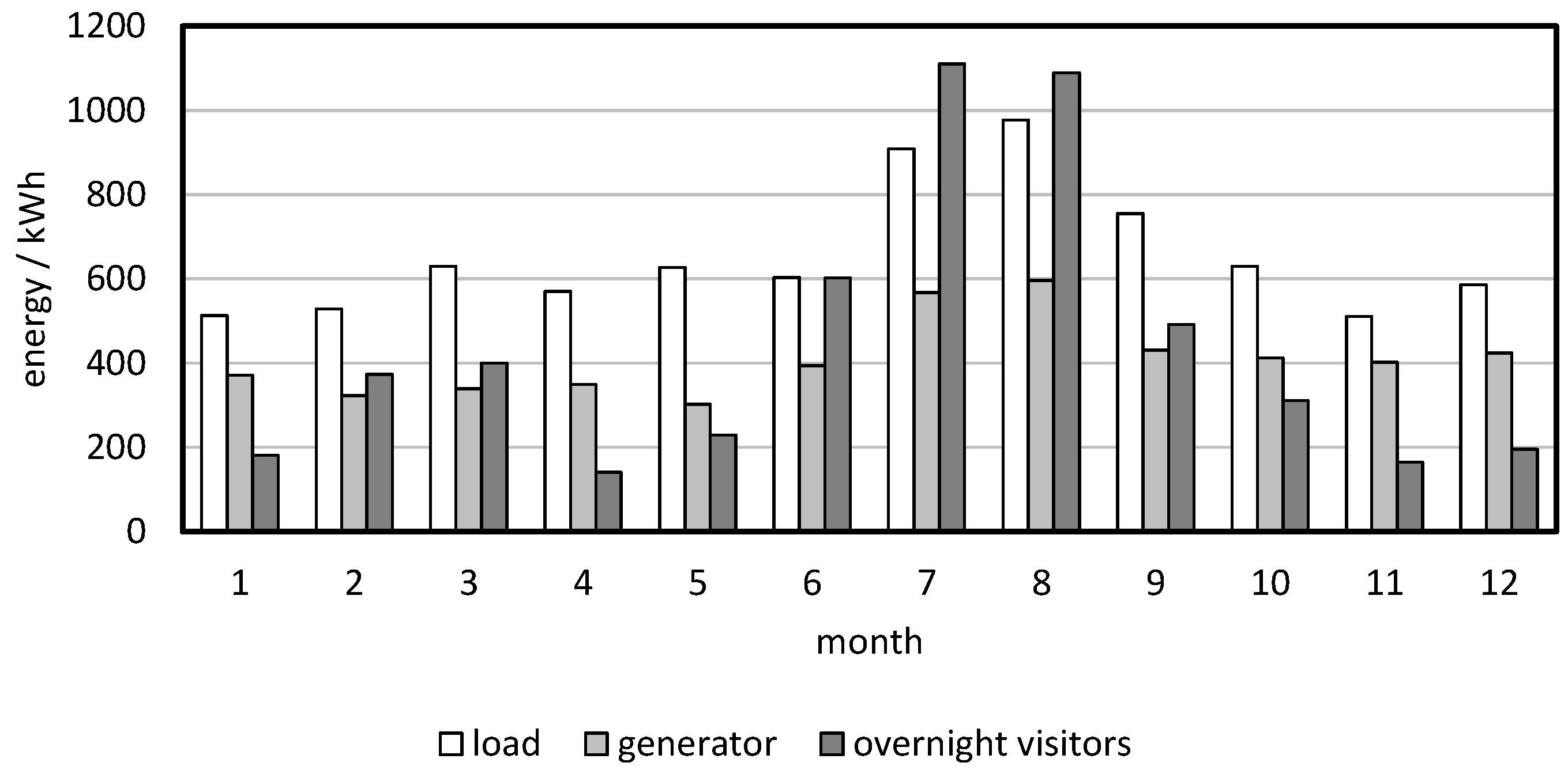
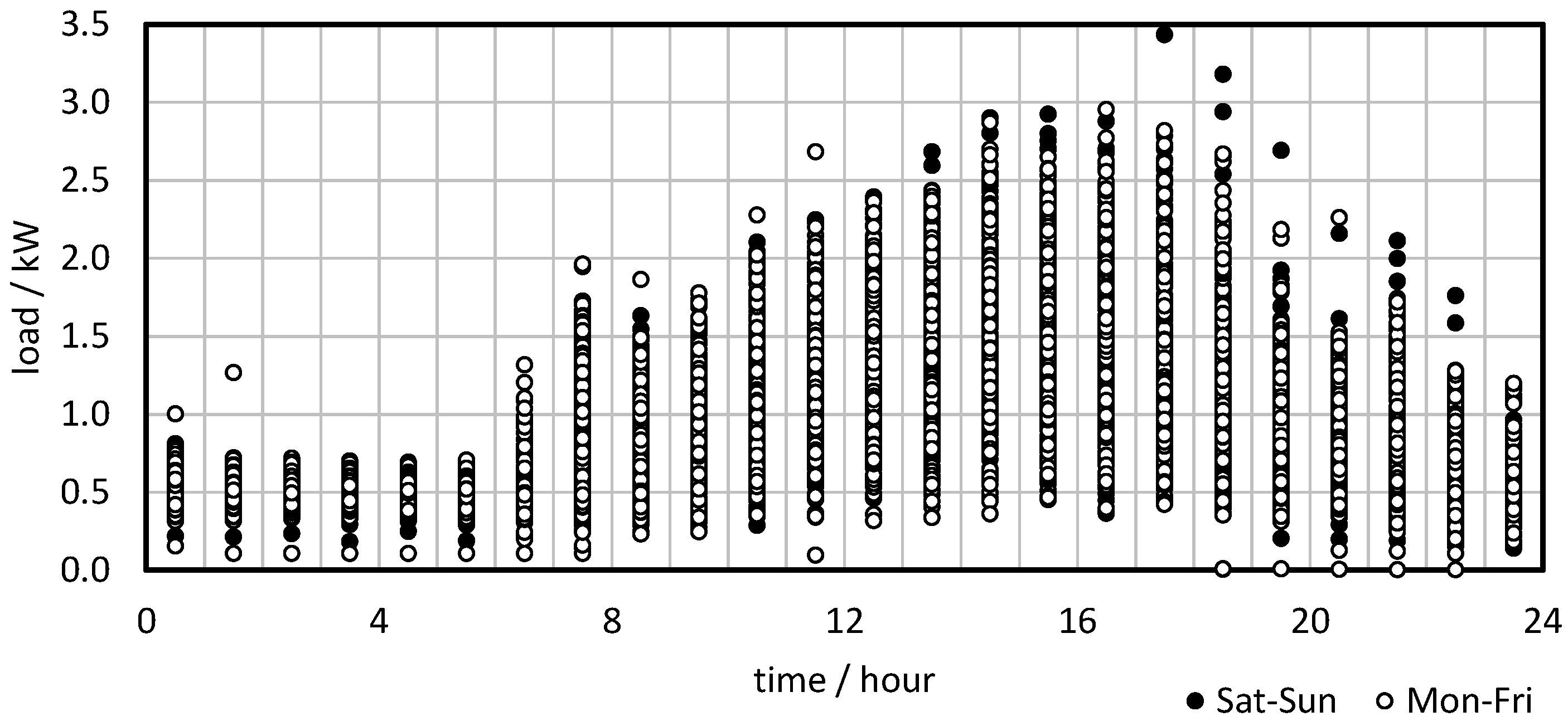
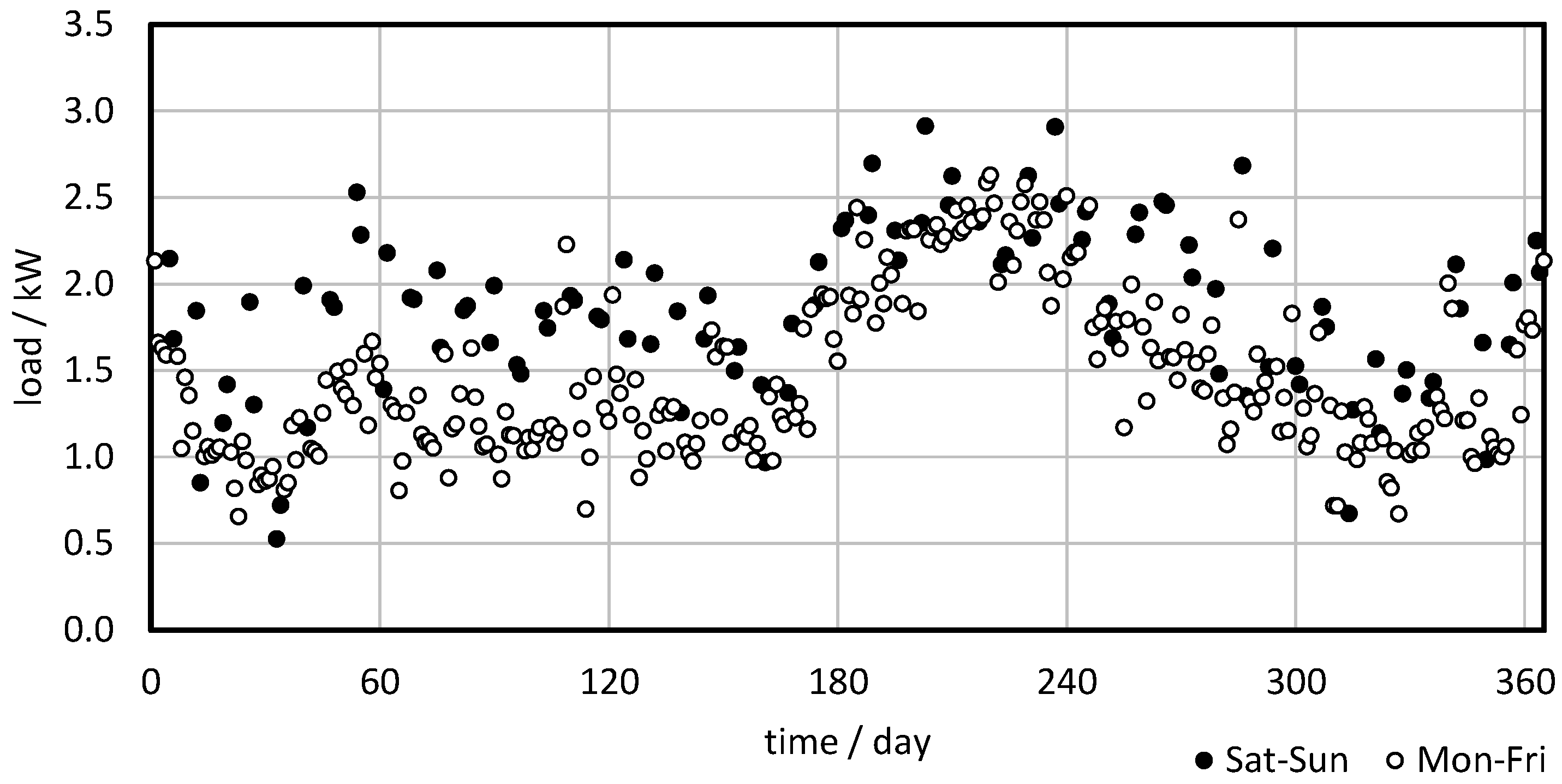
To analyze the performance and the environmental profile of the micro-grid system, the energy consumption (load) and the energy availability (renewable energy sources) data are required. Unfortunately, in the case of MHs, these data are usually not available. Therefore, it is necessary to develop appropriate models that describe both the load and the weather conditions with sufficient accuracy to enable further modelling of the entire system’s operation [36,37]. In this way, different system set-ups can be objectively compared using the same input data and the same approach.

3.1. Input Data

The input data for a non-stationary simulation of an energy system’s performance include the time series of both the generation and consumption sides of the system. To compare the performance and the environmental impacts of the different system set-ups, the generation-side and consumption-side data should be constant for all the observed configurations. Actual power consumption data are available with a resolution of 1 h, but the weather conditions or renewable resources are not known for the same period and at the observed location. The operation of the Lizara MH was monitored for 1 year from 1 June 2018 to 31 May 2019. Monthly integrals of the energy consumption and energy generation for the single-phase part of the system are presented in Figure 2. The difference between the measured values is assumed to be covered by the photovoltaic system, although the actual measured data are not available [38]. For comparison, the reported number of overnight visitors is also shown in Figure 2 to correlate the energy consumption with the number of visitors. Note that single-day visitors are not included in the presented data.

The consumption data were analyzed on two time scales: one showed the variation in the load over 365 days (Figure 3), while the other showed variations in the daily 24 h profile (Figure 4). Note that the yearly data were shifted so that day 1 represents 1 January. In both diagrams (Figure 3 and Figure 4), the days from Monday to Friday and weekends (Saturday and Sunday) are presented with different markers.

There are distinct periods with different loads, where the warmer part of the year has noticeably higher energy consumption than the rest of the year (Figure 3), with another notable peak around New Year. During the weekend (the black dots in Figure 3 and Figure 4), the load is higher than during the rest of the week, with the difference being more obvious during the colder part of the year. The energy consumption in a mountain hut is primarily related to the number of visitors, which is typically higher during the summer season, as well as during weekends and holidays. Therefore, a specific consumption profile needs to be developed that suits the operational characteristics of the mountain hut.

The night-time load is relatively constant from midnight to 6 AM and seasonal variations are therefore not expected, while the daytime load is more variable, and the magnitude is expected to be related to the seasons. A typical daily profile could be generated and scaled to match the seasonal variations.

$$W_{\mathrm{n}}\left(h,d\right)=\frac{W\left(h,d\right)-W_{\mathrm{base}}}{W_{\mathrm{high}}\left(d\right)-W_{\mathrm{base}}}$$

(1)

First, the daily profiles were normalized with the assumption that there is a constant base load throughout the year (average night-time load, W_base) and a daily peak that is unique for every day (W_high(d), d represents the number of days in a year). The daily peak consumptions were calculated as the average of the three highest loads of each day in order to avoid exceptionally high values. The normalized load (W_n(h,d), where h represents the hours in a day and d the days in a year) can be calculated from the measured load (W(h,d)), as presented in Equation (1).

The average normalized load as a daily profile is shown in Figure 5. Since the base load is subtracted for normalization, the values are around 0 during the night-time and increase towards 1 during the day. A simplified profile is also shown, which consists of five typical regions defined by the time of day.

$$W_{\mathrm{norm}}\left(t\right)=a_{\mathrm{norm},k}+b_{\mathrm{norm},k}\cdot t$$

(2)

The simplified, normalized load (W_norm(t)) is expressed as a set of linear functions with coefficients a_norm,k and b_norm,k, each covering a separate interval of the day, denoted by index k (Equation (2)).

To scale the normalized profile, the maximum loads throughout the year were analyzed (Figure 6), where the difference between the weekends and the rest of the week could be seen. Hence, separate rules are needed to properly describe this phenomenon (Figure 7).

The Monday–Friday and Saturday–Sunday profiles can be simplified with a similar approach to that used for the daily profiles in Equation (2).

$$W_{\mathrm{peak}}\left(d\right)=a_{\mathrm{peak},j}+b_{\mathrm{peak},j}\cdot d$$

(3)

Separate intervals (denoted with index j) are identified, where the linear relations between the daily peaks (W_peak(d)) and the serial number of the day (d) can be determined (Equation (3)). Different intervals and coefficients are used for Monday–Friday and Saturday–Sunday.

The described data analysis was performed with a custom-developed procedure and algorithms in MS Excel. To calculate the load for hour h of day d:

• It is necessary to know whether the particular day is a working day or a weekend day.
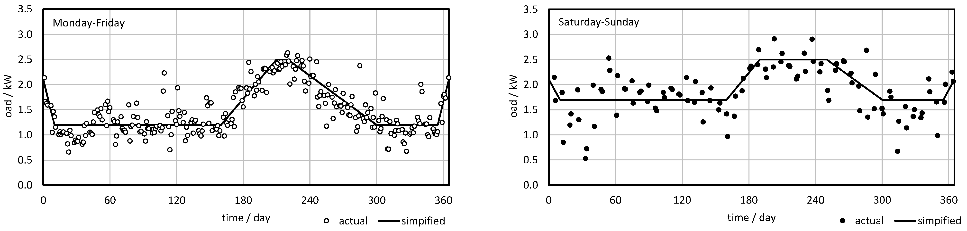
• It is necessary to know to which of the intervals j shown in Figure 7 the particular day belongs, so that appropriate coefficients a_peak,j and b_peak,j are selected.
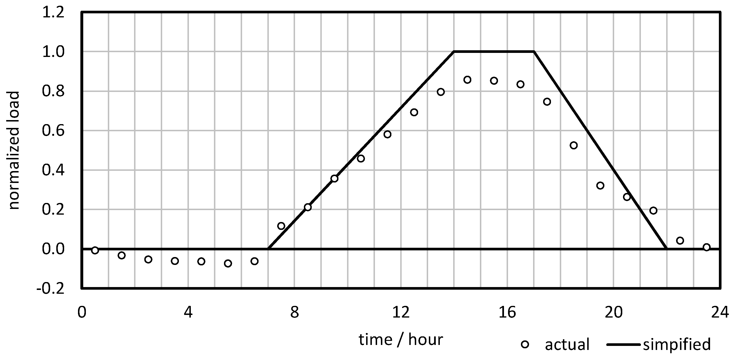
• It is necessary to know to which of the intervals k shown in Figure 5 the particular hour belongs, so that appropriate coefficients a_norm,k and b_norm,k are selected.
• Peak load of the day and normalized load of the hour are calculated according to Equations (2) and (3), respectively.
• Finally, the load is calculated as

$$W\left(h,d\right)=W_{\mathrm{base}}+W_{\mathrm{norm}}\left(h\right)\cdot W_{\mathrm{peak}}\left(d\right)$$

(4)

This way, a complete set of loads for all 8760 h of a year is calculated and compared with the measured year (Figure 8). Note that the use of weekend profiles depends on the actual day of the week that the observed year starts with, but it is not expected to have a significant influence on the integral parameters of the system’s performance. For a clearer comparison, both duration curves (modelled and measured) are presented in Figure 9. We can calculate that the average load and the standard deviation differ by only 3% and 1%, respectively.

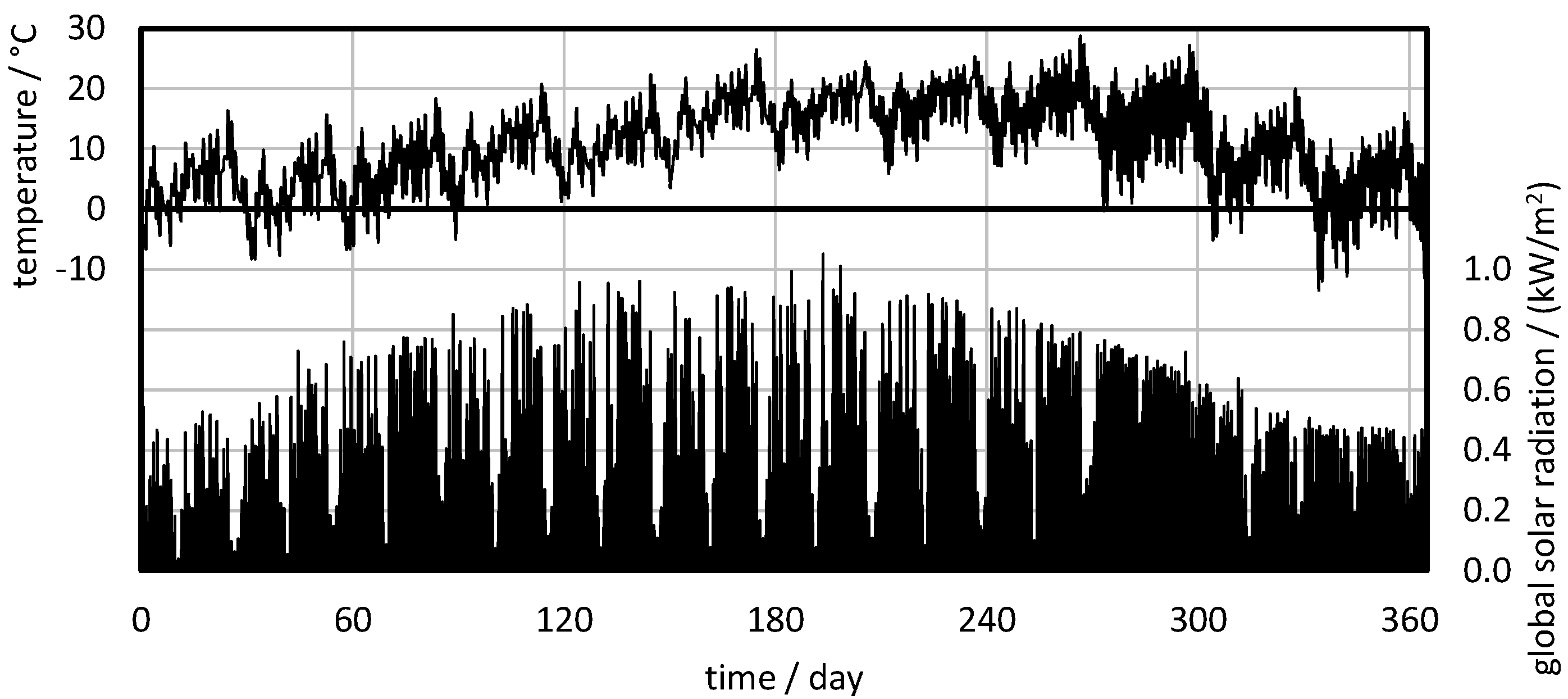
3.2. Weather Conditions

The production of electricity using RESs is dependent on the current local weather conditions, which can vary substantially with time and depend on the actual location. Detailed information is only known for a limited number of observation points. Therefore, appropriate interpolation and randomization models need to be used to model the representative weather conditions for the observed location throughout the simulated time frame. The weather simulation model that was used is based on algorithms developed by Knight et al. [39], Graham et al. [40], Degelman [41] and Gansler [42], and is a part of the TESS library used in the TRNSYS 17 simulation tool [43]. The model builds hourly profiles of the weather data based on monthly averages. These are acquired from www.renewables.ninja (accessed on 10 December 2021) [44] using the MERRA-2 model [45] with measured data from 2014 that were available at the time of the study. The generated weather data for the observed location are shown in Figure 10 and were used as a reference meteorological year for all the observed configurations. In this way, we ensured that the configurations were comparable, even though they were not built on actual measurements of the meteorological data at the exact location.

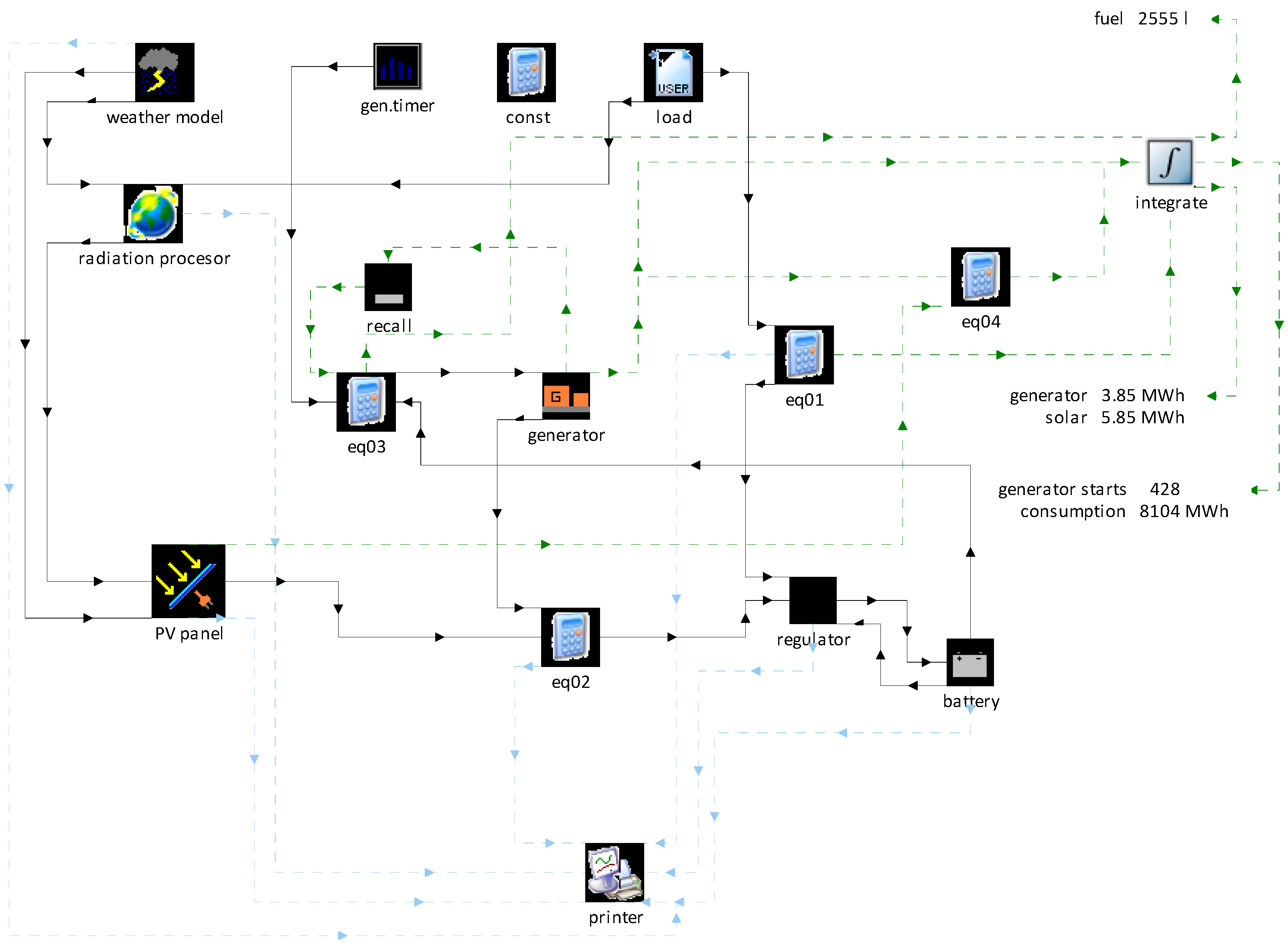
3.3. Energy System Model

The energy system of the MH was modelled with TRNSYS 17 software [46] using additional TESS libraries [43]. Since detailed and reliable performance data were not available for the specific components of the system, the most suitable generic models available in the software libraries were used. Previously introduced load and weather models were used as the input data and boundary conditions.

The complete model is presented in Figure 11 and consists of the following components: (i) inputs (weather data, load or power consumption and the generator’s operating schedule); (ii) power generation, storage and control (PV panels, gen-set, batteries and regulator), (iii) additional models (generator’s output control with respect to the current state of charge of the batteries and unit conversions) and (iv) outputs (data file with hourly values of selected performance data for further analyses and on-screen display of the integral operating parameters).

4. Energy Balance of the Modelled Configurations

The simulations produce time series of hourly data for numerous system performance parameters. Figure 12 shows the power being produced and the charge on the batteries for 1 week (168 h) for the SOPE. During the night, the charge on the batteries drops significantly as there is no electricity generation; however, the base load is always present.

During the day, the charge increases, but the increase is notably smaller on days with small insolation. The generator provides a higher output when the charge on the batteries is low and a lower output when solar power is available and the charge on the batteries is higher. The inputs for the simulations are modelled values of the load (Figure 8) and meteorological data (Figure 10). Therefore, it is not possible to compare the simulation results and the measured values on an hourly basis. On the other hand, it is possible to compare the integral values during longer periods (e.g., months). Figure 13 shows the notable similarity of the monthly generator outputs for the SOPE simulated (calculated) and the measured values.

We will only use selected integral parameters for further comparisons of the actual measured data and the different simulated configurations. The results are summarized in

Table 2. Comparison of the measured and calculated results for different configurations.

Description	Unit	SOPB	MEAS *	SOPE	SOPE+	SOPEx2	RES
total consumption	kWh	8105	7842	8105	8105	8105	8105
generator output	kWh	8284	4913	5064	3348	638	0
total fuel consumption, single phase	L	3408	2021	2083	1378	262	0
nominal photovoltaic power	kW	0.5	3.7	3.7	3.7	7.4	11.1
available solar energy	kWh	791	-	5852	5852	11,704	17,556
battery capacity	kWh	38.4	38.4	38.4	38.4	76.8	192.0
excess energy	kWh	0	-	1734	59	2996	7941
renewable penetration	%	8.7	-	44.9	63.4	93.2	100.0

* MEAS: represents the only configuration with real experimentally obtained data with the SOPE.

. The total consumption is all the electrical energy consumed by the MH in one year. The generator output represents the electrical energy provided by the gen-set for single-phase loads and the total fuel consumption is the quantity of diesel fuel for the generator attributed to the production of single-phase electricity. The available solar energy is the electrical energy that could be produced with photovoltaic panels if an appropriate load or free battery capacity is available. Due to the different dynamics of the load and the electricity generation, as well as the limited battery storage capacity, some of the available energy is not actually generated and so is labelled as excess energy. The renewables penetration is the fraction of produced solar energy in the total produced energy (solar and gen-set). Note that the total energy production exceeds the total consumption mainly due to energy loss during the charging and discharging of the batteries.

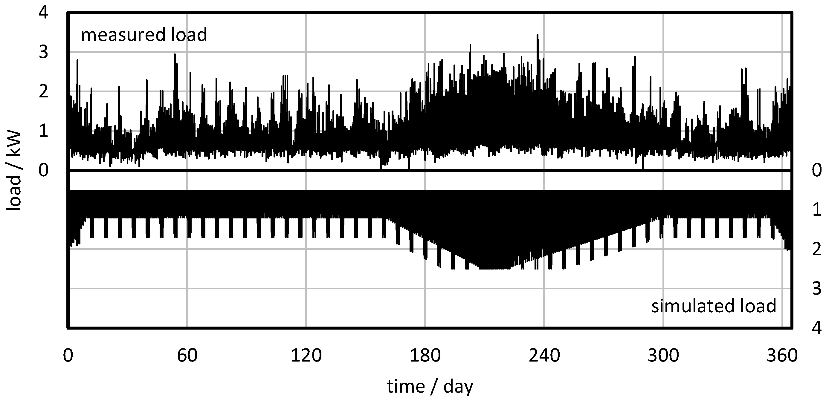
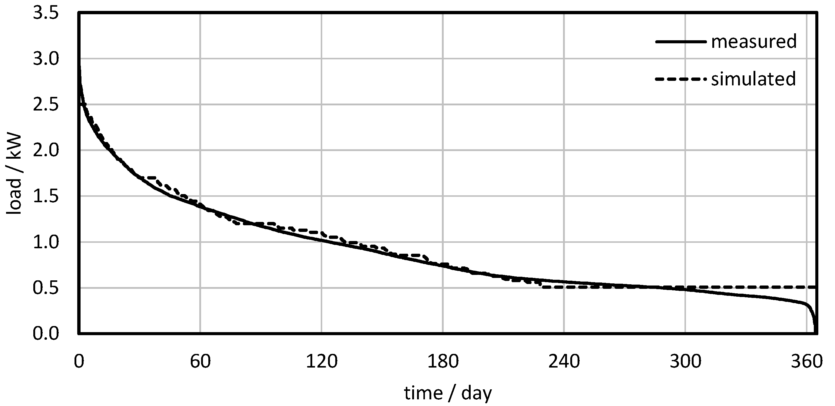
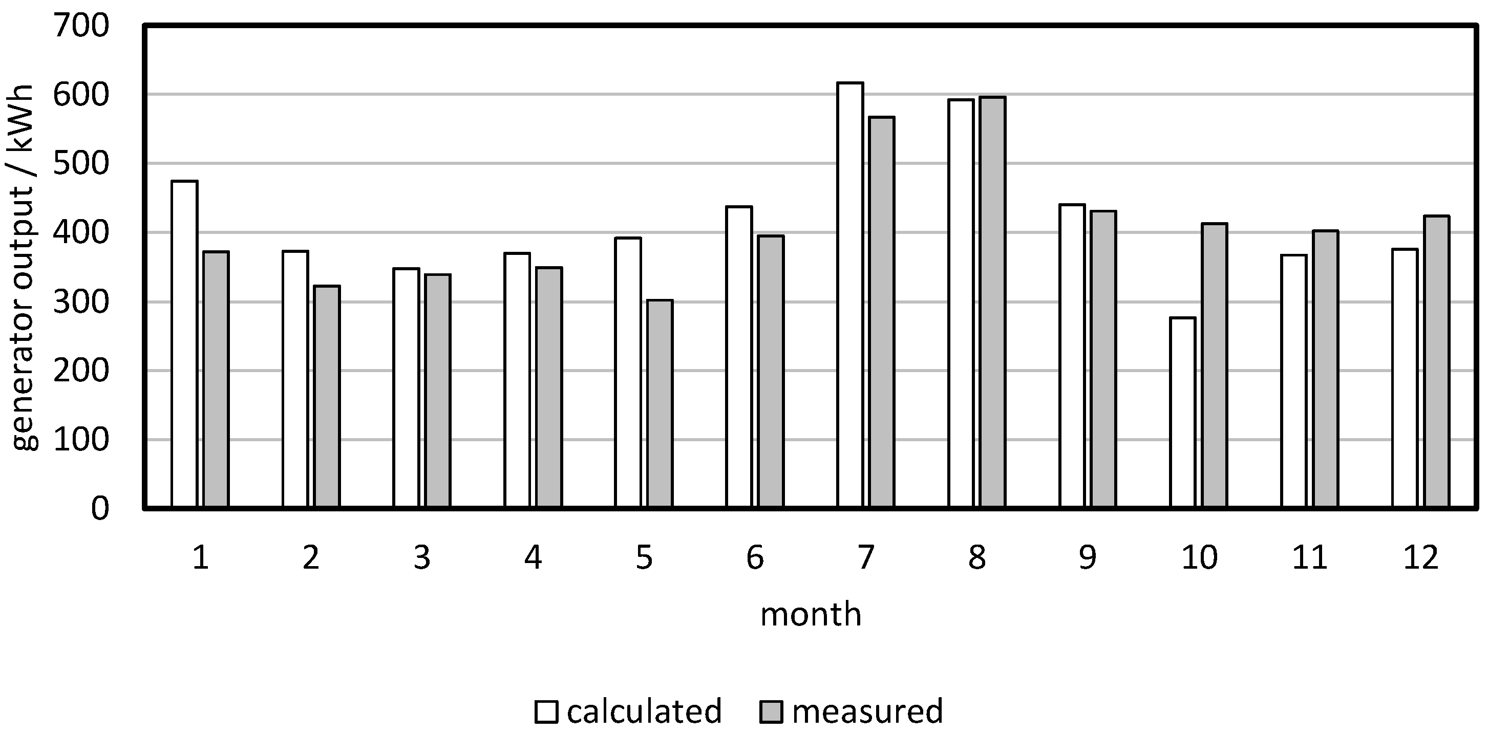
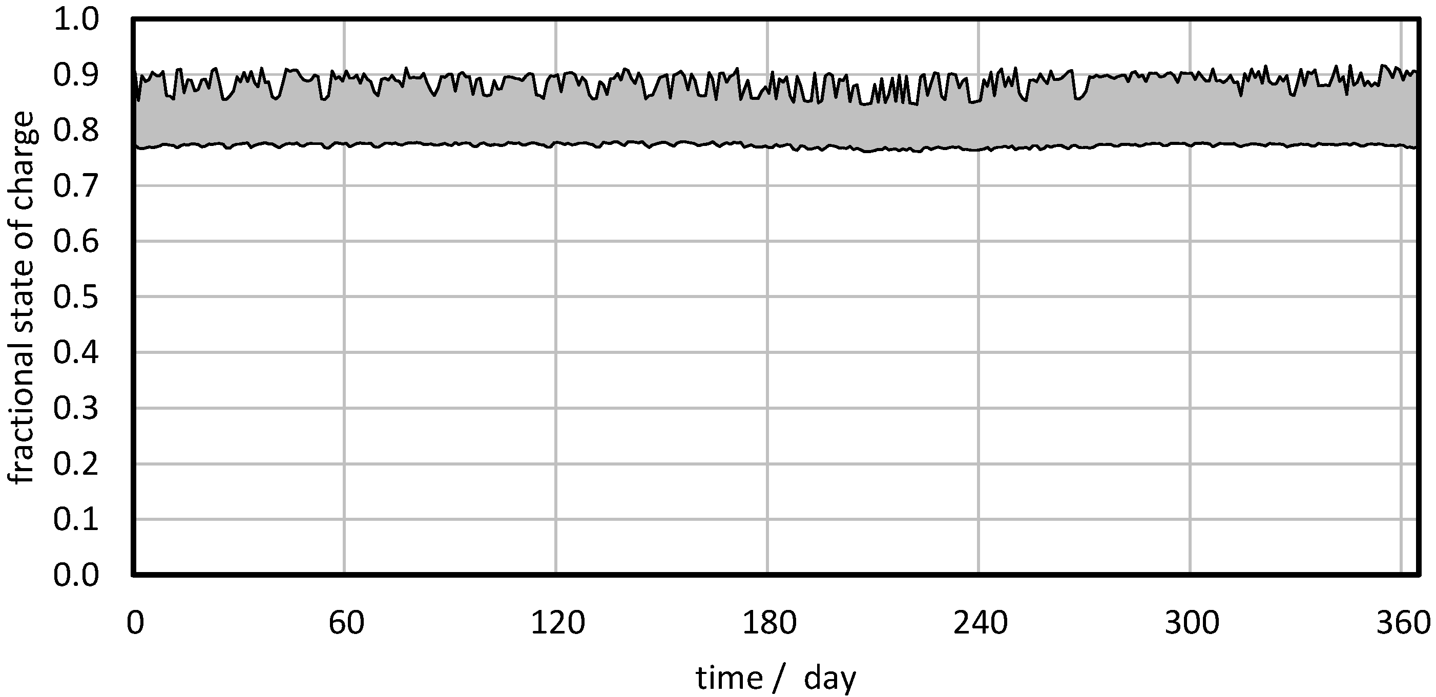
4.1. Custom Computational Model Validation with Experimental Data of the SOPE

Experimental data are only available for one of the observed configurations, marked with MEAS in Table 2. The system configuration is the same as in the SOPE, i.e., the system with an upgraded photovoltaic power supply. The integral parameters presented in Table 2 show that both the calculated (SOPE) total consumption and the generator output are in good agreement with the experimental values (MEAS). This confirms that the model is set up appropriately and can be used for the simulation of other configurations. A considerable amount of excess energy can be seen in the SOPE. This is the energy that cannot be either used or stored at the time when it is available. Figure 12 shows that the gen-set starts every morning to provide power, both for the hut and for charging the batteries. During the day, when solar power is available and its potential exceeds the consumption, the batteries are unable to store the excess energy, which is therefore not produced. This type of operation is also reported by the hut’s keepers, where the gen-set’s operation is regulated manually. Obviously, most of the energy stored in the batteries is produced by the gen-set instead of the photovoltaics. The high state of charge of the batteries provides an energy backup, but since the Lizara hut has two gen-sets, with one being redundant for normal operation, the batteries are not needed as an emergency backup. Therefore, the capacity could be utilized over a wider range.

It was found that this ineffectiveness in renewable energy production could be mitigated with a better charging strategy for the batteries using the gen-set. The results of the SOPE (Figure 14) reveal that the batteries’ fractional state of charge remains very high at all times. The batteries are not used in their complete operating range, which provides an opportunity to improve the system’s performance.

4.2. Improved Battery Charging Strategy in the SOPE+

With the current settings of the gen-set operation and the battery charging, the batteries are always fully charged when the gen-set is in operation and is suppling power to the load. If, at the same time, excess solar energy is available, it cannot be stored in the batteries. Thus, if the gen-set is not allowed to charge the batteries over a certain limit, the excess solar energy could be stored for later use. Figure 15 shows that limiting the charging of the batteries with the gen-set could free up capacity that could be used to store the excess solar energy. In this way, the gen-set’s operating time, as well as the fossil fuel consumption, decrease significantly and there is almost no excess energy (see Table 2 for SOPE+). In addition, the renewables penetration increases by 18.5%. Attention should be paid to the state of charge at the end of the generator’s scheduled operation, because the stored electricity must be sufficient to cover the night-time requirements for consumption. Fortunately, the night-time load is relatively constant and predictable, as already shown in Figure 5.

The employed regulation strategy results in a relatively low state of charge for the battery during the summer season, which might cause issues with the degradation of the battery. The average level of charge could be increased by additional charging with the gen-set, although this is not necessary from an energy balance point of view. To keep the batteries in good condition, a further improvement of the system’s regulation is possible, where an appropriate state of charge is maintained with the gen-set for the batteries.

4.3. The Simulation Results for the SOPB

To show the benefits of increasing the capacity of the PV panels, a simulation was also run with the configuration before the modifications, the SOPB. There are no experimental data for the SOPB, and we must use the TRANSYS model to calculate the energy balance. The results show that the gen-set must provide most of the electricity. In fact, less than 9% of all the generated electricity is provided by renewable sources. In addition, the generator produces much more electricity than the micro-grid system consumes, mostly due to the battery charging and the discharging inefficiency (Table 2).

4.4. Increased Power of the PV and Batteries’ Capacity to Increase Renewable Penetration

To reach the highest RES penetration, the power of the PV system and the capacity of the batteries must be increased. Two energy system configurations were simulated to approach (SOPEx2 with 93.2% renewable penetration) or to reach 100% renewables penetration in the RES case.

In the SOPEx2, the capacity of the PV system and batteries was doubled according to the SOPE, which is feasible, although undoubtedly an expensive approach. The renewables penetration increases considerably in SOPEx2, but the gen-set is still occasionally needed to bridge certain periods when neither solar nor stored energy is available.

For the MH system, it was found that fully renewable operation is possible if the PV system is increased by 200% and the capacity of the batteries by 400% compared to the SOPE. With this, it would be possible to store enough energy for longer periods of overcast weather, when solar energy is not available. Due to the considerably oversized PV capacity, the amount of energy that cannot be utilized is comparable to the total electrical energy consumed by the MH (Table 2). In this case, it might be reasonable to use this electricity for heating (powering electrical heaters) and thus reduce the consumption of LPG and mixed wood. With this approach, we could make the MH a fully stand-alone, RES-based, even sustainable, and near-zero-emission MH. Environmental impacts would still be present, if not so much because of the operational phase of the MH; they are present because of the manufacturing phase of the PV system, batteries, control units, etc., which uses some critical or rare materials, energy and processes that impact the environment and represent a burden. In the next section, an environmental assessment of all the observed configurations will be described and the best option regarding environmental impacts will be addressed.

5. Environmental Assessment

To evaluate the environmental performance of all the simulated configurations, the lifecycle assessment (LCA) methodology was used. LCA includes four phases: goal and scope, lifecycle inventory analysis (LCI), lifecycle impact assessment (LCIA) and interpretation of the results. It is conducted according to the ISO standards 14,040, 14,044 [47,48], and the International Reference Life Cycle Data System (ILCD) guidelines [49]. The topology of the energy system and the energy generation for all the configurations of the MH defined in the phase of modelling served as inputs for the LCA models.

5.1. Goal, Scope and Functional Unit

The functional unit is the electricity and the heat consumption (load) for the reference year (1 June 2018 to 31 May 2019) of the MH Lizara. The scope of the LCA study is from gate to gate, observing only the operational phase of MH Lizara. The manufacturing phase of the installed technologies (PV system, biomass boiler, LPG boiler, gen-set) is included, as well as the energy carriers (diesel, mixed wood, LPG), but the basic infrastructure of the MH and all the installed devices and facilities not connected to the energy generation system are excluded from the LCA.

In contrast to the energy balance modelling of different energy configurations, where the focus was only on the single-phase electricity generation system, the environmental assessment was performed for the complete energy distribution of the MH: for the single- and three-phase electricity generation systems, as well as the heat generation system with LPG and mixed wood. In addition, the transport of the energy carriers was included for all the observed configurations. With this approach, we can evaluate the environmental performance improvements of the MH operation phase due to the single-phase electricity generation optimization (from SOPE to SOPE+) and the upgrade (from SOPB to SOPE and further to SOPEx2 and RES). We can also evaluate the decrease in the environmental impacts due to (i) the PV installation or (ii) the heating system upgrade (heat recuperation chimney) in the SOPB configuration.

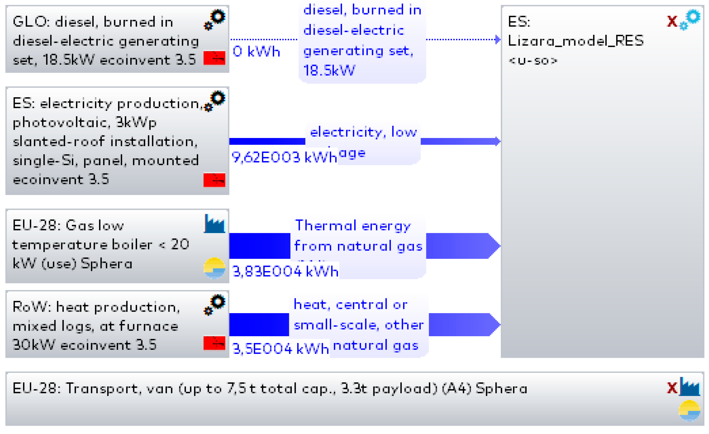
5.2. Life Cycle Inventory Analysis

5.2.1. Manufacturing and Operational Phase

The lifecycle inventory (LCI) analysis is based on the data from measurements, the basic defined topology of the energy system and the results of simulations for the observed configurations. The values of electricity generated with the gen-set or the PV system for all five configurations are presented in

Table 3. Lifecycle inventory data for all the modelled stand-alone energy configurations for 1 year of the hut’s operation.

	SOPB	SOPE	SOPE+	SOPEx2	RES	Process from Generic Database
Electricity (kWh)
PV slanted roof	791	4118	5793	8708	9615	ES: el. Prod., photovoltaic, 3 kWp slanted-roof installation, single-Si, panel, mounted, Ecoinvent 3.5
Diesel, 1-phase	8284	5064	3348	638	0	GLO: diesel, burned in diesel-electric generating set, 18.5 kW, Ecoinvent 3.5
Diesel, 3-phase	6439	6439	6439	6439	6439
Heat (kWh)
LPG boiler	73,292	35,040	35,040	35,040	35,040	EU-28: gas low-temperature boiler < 20 kW (use), Sphera
Mixed log chimney	350	38,252	38,252	38,252	38,252	RoW: heat production, mixed logs, 30 kW, Ecoinvent 3.5

, where the heat generated with the LPG boiler and the heat recuperated in the chimney using mixed logs are also listed. In the last column of Table 3, the processes used from the generic databases Ecoinvent 3.6 and GaBi Professional are listed [50,51]. These databases are the most suitable regarding the real power, type and installation specifics of the devices.

5.2.2. Transport Phase

The transport of fuels is the only one included in LCA models. Diesel and mixed logs (wood) are transported from Sabiñanigo, which is 73.3 km from MH Lizara, and the LPG is transported from Santurce, which is 296 km from MH Lizara. The LCI data for the transport phase in all five studied configurations are presented in

Table 4. Lifecycle inventory data for the transport of energy carriers to the hut for 1 year of the hut’s operation.

	Unit	SOPB	SOPE	SOPE+	SOPEx2	RES
Diesel, 1-phase	kg	2761.4	1687.7	1116.2	212.6	0.0
Diesel, 3-phase	kg	4907.7	3834.0	3262.5	2358.9	2146.3
Factor, diesel	km·kg	613,455	771,241	687,459	554,991	523,824
LPG	kg	6568	3140	3140	3140	3140
Factor, LPG	km·kg	1,944,128	929,440	929,440	929,440	929,440
Factor, total	km·kg	2,557,583	1,700,681	1,616,899	1,484,431	1,453,264

with the masses of the fuels to be transported and the product of distance and mass, which serves as the input for the LCA model. The process used for the transport phase is EU-28: Transport, van (up to 7.5 t total cap., 3.3 t payload) [50].

5.3. Lifecycle Impact Assessment Methodology

One of the major goals of the SustainHuts project is to assess and address the environmental impacts of MHs during their operating phase before (SOPB) and after (SOPE) the energy system’s adaptation [34]. Since the target emissions (CO₂, SO_X, NO_X and particles) defined in the project do not address all impact areas, the Centrum voor Milieukunde Leiden (CML) 2001 LCIA method was also used in this study to assess the environmental impacts in more detail (

Table 5. CML2001 environmental impact indicators [52].

	Abbr.	Name	Indicator	Units
Air/ Climate	GWP	Global Warming Potential	Greenhouse gas emissions	kg CO2-eq.
	AP	Acidification Potential	Air pollution	kg SO2-eq.
	POCP	Photochemical Ozone Creation Potential	Air pollution	kg Ethene-eq.
	ODP	Ozone-Layer Depletion Potential	Air pollution	kg R11-eq.
	HTP	Human Toxicity Potential	Toxicity	kg 1,4-DCB-eq.
Water	FAETP	Freshwater Aquatic Ecotoxicity Potential	Water pollution	kg 1,4-DCB-eq.
	MAETP	Marine Aquatic Ecotoxicity Potential	Water pollution	kg 1,4-DCB-eq.
	EP	Eutrophication Potential	Water pollution	kg PO4-eq.
Soil	TETP	Terrestrial Ecotoxicity Potential	Soil degradation and contamination	kg 1,4-DCB-eq.
Resources	ADP elem.	Abiotic depletion potential, elements	Resource depletion	kg Sb-eq.
	ADP fossil	Abiotic depletion potential, fossil	Resource depletion	MJ

).

5.4. Interpretation of the Results

To perform a critical interpretation of the environmental impacts, all the configurations were assessed using the same LCA base model (Figure 16) with the different boundary conditions presented in Table 3 and Table 4. The environmental impacts of five configurations were assessed and compared for 1 year of the hut’s operation. Observing only the target emissions and not the environmental impact indicators, we can see a gradual decrease in emissions from the SOPB at the beginning to an RES at the end. In contrast to CO₂, SO_X and NO_X in the case of particles (ppm2.5), there is a slight increase by 14% from the SOPB to the SOPE. After this, the emission of particles decreases towards the RES (by 18% from SOPE to RES).

In

Table 6. Comparison of environmental impact indicator values for all the observed configurations in the Lizara hut.

	Air/Climate					Water			Soil	Resources
	GWP 100 Years (kg CO2 eq.)	AP (kg SO2 eq.)	POCP (kg Ethene eq.)	ODP, Steady State (kg R11 eq.)	HTP inf. (kg DCB eq.)	FAETP inf. (kg DCB eq.)	MAETP inf. (kg DCB eq.)	EP (kg Phosphate eq.)	TETP inf. (kg DCB eq.)	ADP Elements (kg Sb eq.)	ADP Fossil (MJ)
SOPB	3.45 × 104	149	13.9	0.00246	2.90 × 103	1.68 × 103	3.32 × 106	37.4	52.6	0.0222	5.49 × 105
SOPE	2.26 × 104	130	21.4	0.00207	4.65 × 103	2.48 × 103	4.51 × 106	35.6	116.0	0.0296	3.42 × 105
SOPE+	2.11 × 104	115	20.0	0.00180	4.60 × 103	2.58 × 103	4.54 × 106	32.0	114.0	0.0314	3.21 × 105
SOPEx2	1.88 × 104	90.6	17.7	0.00136	4.56 × 103	2.78 × 103	4.64 × 106	26.3	111.0	0.0349	2.88 × 105
RES	1.83 × 104	85	17.1	0.00126	4.59 × 103	2.86 × 103	4.72 × 106	25.1	110.0	0.0363	2.80 × 105

a comparison of the environmental impact indicators for all the configurations is presented. In addition to the values, a color chart (green–orange–red) is used in each impact category to provide an additional visual effect for high (red) and low (green) relative values.

In the group of indicators affecting the air/climate, we can observe a positive trend from the SOPB to the RES that has a 100% renewable penetration. The global warming potential (GWP), acidification (AP) and ozone depletion (ODP) are reduced to 53%, 57% and 51%, respectively, in comparison to the SOPB, which is mostly fossil-fuel-based. In the case of POCP and HTP, the largest increase in values is from the SOPB to the SOPE; in the SOPE+, SOPEx2 and RES, the values are reduced. The reason for this is the additional installation of the PV system from 0.5 to 3.7 kWp and the installed heat recuperation chimney, which reduced the consumption of LPG by 52% from the SOPB to the SOPE, but increased the mixed wood consumption by 614%, according to the SOPB. The heat recuperation chimney is connected to the heat distribution system and can replace the LPG. The extra installed PV system has additional environmental impacts because of the PV manufacturing phase (in HTP, FATEP, MAETP and TETP indicator) and not due to its operation. In addition, the wood in the Lizara hut is combusted in an open fireplace that has characteristically very incomplete combustion, with lots of non-desirable emissions to the environment. This is why the reduction in LPG use from the SOPB to the SOPE by 52% and the reduction in the total diesel consumption by 22% do not decrease the POCP and HTP indicators, which are very much dependent on combustion.

The next group of indicators, which are connected to water pollution—Freshwater Aquatic Ecotoxicity (FAETP) and Marine Aquatic Ecotoxicity (MAETP)—show the same pattern of a large increase due to the uncontrolled wood combustion and the additional PV system being installed. At the same time, the Eutrophication (EP) is reduced to 67% in the RES in comparison to the SOPB. In the case of the EP indicator, the decrease in LPG and diesel consumption has a larger effect than the large increase in mixed wood use (combustion). In the Terrestrial Ecotoxicity (TETP), after a large increase from the SOPB to the SOPE due to a huge increase in wood use and the additional PV system installed, there is a slight decrease to the RES. In the case of the use of resources that is quantified with abiotic depletion (ADP elements and ADP fossil), there is a logical decrease in the ADP fossil that is linked with the reduced fossil fuel use (diesel, LPG and diesel for transport) from the SOPB to the RES. In the ADP elements, there is a visible increase in the indicator from the SOPB to the RES that is attributed to the additional PV system installed, i.e., 11.1 kWp in RES, and an increase in wood use. To perform a proper interpretation of the environmental impacts, the use of mass emissions is insufficient. The decrease in CO₂ emissions (

Table 7. Target emissions of the SustainHuts project in all the observed configurations in the Lizara hut.

	CO2, kg	CO2, %	SOX, kg	SOX, %	NOX, kg	NOX, %	ppm2.5, kg	ppm2.5, %
SOPB	3.30 × 104	100	27.3	100	232	100	27.4	100
SOPE	2.11 × 104	64	24.8	91	198	85	31.3	114
SOPE+	1.97 × 104	60	22.3	82	173	75	28.3	103
SOPEx2	1.74 × 104	53	18.6	68	134	58	23.6	86
RES	1.69 × 104	51	17.8	65	125	54	22.5	82

) has the same pattern as the GWP (

Table 8. The reduction/increase in the environmental impact indicators according to the SOPB.

	Air/Climate					Water			Soil	Resources
	GWP 100 Years	AP	POCP	ODP, Steady State	HTP inf.	FAETP inf.	MAETP inf.	EP	TETP inf.	ADP Elements	ADP Fossil
SOPB	100%	100%	100%	100%	100%	100%	100%	100%	100%	100%	100%
SOPE	66%	87%	154%	84%	160%	148%	136%	95%	221%	133%	62%
SOPE+	61%	77%	144%	73%	159%	154%	137%	86%	217%	141%	58%
SOPEx2	54%	61%	127%	55%	157%	165%	140%	70%	211%	157%	52%
RES	53%	57%	123%	51%	158%	170%	142%	67%	209%	164%	51%

). The same goes for the SO_X emissions that can be linked to the AP indicator. The NO_X and ppm2.5 emissions cannot otherwise be directly linked to the specific CML2001 indicator, but the particles (ppm2.5) increase from the SOPB to the SOPE indicates that the impact of the wood combustion process should be evaluated in more detail, as with the CML2001 LCIA methodology. Moreover, instead of an open-fire chimney, better-controlled combustion systems should be used to avoid a large increase in the FAETP, MAETP, HTP and TETP environmental indicators.

6. Discussion

To have 100% renewables penetration in the Lizara hut, the size of the PV system must be 11.1 kWh, with a battery capacity that is five times larger than in the SOPE and SOPE+. With such an over-sized system to meet the required load, higher costs are foreseen. A calculation of the investment costs (

Table 9. Investment costs in all the modelled configurations according to the SOPE investment costs and the size of the modelled configurations [38].

	SOPE	SOPE+	SOPEx2	RES
PV panels with regulator	5373.6 €	5373.6 €	12,311.1 €	18,466.6 €
Lead–acid batteries	9011.4 €	9011.4 €	18,022.7 €	45,056.8 €
Inverter unit	4975.2 €	4975.2 €	5475.2 €	6475.2 €
Improved charging strategy *	-	3000.0 €	3000.0 €	3000.0 €
Thermo-chimney with heat exchanger	5970.1 €	5970.1 €	5970.1 €	5970.1 €
Labor costs	968.0 €	968.0 €	1490.0 €	2215.0 €
TOTAL	26,298.3 €	29,298.3 €	46,269.1 €	81,183.7 €

* estimated cost.

) shows that the investment in the improved charging strategy in the SOPE+ is 10% larger than the investment for the “basic” SOPE. However, a 90% higher investment is required to double the size of the PV and batteries in the SOPEx2 and an investment as much as 270% higher is needed to achieve fully renewable operation in the RES. The input data for the calculation were taken from the actual investment in the SOPE and scaled according to the size of the installed equipment for other configurations.

To include the savings in costs for diesel, diesel for transport and LPG, we must introduce the price of diesel, LPG and wood. These are 0.85 €/liter for diesel, 1.62 €/kg for LPG and 0.02 €/kg for mixed wood for the Lizara hut owners, who have a special contract with the Federación Aragonesa de Montañismo (FAM) [53]. The calculated savings for 1 year would be 6541.1 €, 7112.6 €, 8016.2 € and 8228.8 € in the SOPE, SOPE+, SOPEx2 and RES, respectively. Using a simple payback methodology, this means 4 years of payback in the SOPE, 4.1 years in SOPE+, 5.8 years in SOPEx2 and 9.9 years in RES.

There is no single way to choose the optimal configuration if we combine technical, environmental and economic approaches. We should combine the technical feasibility, investment costs and payback time with the environmental impact indicators. The most effective solution in the Lizara hut that needs very little technical upgrade, has a significant reduction in environmental impacts (Table 8) and only prolongs the payback time from 4 years to 4.1 years is the SOPE+ case, which includes the improved charging strategy in addition to the SOPE. Looking for higher renewables penetration (Table 2) in the SOPEx2 (63.4%) or 100% in the case of the RES is much more expensive, with longer payback times and larger investments.

7. Conclusions

The workflow of combining energy system optimization and environmental and economic evaluations using a simple payback methodology was introduced in the case of the Lizara mountain hut. Five technically feasible configurations with increasing renewables penetration were modelled to obtain the required power and capacity of the basic components for electricity generation and storage. A lifecycle model was set up to evaluate the impacts of energy generation (electricity and heat) for 1 year of operation. In addition, the calculation of the investment costs for each configuration was made, fuel savings were evaluated, and a simple payback methodology used for the evaluation.

The results show that the recent upgrade of the energy system improved the renewables penetration from 8.7% to almost 44.9%. In addition, the optimization of the charging strategy, which was one of the main goals of the paper, improved the renewables penetration further to 63.4%, which was a large improvement that required a small investment. Higher renewables penetration results in lower environmental impacts. Global warming potential is decreased by 39% in the case of a system upgrade, including the improved charging strategy (SOPE+), compared to the state of play at the beginning (SOPB). The same pattern is noted for acidification, abiotic depletion, ozone depletion and eutrophication, which are consistently decreasing with system modifications, approaching 100% renewables penetration. The environmental indicators (FAETP, MAETP, HTP, TETP) that are influenced by the incomplete combustion process in the open fireplace, however, show a considerable increase for all the configurations, apart from the state of play at the beginning.

Reaching 100% renewables penetration is possible with a 3.1-times-higher investment compared the basic investment strategy realized in the SOPE, and the payback time is almost 10 years. Since the lifetime of the average MH is expected to be in the range of 50 years or more, all the calculated payback times are acceptable, but maintenance of the energy system should be included for longer operating periods. MHs are specific micro-grid energy systems, where environmental and technical assessments should always direct the investment. After all, we are dealing with very sensitive environments in the high mountains that should be preserved, and so cost should not be the most important issue.

References

1. Mori, M.; Gutiérrez, M.; Casero, P. Micro-grid design and life-cycle assessment of a mountain hut’s stand-alone energy system with hydrogen used for seasonal storage. Int. J. Hydrogen Energy 2021, 46, 29706–29723. [Google Scholar] [CrossRef]
2. Goymann, M.; Wittenwiler, M.; Hellweg, S. Environmental decision support for the construction of a “green” mountain hut. Environ. Sci. Technol. 2008, 42, 4060–4067. [Google Scholar] [CrossRef] [PubMed]
3. Schweizer-Ries, P. Decentralized Energy Use in Mountain Regions. Mt. Res. Dev. 2001, 21, 25–29. [Google Scholar] [CrossRef]
4. Tong, Z.; Zhang, K.M. The near-source impacts of diesel backup generators in urban environments. Atmos. Environ. 2015, 109, 262–271. [Google Scholar] [CrossRef]
5. Shah, S.D.; Cocker, D.R.; Johnson, K.C.; Lee, J.M.; Soriano, B.L.; Miller, J.W. Emissions of regulated pollutants from in-use diesel back-up generators. Atmos. Environ. 2006, 40, 4199–4209. [Google Scholar] [CrossRef]
6. Günkaya, Z.; Özdemir, A.; Özkan, A.; Banar, M. Environmental Performance of Electricity Generation Based on Resources: A Life Cycle Assessment Case Study in Turkey. Sustainability 2016, 8, 1097. [Google Scholar] [CrossRef] [Green Version]
7. Smith, C.; Burrows, J.; Scheier, E.; Young, A.; Smith, J.; Young, T.; Gheewala, S.H. Comparative Life Cycle Assessment of a Thai Island’s diesel/PV/wind hybrid microgrid. Renew. Energy 2015, 80, 85–100. [Google Scholar] [CrossRef]
8. Communication from the Commision: A Roadmap for Moving to a Competitive Low Carbon Economy in 2050; European Commission: Brussels, Belgium, 2011; Volume 34, pp. 1–34, COM (2011) 112 Final.
9. European Commission. The European Green Deal; European Commission: Brussels, Belgium, 2019; Volume 53. [Google Scholar]
10. Mori, M.; Sekavčnik, M.; Drobnič, B. Integration of numerical and experimental approach in life cycle assessment of stand-alone microgrid system. In Proceedings of the 16th SDEWES Conference on Sustainable Development of Energy, Water and Environment Systems; Ban, M., Ed.; Faculty of Mechanical Engineering and Naval Architecture: Dubrovnik, Croatia, 2021; pp. 1–14. [Google Scholar]
11. Chauhan, A.; Saini, R.P. Renewable energy based power generation for stand-alone applications: A review. In Proceedings of the 2013 International Conference on Energy Efficient Technologies for Sustainability, Nagercoil, India, 10–12 April 2013; pp. 424–428. [Google Scholar] [CrossRef]
12. Khatib, T.; Ibrahim, I.A.; Mohamed, A. A review on sizing methodologies of photovoltaic array and storage battery in a standalone photovoltaic system. Energy Convers. Manag. 2016, 120, 430–448. [Google Scholar] [CrossRef]
13. Zomer, C.; Custódio, I.; Goulart, S.; Mantelli, S.; Martins, G.; Campos, R.; Pinto, G.; Rüther, R. Energy balance and performance assessment of PV systems installed at a positive-energy building (PEB) solar energy research centre. Sol. Energy 2020, 212, 258–274. [Google Scholar] [CrossRef]
14. Delille, G.; François, B.; Malarange, G. Dynamic frequency control support by energy storage to reduce the impact of wind and solar generation on isolated power system’s inertia. IEEE Trans. Sustain. Energy 2012, 3, 931–939. [Google Scholar] [CrossRef]
15. Bernal-Agustín, J.L.; Dufo-López, R. Simulation and optimization of stand-alone hybrid renewable energy systems. Renew. Sustain. Energy Rev. 2009, 13, 2111–2118. [Google Scholar] [CrossRef]
16. Mathiesen, B.V.; Lund, H. Comparative analyses of seven technologies to facilitate the integration of fluctuating renewable energy sources. IET Renew. Power Gener. 2009, 3, 190–204. [Google Scholar] [CrossRef]
17. Lacko, R.; Drobnič, B.; Mori, M.; Sekavčnik, M.; Vidmar, M. Stand-alone renewable combined heat and power system with hydrogen technologies for household application. Energy 2014, 77, 164–170. [Google Scholar] [CrossRef]
18. Lacko, R.; Drobnič, B.; Sekavčnik, M.; Mori, M. Hydrogen energy system with renewables for isolated households: The optimal system design, numerical analysis and experimental evaluation. Energy Build. 2014, 80, 106–113. [Google Scholar] [CrossRef]
19. Bojić, M.; Nikolić, N.; Nikolić, D.; Skerlić, J.; Miletić, I. Toward a positive-net-energy residential building in Serbian conditions. Appl. Energy 2011, 88, 2407–2419. [Google Scholar] [CrossRef]
20. Mulleriyawage, U.G.K.; Shen, W.X. Optimally sizing of battery energy storage capacity by operational optimization of residential PV-Battery systems: An Australian household case study. Renew. Energy 2020, 160, 852–864. [Google Scholar] [CrossRef]
21. Ramirez Camargo, L.; Nitsch, F.; Gruber, K.; Dorner, W. Electricity self-sufficiency of single-family houses in Germany and the Czech Republic. Appl. Energy 2018, 228, 902–915. [Google Scholar] [CrossRef]
22. Cabezas, M.D.; Wolfram, E.A.; Franco, J.I.; Fasoli, H.J. Hydrogen vector for using PV energy obtained at Esperanza Base, Antarctica. Int. J. Hydrog. Energy 2017, 42, 23455–23463. [Google Scholar] [CrossRef]
23. Ulleberg, Ø.; Nakken, T.; Eté, A. The wind/hydrogen demonstration system at Utsira in Norway: Evaluation of system performance using operational data and updated hydrogen energy system modeling tools. Int. J. Hydrog. Energy 2010, 35, 1841–1852. [Google Scholar] [CrossRef]
24. Bourdeau, M.; Basset, P.; Beauchêne, S.; Da Silva, D.; Guiot, T.; Werner, D.; Nefzaoui, E. Classification of daily electric load profiles of non-residential buildings. Energy Build. 2021, 233, 110670. [Google Scholar] [CrossRef]
25. Benlahbib, B.; Bouarroudj, N.; Mekhilef, S.; Abdeldjalil, D.; Abdelkrim, T.; Bouchafaa, F.; Lakhdari, A. Experimental investigation of power management and control of a PV/wind/fuel cell/battery hybrid energy system microgrid. Int. J. Hydrog. Energy 2020, 45, 29110–29122. [Google Scholar] [CrossRef]
26. Zhang, Y.; Wei, W. Model construction and energy management system of lithium battery, PV generator, hydrogen production unit and fuel cell in islanded AC microgrid. Int. J. Hydrog. Energy 2020, 45, 16381–16397. [Google Scholar] [CrossRef]
27. Paul Ayeng’o, S.; Axelsen, H.; Haberschusz, D.; Sauer, D.U. A model for direct-coupled PV systems with batteries depending on solar radiation, temperature and number of serial connected PV cells. Sol. Energy 2019, 183, 120–131. [Google Scholar] [CrossRef]
28. Cho, D.; Valenzuela, J. Optimization of residential off-grid PV-battery systems. Sol. Energy 2020, 208, 766–777. [Google Scholar] [CrossRef]
29. Soudan, B.; Darya, A. Autonomous smart switching control for off-grid hybrid PV/battery/diesel power system. Energy 2020, 211, 118567. [Google Scholar] [CrossRef]
30. Haratian, M.; Tabibi, P.; Sadeghi, M.; Vaseghi, B.; Poustdouz, A. A renewable energy solution for stand-alone power generation: A case study of KhshU Site-Iran. Renew. Energy 2018, 125, 926–935. [Google Scholar] [CrossRef]
31. EU Project: Sustainhuts-Demonstrative Project Which Aims to Reduce CO2 Emissions in Natural Environments Acting in Huts; G.A. LIFE15 CCA/ES/000058; European Commission: Brussels, Belgium, 2016.
32. Mori, M. Life Cycle Model (LCA) of RE Technologies Implementation and Sensitivity Analysis: Life Sustainhuts: Sustainable Mountain Huts in Europe: Life Cycle Assessment and Environmental Analysis; Faculty of Mechanical Engineering: Ljubljana, Slovenia, 2020. [Google Scholar]
33. Mori, M. LCA Model of Case Study with All Listed Technologies Implemented: Life Sustainhuts: Sustainable Mountain Huts in Europe: Life Cycle Assessment and Environmental Analysis; Faculty of Mechanical Engineering: Ljubljana, Slovenia, 2020. [Google Scholar]
34. Casero, P. Sustainable Mountainhuts in Europe, LIFE15 CCA/ES/000058; European Commission: Brussels, Belgium, 2016. [Google Scholar]
35. Global Solar Atlas. Available online: https://globalsolaratlas.info/map (accessed on 17 July 2021).
36. Bourdeau, M.; Nefzaoui, E.; Guo, X.; Chatellier, P. Modeling and forecasting building energy consumption: A review of data- driven techniques. Sustain. Cities Soc. 2019, 48, 101533. [Google Scholar] [CrossRef]
37. Panapakidis, I.P.; Papadopoulos, T.A.; Christoforidis, G.C.; Papagiannis, G.K. Pattern recognition algorithms for electricity load curve analysis of buildings. Energy Build. 2014, 73, 137–145. [Google Scholar] [CrossRef]
38. Gutiérrez, M.; Casero, P. Life15 CCA/ES/000058 Life Sustainhuts: Sustainable Mountain Huts in Europe D1.4 Third Monitoring Report_Spanish Huts; European Commission: Brussels, Belgium, 2020. [Google Scholar]
39. Knight, K.M.; Klein, S.A.; Duffie, J.A. A methodology for the synthesis of hourly weather data. Sol. Energy 1991, 46, 109–120. [Google Scholar] [CrossRef]
40. Graham, V.A.; Hollands, K.G.T.; Unny, T.E. Stochastic variation of hourly solar radiation over the day. Adv. Sol. Energy Technol. 1988, 3796–3800. [Google Scholar] [CrossRef]
41. Degelman, L.O. A Weather Simulation Model for Building Energy Analysis. In Proceedings of the ASHRAE Transaction, Symposium on Weather Data; Pennsylvania State University: State College, PA, USA, 1976; pp. 435–447. [Google Scholar]
42. Gansler, R.A.; Klein, S.A.; Beckman, W.A. Assessment of the accuracy of generated meteorological data for use in solar energy simulation studies. Sol. Energy 1994, 53, 279–287. [Google Scholar] [CrossRef]
43. TESS Component Library Package—TESS Libraries|TRNSYS: Transient System Simulation Tool; TESS-Thermal Energy Systems Specialists: Madison, WI, USA, 2012.
44. Renewables.ninja. Available online: https://www.renewables.ninja/ (accessed on 10 December 2021).
45. Molod, A.; Takacs, L.; Suarez, M.; Bacmeister, J. Development of the GEOS-5 atmospheric general circulation model: Evolution from MERRA to MERRA2. Geosci. Model Dev. 2015, 8, 1339–1356. [Google Scholar] [CrossRef] [Green Version]
46. Welcome|TRNSYS: Transient System Simulation Tool. Available online: http://www.trnsys.com/ (accessed on 17 July 2021).
47. International Organisation for Standardisation. ISO 14040 (2006a): Environmental Management—Life Cycle Assessment—Principles and Framework; International Organisation for Standardisation: Geneva, Switzerland, 2006. [Google Scholar]
48. International Organisation for Standardisation. ISO 14044: Environmental Management—Life Cycle Assessment—Requirements and Guidelines; International Organisation for Standardisation: Geneva, Switzerland, 2006. [Google Scholar]
49. European Commission; Joint Research Centre; Institute for Environment and Sustainability. General Guide for Life Cycle Assessment—Detailed Guidance; Publications Office of the European Union: Luxembourg, 2010; ISBN 978-92-79-19092-6. [Google Scholar]
50. GaBi Databases: Professional Database; Sphera Solutions: Leinfelden-Echterdingen, Germany, 2018.
51. Ecoinvent 3.6: The Latest Version of the Ecoinvent Database Features More Than 2200 New and 2500 Updated Datasets; Ecoinvent: Zurich, Switzerland, 2019.
52. Mori, M.; Lotrič, A.; Stropnik, R.; Drobnič, B.; Sekavčnik, M. LIFE15 CCA/ES/000058 LIFE SUSTAINHUTS: Life Cycle Assessment and Environmental Analysis, C5.2 Life Cycle Inventory Analysis (LCIA): Mass and Energy Balances of Mountain Huts; Faculty of Mechanical Engineering: Ljubljana, Slovenia, 2017. [Google Scholar]
53. Federación Aragonesa de Montañismo. Available online: https://www.fam.es/ (accessed on 6 September 2021).
Figure 1. Electricity scheme of the Lizara hut (DL is the data logger).
Energies 15 00202 g001
Figure 2. Monthly energy consumption and production with diesel generator.
Energies 15 00202 g002
Figure 3. Seasonal variation in the measured load.
Energies 15 00202 g003
Figure 4. Daily variation in the measured load.
Energies 15 00202 g004
Figure 5. Average normalized daily load profile and the proposed simplified profile.
Energies 15 00202 g005
Figure 6. Seasonal variation in the normalized maximum daily loads.
Energies 15 00202 g006
Figure 7. Comparison of the actual and proposed simplified normalized maximum loads.
Energies 15 00202 g007
Figure 8. Comparison of the measured and simulated loads.
Energies 15 00202 g008
Figure 9. Duration curve of the measured and simulated loads.
Energies 15 00202 g009
Figure 10. Reference meteorological data used in the developed models.
Energies 15 00202 g010
Figure 11. System configuration in TRNSYS software environment for the simulations.
Energies 15 00202 g011
Figure 12. Power production and charge on the batteries for the SOPE for 1 week.
Energies 15 00202 g012
Figure 13. Measured and calculated monthly generator output for the SOPE.
Energies 15 00202 g013
Figure 14. Daily low and high limits of the fractional state of charge of the batteries in the SOPE.
Energies 15 00202 g014
Figure 15. Daily low and high limits of the fractional state of the charge of the batteries in the SOPE+.
Energies 15 00202 g015
Figure 16. General LCA model adapted for the RES case of the Lizara hut.
Energies 15 00202 g016