Article

Statistical Investigation of Climate Change Effects on the Utilization of the Sediment Heat Energy

1
Department of Electrical Engineering and Energy Technology, School of Technology and Innovations, University of Vaasa, 65101 Vaasa, Finland
2
Department of Civil Engineering, Aalto University, 00076 Espoo, Finland
3
Faculty of Science and Technology, Middlesex University, London NW4 4BT, UK
*
Author to whom correspondence should be addressed.
Energies 2022, 15(2), 435; https://doi.org/10.3390/en15020435
Submission received: 10 December 2021 / Revised: 3 January 2022 / Accepted: 4 January 2022 / Published: 7 January 2022

Abstract

:
Suvilahti, a suburb of the city of Vaasa in western Finland, was the first area to use seabed sediment heat as the main source of heating for a high number of houses. Moreover, in the same area, a unique land uplift effect is ongoing. The aim of this paper is to solve the challenges and find opportunities caused by global warming by utilizing seabed sediment energy as a renewable heat source. Measurement data of water and air temperature were analyzed, and correlations were established for the sediment temperature data using Statistical Analysis System (SAS) Enterprise Guide 7.1. software. The analysis and provisional forecast based on the autoregression integrated moving average (ARIMA) model revealed that air and water temperatures show incremental increases through time, and that sediment temperature has positive correlations with water temperature with a 2-month lag. Therefore, sediment heat energy is also expected to increase in the future. Factor analysis validations show that the data have a normal cluster and no particular outliers. This study concludes that sediment heat energy can be considered in prominent renewable production, transforming climate change into a useful solution, at least in summertime.

1. Introduction

Sediment energy is renewable energy because the thermal energy of the sediment layer mainly originates from the Sun (with seasonal storage and loss). A minor portion is from the Earth’s own geothermal energy. The flux in solar energy is from four to five orders of magnitude larger than the flux in geothermal heat on a normal land surface [1,2,3]. The combination of geothermal energy and solar energy as an energy source is called geoenergy [4]. Sediment heat is usually collected by the pipes that are horizontally installed into the sediment layer, and circulating heat-extracting liquid in the pipes. The temperature profile of the sediment is collected using the Distributed Temperature Sensing (DTS) method [5,6]. A more detailed review and description of the DTS is presented in an IEEE journal publication by Ukil et al. [6]. The seawater battery for deep water applications has been studied by Wilcock and Kauffman [7]. The sediment nutrient contents of total carbon and nitrogen variation due to human activities has been investigated by Wang et al. [8]. On the other hand, Reimers et al. [9] investigated a different way of harvesting energy from Marchine sediment–water interface.
Hiltunen et al. [10] show a potential for sediment renewable carbon-free energy for heat production in the local area. The use of thermal energy from the solid organic sediment layer at the bottom of water bodies via heat-collection pipes, heat-carrier liquids, and heat pumps is one of the new carbon-free ways to produce energy that was investigated by the University of Vaasa. Sediment energy can be used for cooling in summer and heating in winter, as shown in the Suvilahti shallow bay in the city of Vaasa, Finland [1,10,11]. Mäkiranta et al. [12] studied the correlation between the temperatures of air, heat carrier liquid, and seabed sediment in a renewable low-energy network. In their investigation, they confirmed correlations between the air temperature, heat carrier liquid temperature after 2 months, and the sediment temperature. A further study on seabed energy as an annual renewable heat source demonstrated that the collection of heat energy does not cause any permanent cooling of the sediment, and that the energy is sustainable. However, the air temperature influences the water and sediment temperature [13]. Global warming causes an air temperature increase and, in turn, an increase in the water temperature [11]. Further economic feasibility studies show that the collection depth has to be at least 3 m below the sea bottom [13]. Sediment thermal conductivity values have been noted to increase and stabilize in deeper layers. The depth of stable thermal conductivity values was related to the sedimentary environment [14]. Thermal conductivity and thermal diffusivity increase with increasing depth below the seafloor because they are negatively correlated with porosity [15]. On the other hand, these relations are also important in other areas of study, such as climate change and water quality analysis.
Depending on the lake type, the mixing and penetration of the solar energy to the bottom of the lake differs. In the meromictic lake experiment in [2], the low or non-mixing conditions of the lake water caused less annual temperature fluctuation than that observed in deep water. The particular lake water they studied (Stewart’s Dark Lake) had a high concentration of humic colloids or colored materials, thus resulting in a low level of solar radiation penetration. This shows that the sediment water energy that builds up from geothermal and solar energy depends on the type of water body [2]. Mixing, circulation patterns in the lake, and direct isolation of solar energy can heat and/or cool the bottom water of a lake. Moreover, direct heating from solar energy is influenced by the depth of the lake water. The water body and bottom sediment of shallow lakes can easily be heated. The results of Guo and Ma [16] also show that the temperature of seawater is evidently influenced by the sediment–water heat exchange, and that tidal sediment was a heat source providing warmth to the seawater. Golosov and Kirillin [17] studied two lakes in Russia and Germany for their sediment conductivity, based on a model that uses lake water temperature without any data on sediment thermal properties. This seems very useful for the sediment-heat energy analysis. Lake sediments play an interesting and appreciable role in heat transfer and exchange between lakes and the lower atmosphere (ground earth) in the majority of lakes [17]. Pivato et al. [18] has also concluded that heat flux at the sediment–water interface is crucial for soil temperature dynamics. Golosov and Kirillin [17] state that their model can be used effectively to estimate the effect of climate change on lakes, and can also be used to analyze the backward effect of lakes on the climate system. Considering the benefits of near-bottom temperature analysis (at the lake sediment boundary), crustal temperatures can be used to monitor the activity of the benthic community and biochemical processes. This is especially important in ice-covered lakes, where this comprises a major heat source in seasonal periods [17]. According to Hamilton et al. [19], time-varying sediment heat flux can especially affect the water temperature in ice-covered water bodies. Heat flows from the sediments to the water column and from the water to the ice, which occurs during ice-cover periods [20].
The sediment heat budget becomes more significant as the average depth of a lake decreases and is more significant nearer the shores than in deep water [2]. Smith [21] found that measurements of water–sediment heat exchange can show differences in temperature values due to the different time of year in which they are recorded, which makes it difficult to compare them. The results of Tsay et al. [22] suggest that the accurate simulation of thermal stratification in shallow transparent lakes requires consideration of sediment heat flux. In addition, some studies show that activities and construction in a water body can affect the water quality for some period of time. The buildup of sediment heat can also affect the water quality, and this can be considered as one kind of environmental risk caused by renewable energy use and production. In previous conference papers concerning Ostrobothnia, it has been indicated that constrictions that take place in the water area influence the water-quality parameters. Sediment energy is one of the important types of seaside energy solutions; therefore, it is important to consider it in the context of further developments.
The objective of this study is to obtain new data on a unique heating and cooling system in order to describe its status and operation, temperature distributions, correlation tests, and dependency analysis. Temperature versus distance measurements can provide data to optimize the size of the installation. The novelty of this study is in its researching a possible connection between climate change and the utilization of seabed sediment heat collection. This would help in the planning of new constructions in the future.
The research questions raised in this study are:
(1)
Is there a correlation between different months vs. the distance from shore in sediment temperature? At what distance is the maximum sediment heat energy production possible?
(2)
Can climate change be advantageous for using sediment heat energy?
(3)
What are the benefits for using sediment heat energy if weather temperatures become warmer in summer and winter?
A research gap is expected to be filled by examining the correlation between distance from shore and sediment temperature variations. The climate change effect can be advantageous for renewable energy production. Furthermore, renewable energy production, which uses climate change advantages, can potentially be used in the fight against climate change.

2. Materials and Methods

2.1. Data Collection Sites, Method, Descriptions and Validations

A housing fair was arranged in Suvilahti, Vaasa, in 2008. New houses were designed to utilize the annually reloaded heat energy from seabed sediment as heating and cooling energy. The energy was mainly generated by the Sun and collected through heat collection pipes filled with heat collection fluid. A unique low-energy network was built to cover the heating and cooling demand of 42 detached houses.
The total length of the Suvilahti seabed sediment heat collection pipeline was about 8 km (12 × 300 m and 14 × 300 m), and it was installed in the solid clay layer, horizontally into the seabed sediment, by a horizontal drilling machine (Figure 1). The position of the pipes was at 3–4 m depth from the sea bottom of the Gulf of Bothnia. Sediment heat is extracted via this heat-collector pipe field in the sediment layer and heat pumps inside the individual houses. The network is also used to cool houses in the summertime.
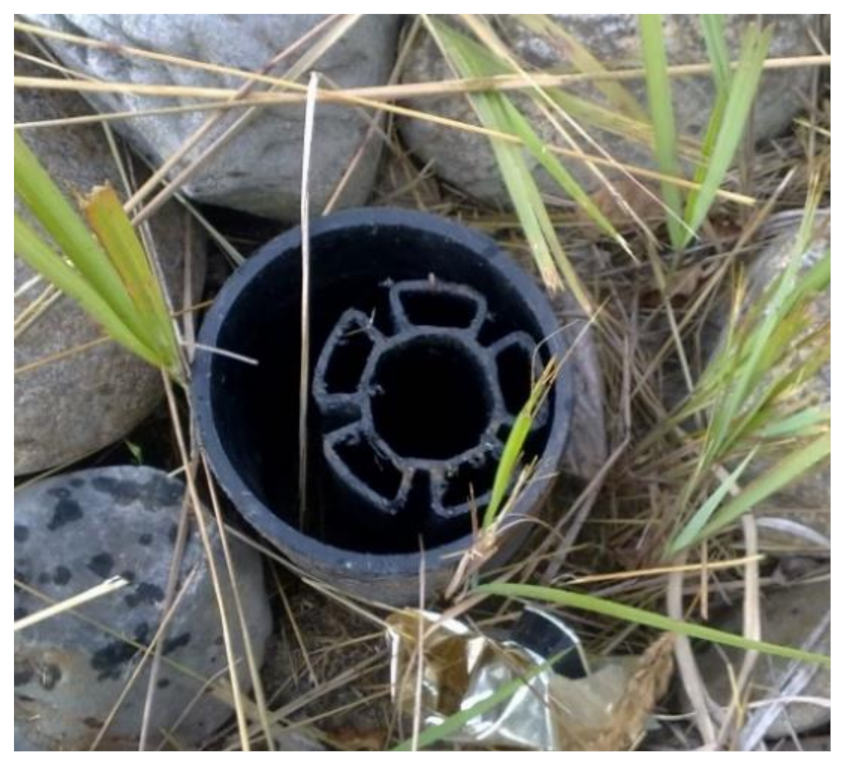
Heat carrier fluid runs in the brackets of the pipe on the outer casing gathering thermal energy. When the collection fluid reaches the end of the pipe, it returns to the shore through the middle of the pipe to release thermal energy for the heat pump. After that, the fluid begins the cycle again (Figure 2).
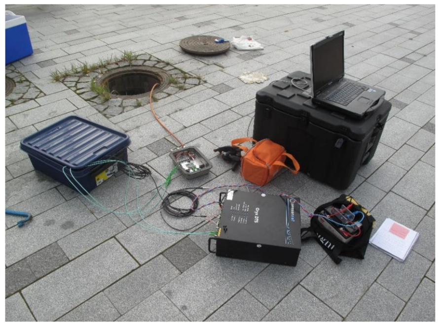
Sediment temperatures were measured using a distributed temperature-sensing (DTS) method in Suvilahti. A fiberglass cable was used as a linear temperature sensor. The cable was installed on the surface of one heat-collection pipe during the building process of the Housing Fair area. The total length of the cable temperature sensor was 300 m. The measurement device and calibration configurations are shown in Figure 3. Measurements were carried out once per month because of the delay in the air temperature influence on sediment temperature. Sediment heat temperature data used in this analysis were recorded during the years 2013–2016 and for only one month in 2018.
Mäkiranta [5] has described the distributed temperature sensing (DTS) method and its limitations in her thesis. DTS measurements were calibrated during each measurement with the help of Pt100 (accuracy ± 0.25 °C) point sensors. A separate patch cable was used to make the connection for calibrations. The patch cable was routed into an ice-bath to ensure the temperature data validity in these double-ended measurements. The sensor cables in the seabed sediment were installed on the outside of the system’s heat-collection pipes, which contain the heat carrier fluid. The validity of the sediment temperature data can still be regarded as reasonable due to the fact that the fluid’s influence on the surrounding sediment temperature can be expected to be quite small. The forecasted data have limitations in ARIMA modeling. Only 60 years of data were used to predict 40 years forward. This does not satisfy the modeling prediction requirements. However, a similar result to our forecasts was found in IPCC (2021) publications, which is why they are presented. Weather data were collected from the Vaasa airport weather station for the years 1959–2019. The weather data were collected by Finnish Metrological Institute. The water temperature data were taken from water quality data collected by the ELY-keskus (Center for Economic Development, Transport and the Environment) at the Eteläinen Kaupunkiselkä 1 sampling point in the city of Vaasa between 1962 and 2018. The water data were used in autoregression integrated moving average (ARIMA) forecast modeling. However, it is noted that the water sampling point was different from the sediment energy installation point because there is no long-term water quality measurement data that correspond with the sediment energy installation points. The forecasted data have limitations in ARIMA modeling. Only 60 years of data were used to predict 40 years forward, which, again, does not satisfy the modeling prediction requirements. However, it was a similar result to that found in IPCC (2021) publications.

2.2. General Statistical Analysis Method

The analysis was conducted using SAS Enterprise Guide 7.1 software. The statistical analysis conducted in SAS includes descriptive analysis, dependency analysis, autoregression integrated moving average (ARIMA) forecast modelling, and factor analysis. All analyses were conducted using the prescribed software procedures for each tool, and additional detailed information can be found at [23]. However, the general procedure used in the statistical analyses was based on the eight steps of general data analysis procedure (Dytham [24]) described below:
(1)
Decide specific points of interest;
(2)
Formulate several hypotheses;
(3)
Design and choose the necessary data and parameters for analyses;
(4)
Collect dummy data to form approximate values based on what was expected to be obtained—some of our original data were used as dummy data during this analysis;
(5)
Select appropriate tests;
(6)
Carry out the test(s) using the dummy data;
(7)
If there are problems, go back to step 3 (or 2); otherwise, proceed to use real data;
(8)
Carry out the test(s) using the real data and report the findings and/or return to step 2.

3. Results

3.1. Summary of Statistics

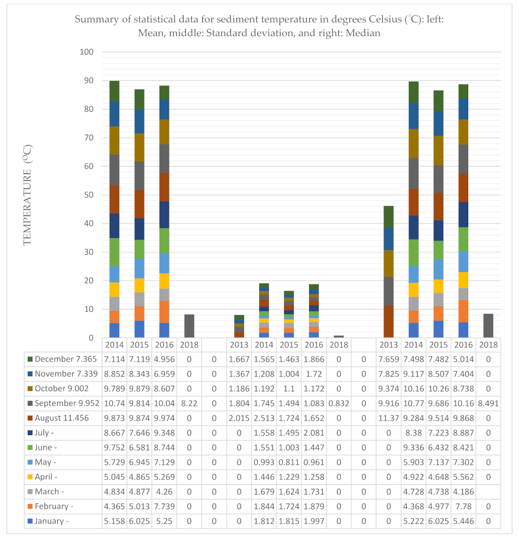
The sediment temperature measurement distances from the shore stretched 0–300 m towards the center of the water body. The normality of the data was checked at the beginning. All of the temperature data were found to be non-normal for all years and months, except for the distributions of distance measurements and in the Suvilahti Liito-oravankatu location for August 2013 and August 2015. Figure 4 shows the 2016 September data measured on 3 October 2016, and the December 2016 data measured on 10 January 2017. The bold highlighted data for Vaasa, Suvilahti, Ketunkatu in Figure 4 shows incremental or decremental increases in the years from 2013 to 2018. No yearly pattern was noticed at Vaasa, Suvilahti, Liito-oravankatu. In Figure 4, the mean sediment temperature data for February and May show an incremental increase in line with the year of sampling. The January data standard variation shows an increment in variation with increasing years. However, September shows a decline in the standard variation level with increasing years.
Median values show incremental increases in the months of February and May, and a decrement was noticed in December. The average highest sediment temperature was recorded from June to December in almost all of the recorded years. Medians also show similar results to the average values. January and August standard variation values were among the highest in all of the years recorded in Ketunkatu. Figure 1 shows the summary of statistical data for sediment temperature at the Suvilahti, Ketunkatu site. Here, only the main results are presented. The highest mean and median sediment temperatures were observed in August 2013 at Ketunkatu. July 2016 showed the highest standard variations for this site. The lowest mean and median for sediment temperatures observed at Ketunkatu were seen in February 2014, and the lowest standard deviation was observed in May 2015.
A summary is given of the statistical data for sediment temperature at the Suvilahti, Liito-oravankatu site. Standard variation values from October to December were the highest in all years in Liito-oravankatu. No clear increment or decrement pattern can be seen in the data. The highest average/mean and median sediment temperature values were observed from July to September throughout the years. The highest mean and median sediment temperatures at Liito-oravankatu were observed in September 2014. October 2016 showed the highest standard variations at this site. The lowest mean was seen in January 2014 and the lowest median was in March 2014. The lowest standard deviation was observed in August 2013.

3.2. Dependency Analysis

The correlation uses hypotheses that either confirm or falsify. The null hypothesis is H0: the population correlation is zero (i.e., there is no linear relationship). The alternative hypothesis is H1: the population correlation is not zero. If the correlation result is not statistically significant it means the null hypothesis (H0) is accepted and the alternative hypothesis (H1) is rejected. If it is statistically significant, then the alternative hypothesis is accepted and the null hypothesis is rejected. Pearson’s correlation is an appropriate analysis for this kind of non-ranked data, but to use Spearman’s rank correlation, the data must be ranked beforehand.
With the exception of a few months, the results show statistically significant Pearson’s correlations in months vs. distances from the shore towards to center of the water body. June, July, August, and September vs. distance correlations were found to be negative (Table 1). During these months, as the distance from the shore increases the temperature declines significantly. A similar finding was also found in October 2016, but the sampling day is closer to September than the middle of October, and is not statistically significant. The rest of the months show positive correlation results. The negative correlation can be explained thus: the nearer to the shore an area is, the less water cover it has and the more heat travels to the sediment from water and sunshine. Therefore, if areas are close to the shore in sunny months, the sediment temperature seems higher. One of the previous studies in our group found that there is clear correlation between air, heat carrier liquid, and sediment temperature with a 2-month lag in the sediment temperature. Thus, the negative correlations noticed in this analysis might represent the effects of previous months air and water temperatures. Table 1 shows Pearson’s correlations between the sampling months of the year and increments of depth/distance at Suvilahti, Ketunkatu in the city of Vaasa.
All of the August and July Pearson’s correlations were found to be negative, except in August 2016 and July 2014 (Table 2). Moreover, only June 2014 also shows negative correlations. All of the analyzed correlations between sediment heat in month vs. distance were found to be statistically significant. The correlations of both sites in the city of Vaasa (Suvilahti, Ketunkatu (Table 1) and Liito-oravankatu (Table 2)) show different results, meaning that the correlations between monthly temperature vs. distance are very specific to the location. Furthermore, as the sampling points were in the same water body, this indicates a high specificity to the exact location. However, one can generalize the results as the months with sunny weather show somewhat negative correlations, whereas the rest of the months show positive correlations. Table 2 shows the Pearson’s correlations between sampling months of the year and increments of depth/distance at Suvilahti, Liito-oravankatu in the city of Vaasa.
In sunny weather, the further the distance from shore, the colder the sediment gets because it is covered by more water. Thus, it might not get enough heat from the sun, and the water that covers it may also be colder. However, the opposite is true in winter months where the water or snow acts as a cover from the cold air temperature. Thus, this warms the sediment temperature more if there is a greater distance from the shore. In this way, the temperature changes behave more like the conditions seen in a geothermal context. Similar conclusions have been drawn about winter months in previous studies conducted in our research group, and one study showed that a significant positive correlation exists between air and water temperatures. Inherently, it is obvious that the air temperature influences the water temperature, in addition to the sun light irradiance.
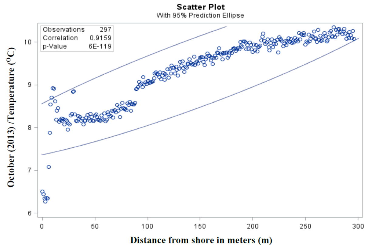
The next few figures present Pearson’s correlation results for the year 2013 as examples of the general correlation results. Figure 5 shows the negative correlations between August 2013 sediment temperature vs. distance from the shore. The August 2013 temperature declines until almost a 50 m distance is reached from the shore, then rises after 50 m for both locations. Thus, one can say that the water depth level after 50 m seems to become high enough to generate more cover for the sediment so that it receives more heat. It has been noted [6] that within a 0–50 m distance from the shore, flora (reeds, etc.) might affect the temperature. This is generally far enough from the shore that the sediment temperature is also seen to rise, meaning that more heat can be collected at this distance using sediment heat energy collection technologies. However, the water body type influences the distance from the shore depending on how shallow or deep the water body is. Particularly, according to our data, the best distance for sediment heat energy production is between 100 and 190 m from the shore, confirming the findings of Mäkiranta. However, this seems to depend on the month in which the data are collected, and in winter months there seems to be a constant increase in sediment temperature as the distance from the shore increases. In the upper section of Figure 5, the probability result is only at a 1% statistically significant level.
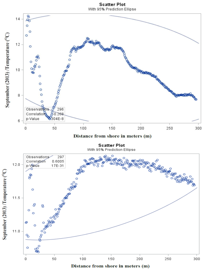
Figure 6 shows the September 2013 sediment temperature vs. distance correlations; the two locations have different results, where one is negative, and the other is positive. This can show how area specificity can influence this kind of correlation analysis and the sediment temperature patterns. Otherwise, the changes seen at different distances before and after 50 m are similar.
The difference between the results shown in the above two figures can be explained by the correlations between August and September 2013 sediment temperatures in the two locations. As noticed in further analysis, there are clear, statistically significant positive correlations at Ketunkatu. However, in Liito-oravankatu, the August and September 2013 sediment temperature show negative correlations. This can be explained by the specificity of both sediment temperature collection areas. Both locations had similar weather temperatures and are located in relatively close proximity. However, the shallowness of the water body and sediment soil characteristics can explain this to some extent and, as both locations are in the same water body, the sediment soil or sand characteristics are expected to be roughly similar. The October 2013 sediment temperature vs. distance shows positive correlations for both locations (Figure 7). However, the correlation shows much higher values for the Liito-oravankatu location. One can conclude that the location of the Liito-oravankatu installation seems to be deeper compared to the Ketunkatu location. This can be explained by the fact that, at the shore, the October temperature is lower in Ketunkatu than in Liito-oravankatu. In October in Finland, the air and water temperatures are somewhat colder due to the fact that winter is either approaching or has started already. Moreover, the weather change results in sediment temperature changes. Another factor is that, starting at the beginning of October, sediment heat uptake was started by the houses. Thus, the decline in sediment heat temperature at the beginning shore in the winter months could be due to the uptake of heat from sediment for household use.
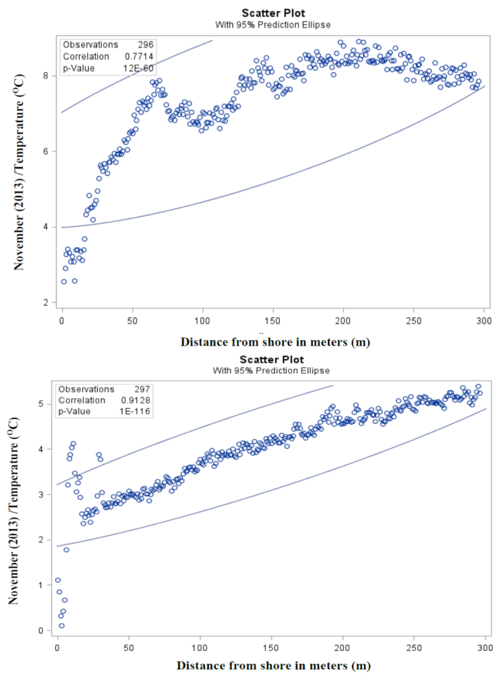
Further analysis showed positive correlations at Ketunkatu and negative correlations at Liito-oravankatu for sediment temperature between October and August 2013. In the location of Ketunkatu, as the October 2013 temperature increases, so does the August 2013 temperature. The opposite is true for the Liito-oravankatu location. This can be explained as the Liito-oravankatu installation is deeper, so the October 2013 temperature is lower than August 2013 at a distance of about 50 m. This confirms that the Liito-oravankatu installation location is deeper than Ketunkatu, in addition to the physical observation of the differences in these installation sites. However, other results show that both locations show positive correlations for October and September 2013 sediment temperatures. This is due to the fact that both months’ temperatures are somehow similar, at a colder temperature. However, at a specific depth location, the Ketunkatu sediment temperature is lower than that of Liito-oravankatu, which also confirms the depth difference between the two installation locations. Figure 8 shows positive correlations for November 2013 vs. distance for both locations. However, the Ketunkatu site show less linear correlation values compared to those of Liito-oravankatu. This is because the Liito-oravankatu installation is deeper than the Ketunkatu site and, in Ketunkatu, the depth of the water seems to be lower, until it is 50 m distance from the shore.
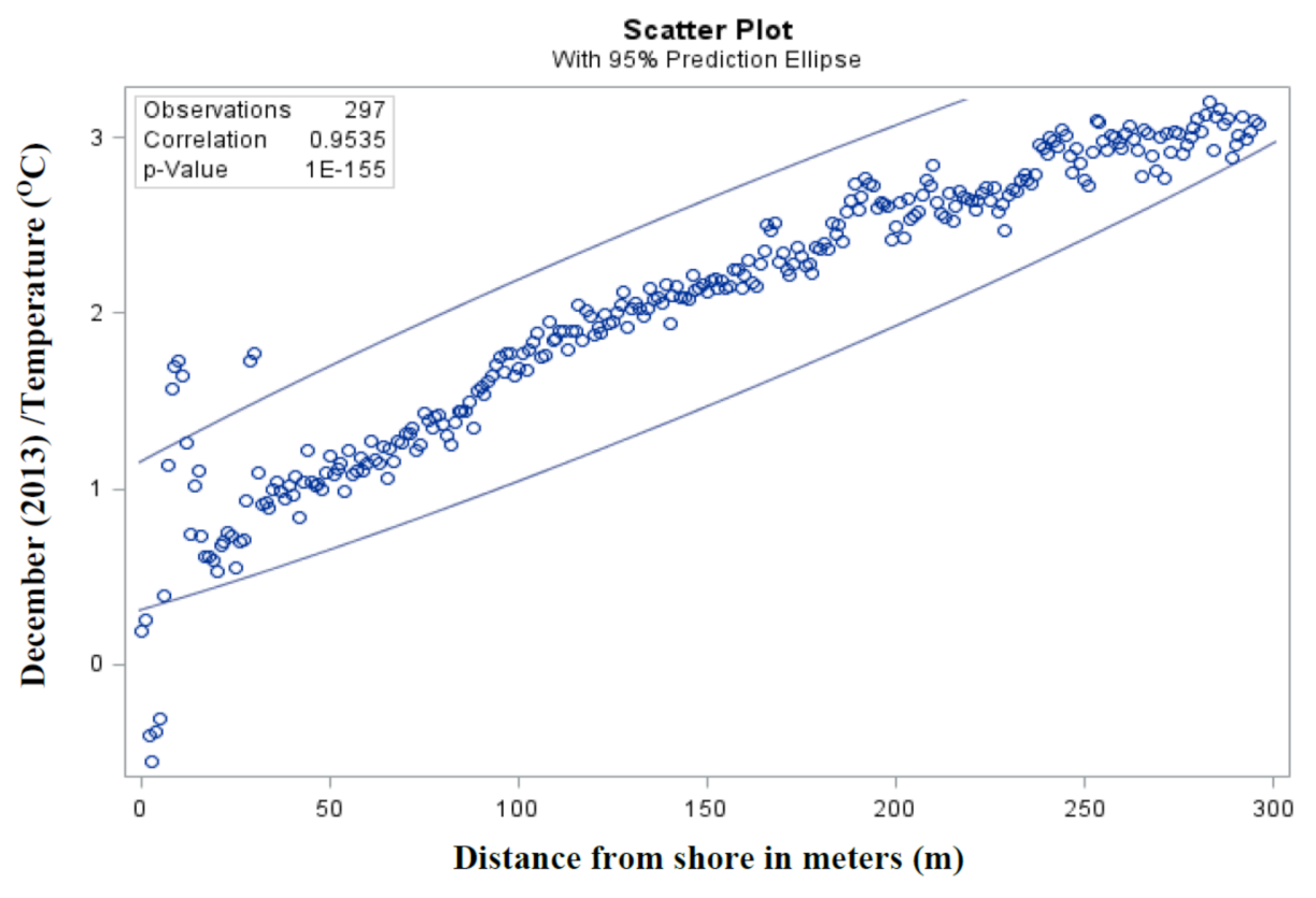
Other analyses show both sites’ Pearson’s correlations between November 2013 and August 2013 sediment temperatures, showing negative correlations. This is due to the fact that the different months have different weather temperatures, which affect the sediment heat energy or temperature. However, the Ketunkatu site correlations between November 2013 and August 2013 sediment temperatures are not statistically significant, which means that the presented results are not robust. However, we can accept the Liito-oravankatu site correlations for the same period as they are statistically significant. A similar observation in the Ketunkatu site sediment temperature correlations between November 2013 and September 2013 is not statistically significant, with a positive correlation. However, the Liito-oravankatu site correlations result is statistically significant between November 2013 and September 2013, and show that both the sediment temperatures in November and September were positive, even though the air temperature was negative most of the time. This is because the depth of this site is much deeper than that of the Ketunkatu site. December 2013 vs. distance correlations show similar results to those of November 2013 vs. distance (Figure 8), and Figure 9 shows the December 2013 vs. distance correlations results for both sites. Both sites show positive correlations, which are statistically significant.
November 2013 and October 2013 show statistically significant positive correlations. This is because both months’ temperatures were very similar; however, the variation in correlation values between the two sites reflects the differences in the site installation depth. There is a positive Pearson’s correlation between December 2013 vs. September, October, and November 2013, which is statistically significant. This is because these months have similar air temperatures and cause similar sediment heat temperatures. However, the correlations between December 2013 and August 2013 show a statistically significant negative correlation. This can be explained by the difference between the two months’ air temperature levels causing different sediment heat temperatures. Figure 10 shows the scatter plot matrix for all the correlation figures presented between the months of the year in 2013 and distance for both sites.

3.3. ARIMA Modeling Forecast

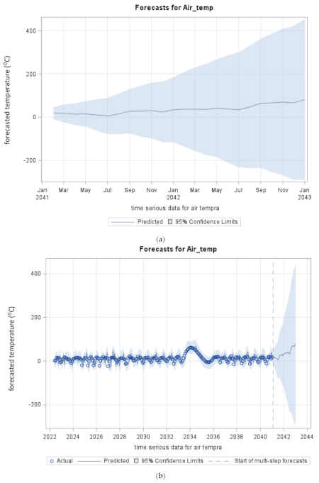
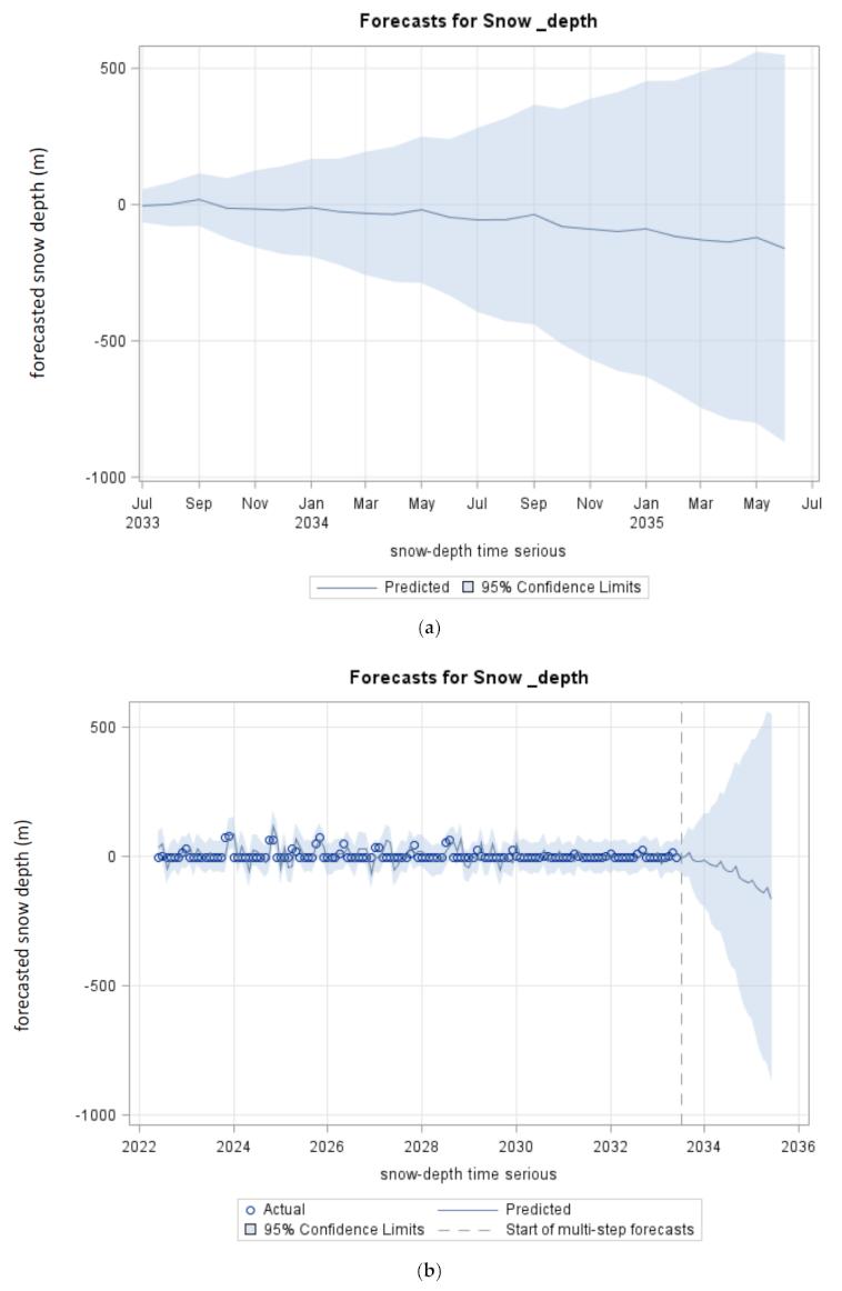
The forecasts presented here might not be representative because of a shortage of data. To conduct a true long-term forecasting (40 years of forecast) in any kind of modelling requires hundreds of years of data, which are not available in our area. However, the smaller dataset can represent the future situation to some degree. The forecast results presented in the current IPCC 2021 report [25] show approximately similar results. As can be seen in Figure 11, the air temperature is predicted to increase significantly after the year 2041, based on the collected data of mean air temperature between 1959 and 2019 from the Vaasa Airport weather station collected by the Finnish Meteorological Institute (FMI). The same weather station data predictions of snow depth (Figure 12) show a significant decline in 2033. The main cause of these change expectations is global warming. Consequently, these changes cause effects in water temperature, leading to changes in sediment temperature and its heat energy production. This means that the climate change effect could be advantageous for energy production is summer seasons. The snow cover is used as insulation for the sediment energy build-up, but when there is no snow cover in the future, the sediment energy in winter might decline. Furthermore, the warming of the winter weather may have different consequences in winter sediment energy production. To date, even if it is cold in winter, the sediment temperature has been positive, but this is expected to decline with snow melting caused by increases in winter temperature.
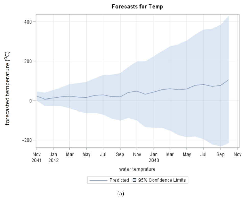
Our previous research found a positive correlation between air and water temperature, and a positive correlation between water temperature and sediment temperature with a 2-month lag. This suggests that air temperature affected by climate change will affect the water temperature, as well as the sediment temperature. Figure 13 shows how water temperature is expected to increase significantly after the year 2042. This forecast was conducted in a water body near the city of Vaasa at the Eteläinen Kaupunkiselkä 1 water sampling point by the Center for Economic Development, Transport and the Environment (ELY-keskus), and means that the water temperature will also change after the indicated air temperature increase in 2041. Moreover, it is expected this will lead to increases in sediment temperature, given that water temperature and sediment temperature have positive correlations after a 2-month lag. Consequently, energy production from sediment energy is expected to increase in the future, using the effects of climate change to its advantage, at least in the summer. However, in winter, this might be different.

3.4. Validations by Factor Analysis

The reliability and validity of quantitative research papers can be examined with conducting factor analysis, regarding construct validity [26]. Therefore, a factor analysis was conducted for both sediment energy sampling sites to validate the analyses that were conducted in this paper.

3.4.1. Validations by Factor Analysis for City of Vaasa at Suvilahti, Ketunkatu Site Data

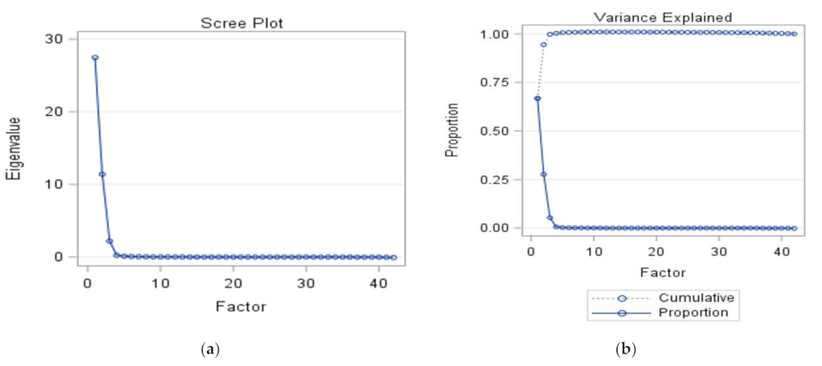
A total of 298 records were read, with 213 used and subject to significant tests (see Table 3). Four factors appear to explain most of the variability in the data, and these are presented in Table 3.
As can be seen in Figure 14, the first four factors account for most of the total data variability. The rest of the factors account only for a very small proportion of the variability and are likely to be unimportant. The first three factors have a variance (Eigenvalues) greater than 1, and one has a variance below 1. Therefore, four factors explain most of the variability in the data.
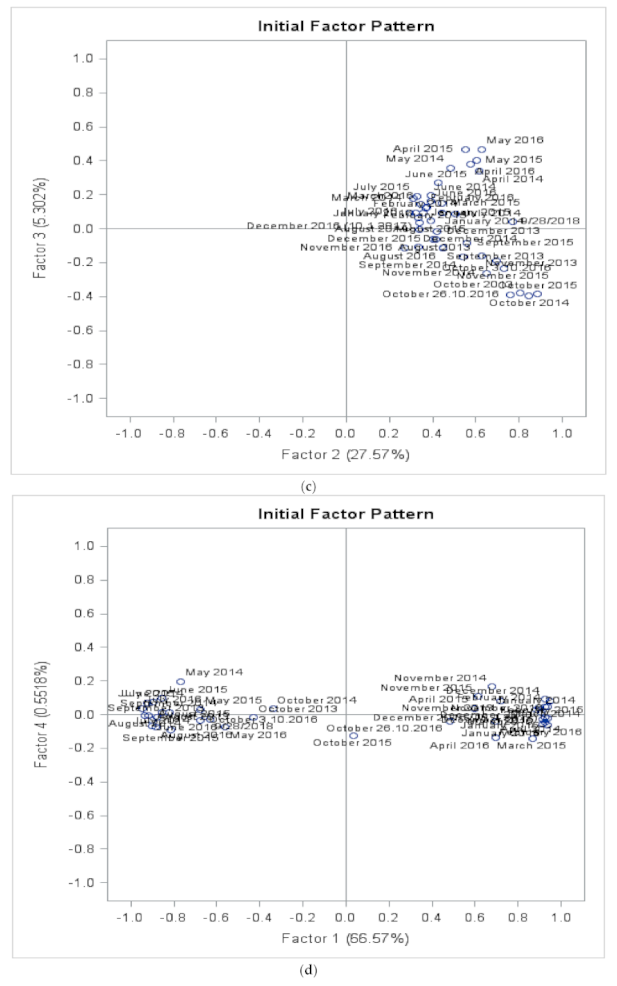
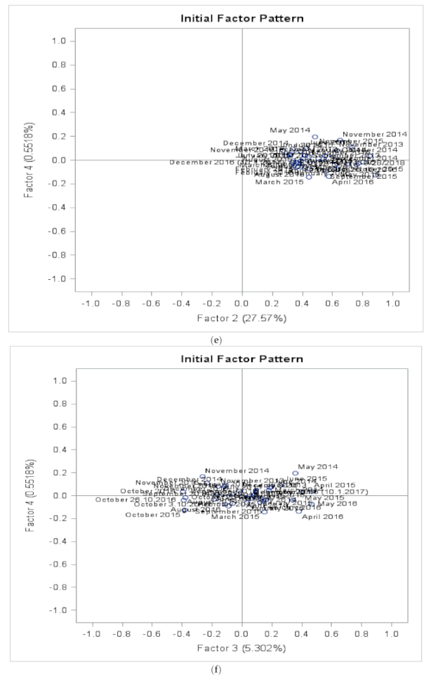
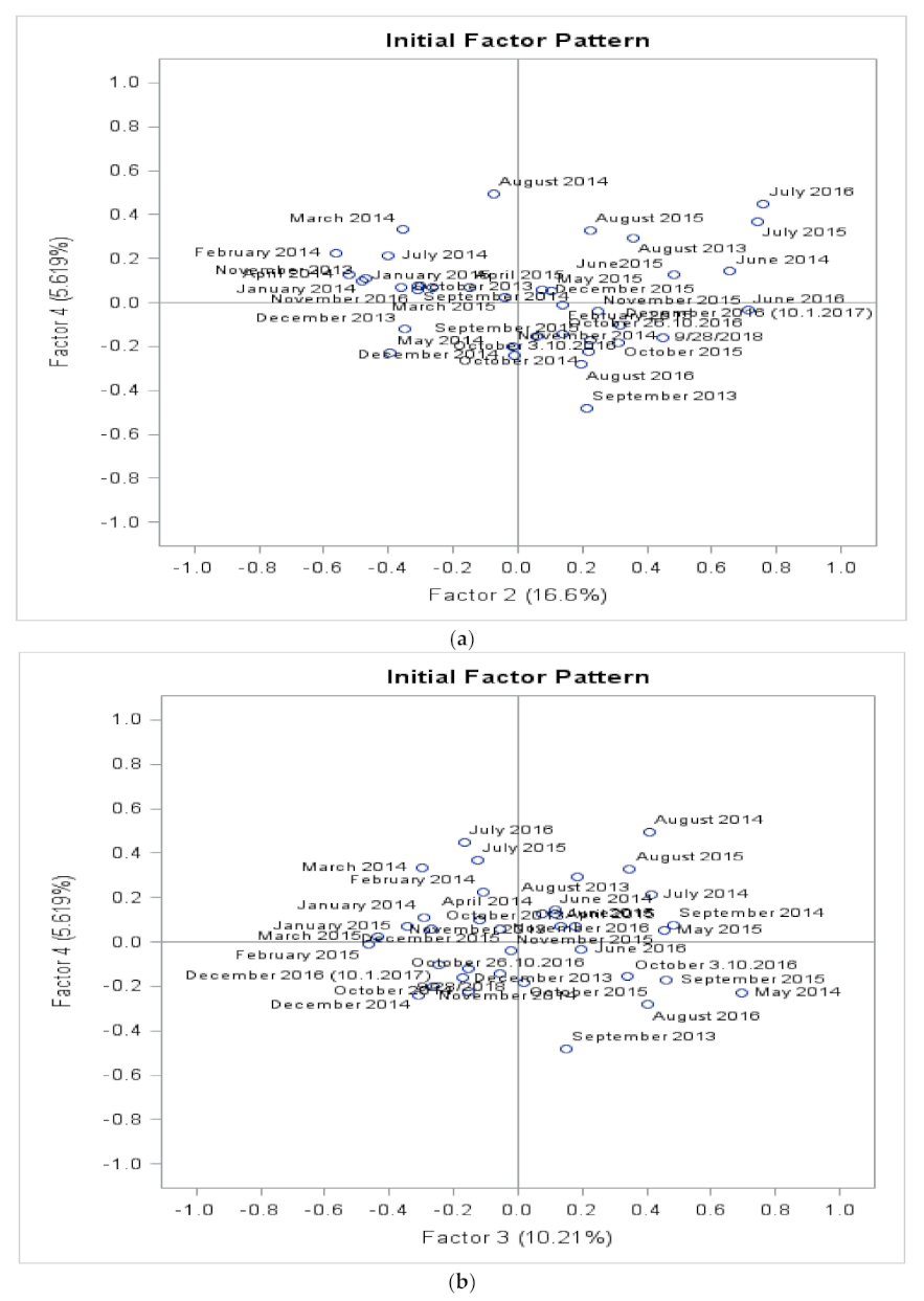
Figure 15 shows the score plots, where different factors are used in combination. As can be seen in factor 2 vs. factor 1, there is a cluster for summer and winter month data which explains most of the data pattern. Similar clusters were noticed in plots of factor 3 vs. factor 1 and factor 4 vs. factor 1. However, no outliers were found in the score plots. In addition, most of the data seem to be located in the middle area of the score plots. However, no clear trends were noticed except that the data of winter and summer months tend to cluster separately.
The Suvilahti, Ketunkatu site data may explain factors based on the data for Figure 15. Separation between the data of summer and winter months seems to be created by Factor 1. Factor 2 seems spread the data to the upper section of both winter and summer data separately, and/or all the data together. Factor 3 helps to bring all the data to the center of the plots, whereas factor 4 seems to cluster all the data together in separate seasons and/or without seasonal variations. The next factor analysis figures, do not seem clear enough and radiable due to the fact that they were automatically generated from SAS software. It was not possible to modify the figures to a better shape. However, they can show that the general result is representative enough.

3.4.2. Validations by Factor Analysis for the Suvilahti, Liito-Oravankatu Site Data

A total of 298 records were read, with 297 used and subject to significant tests (see Table 4). Five factors appear to explain most of the variability in the data. These are presented in Table 4.
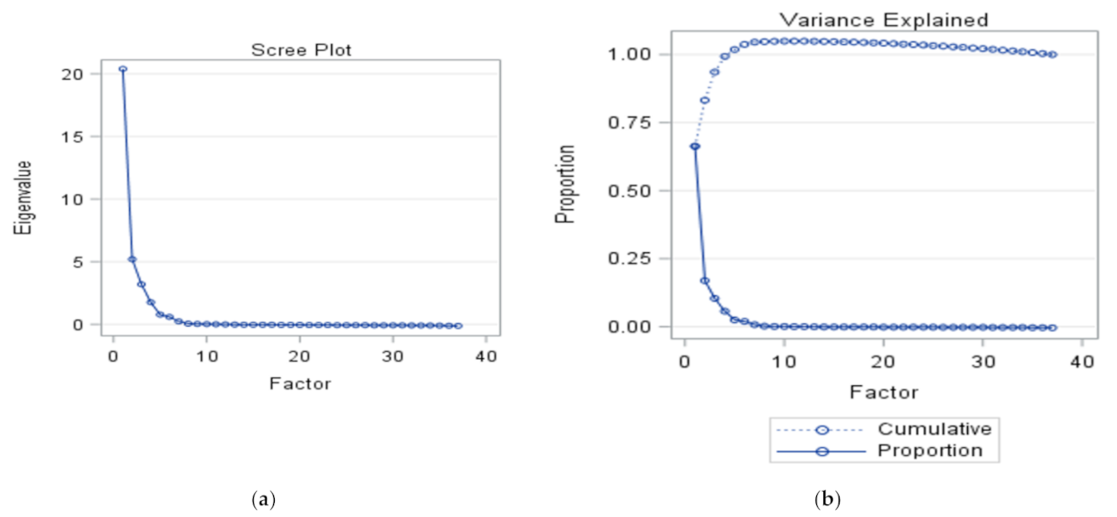
As can be seen in Figure 16, the first five factors account for most of the total variability in the data. The rest of the factors account for only a very small proportion of the variability and are likely to be unimportant. The first four factors show a variance (Eigenvalues) greater than 1, and one shows a variance below 1. Therefore, five factors explain most of the variability in the data (see Table 4).
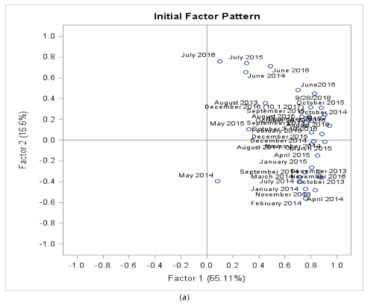
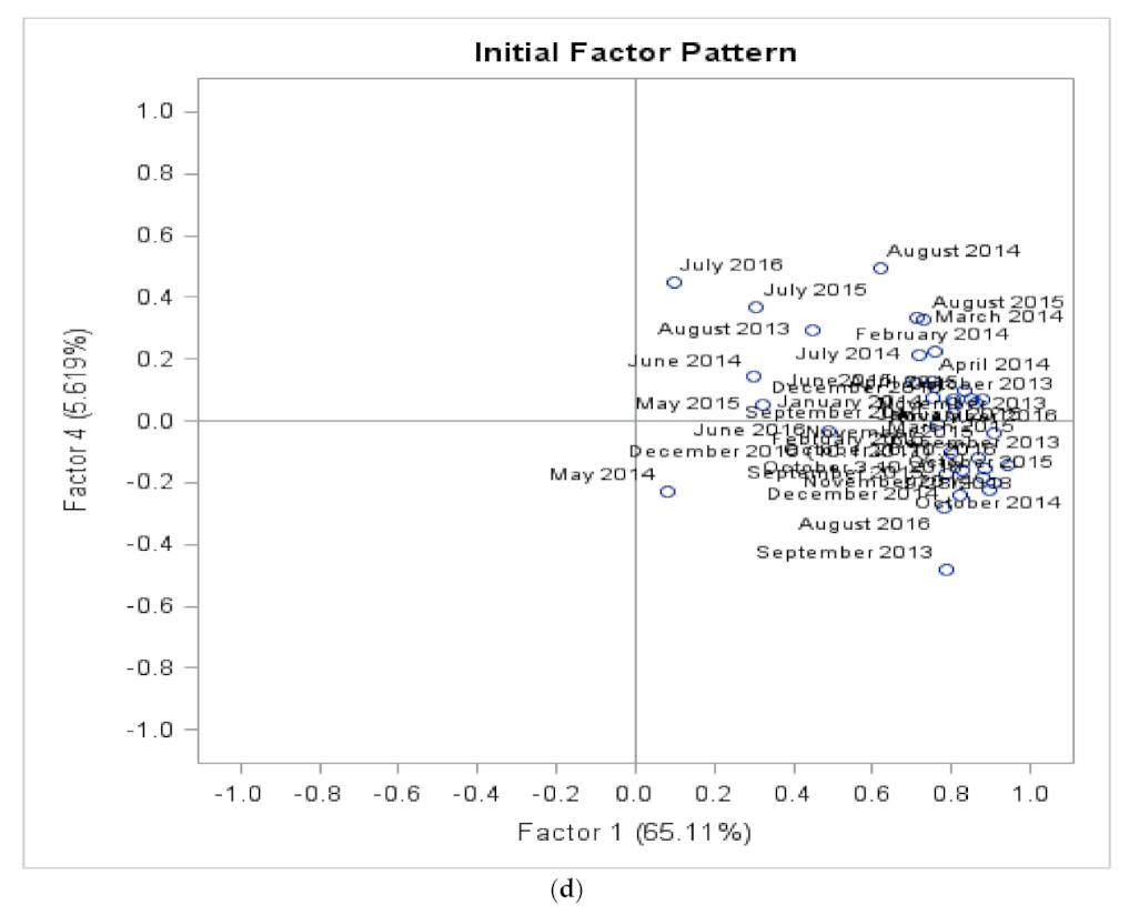
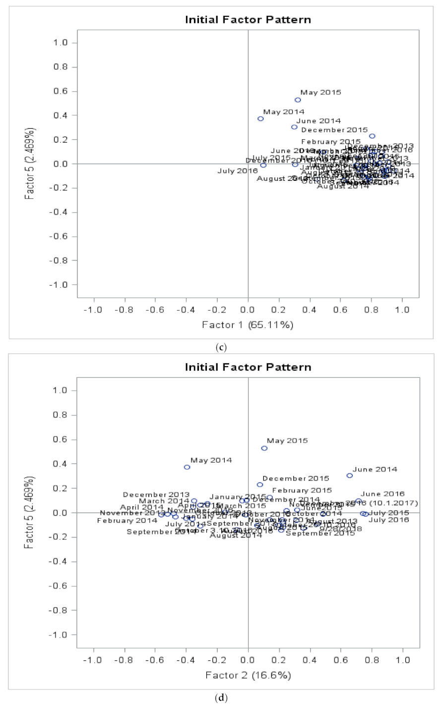
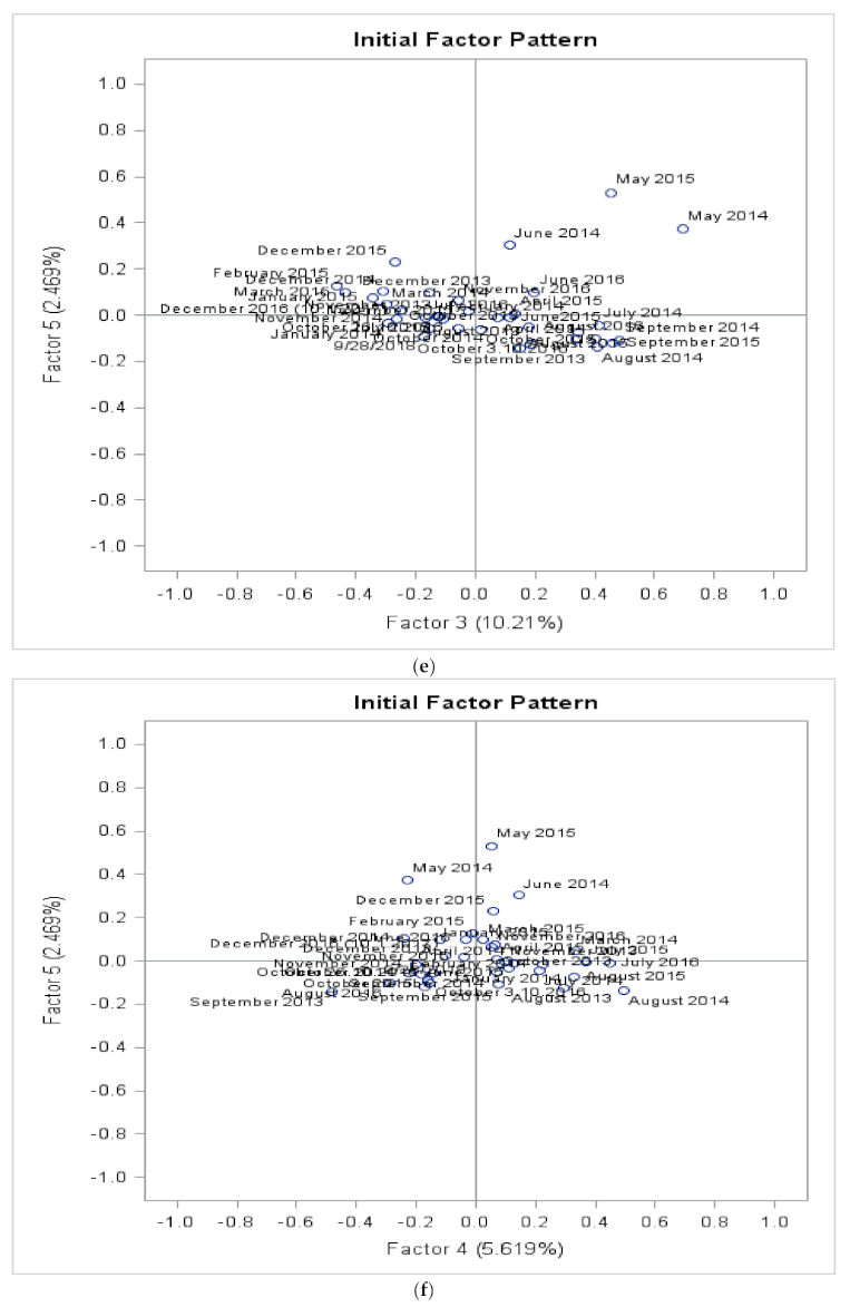
Comparing the score plots of Figure 17 and Figure 18 with those of Figure 15, there is a clear difference. In Figure 15, the winter and summer months cluster separately, but in the next two figures, both seasons’ data clusters are in one location, with the summer months’ data above the main section and the winter months’ data below. This can be explained by the differences in site specification between the analysis of the two sites.
The Suvilahti, Liito-oravankatu site data may explain factors based on the data for Figure 17 and Figure 18. Separation between the data of summer and winter months seems to be created by Factor 1. Factor 2 seems to spread the data to the upper and lower sections. Factor 3 helps to bring all the data to the center of the plots, whereas factor 4 seems to cluster all the data together in separate seasons and/or without seasonal variations. The spread of the data to the left and right sections seems to be caused by Factor 5. Most of the explanations for the factors are similar to those of Figure 15.
There are no clear outliers in Figure 17 and Figure 18. Factors 1 and 5 explain the proportion of most of the data. Some of the score plots below show that most of the data cluster is to the right and above the value of zero. The rest of the plots show a cluster near the center area. However, everything seems to be in a normal distribution pattern, depending on the month and the site specifications.
The analysis of sediment heat temperature data between 2013 and 2018 shows that most of the data were non-normal except for a few months. The result shows that this is site-specific while generalizing the results of summary statistics in terms of yearly patterns. This is probably due to the fact that the depth of installation for the two sites is different. The mean, median, and standard deviation variations seem to be yearly natural fluctuations.
A dependency analysis showed positive and negative Pearson’s correlation results. One of the main findings is that all the analyzed correlations between sediment temperature by months vs. distance were found to be statistically significant. The sediment temperature was higher on shore after sunny months. The negative correlation between sediment temperature and distance from shore can be explained by the fact that seabed sediment near the shore (smaller distance) had a higher temperature after sunny months. In addition to our findings, Kim and Cho [27] researched how seawater provides heat to the seabed at the intertidal zone (tidal flat) during the morning flood tide and gains heat from the seabed during the afternoon flood tide. Seawater heated by the atmosphere and seabed at the intertidal zone supplies heat to the sublittoral zone during spring, summer, and winter, but the opposite occurs in autumn. According to our findings, after 50 m, the sediment temperature rises in both locations. This was due to the water depth level after 50 m, which was seemingly enough to help the sediment generate more heat. One of the main findings was that distances between 100 and 190 m from the shore were best for sediment heat energy production in our sites. This result confirms our previous studies’ findings. Rinehimer and Thomson [28] observed that sediment–water heat fluxes are an important component of the heat budget, representing up to 20% of the incoming solar radiation and being larger than latent and sensible heat fluxes. Moreover, Guarini and Blanchard [29] modelled the spatio–temporal dynamics of mud surface temperatures. Comparisons at different periods between measured data series and simulations clearly establish the reliability of the model, thus allowing for extrapolations over time and space [29].
ARIMA modeling forecasts might not present the exact truth, due to a shortage of data in our area; hundreds of datapoints are required to forecast for about 40 years. This means that the generalizability of the forecast is limited by this requirement in modeling. However, the result of the forecast was found to be similar to IPCC (2021) [25] forecasts, which are representative enough to show that what is expected in a local area may be expected worldwide. Future air and water temperature rises are expected to benefit sediment heat energy production, at least in summertime, with a 2-month lag. In winter, with the expectations of a decline in snowfall in the future, there may be a decline the sediment heat-energy production. This is due to ice and snow cover on the water body acting as an insulation layer, assisting in sediment heat production during winter. On the other hand, when there is no more snow cover in water bodies, it is expected that winter sediment heat-energy production will decline. This suggests that the sediment heat-energy only benefits from weather change caused by climate change in summer. This helps to increase the significance of our results by building on the theoretical and practical implications that climate change can be implemented by using the temperature increase effect in air and water temperature to increase sediment heat energy production.
Validation by factor analysis shows all the data were clustered and no particular outliers were noticed. Climate change has a clear effect on air and water temperature changes at present, as reported in the IPCC 2021 report [25]. This means that finding ways to adapt, combat, and mitigate climate change is an essential way forward. The main finding of this study is that renewable sediment heat energy uses climate change to its advantage, which could be one solution to using climate change to our advantage. The simulation results of Fang et al. indicated that the influence of water temperature on sediment temperature is very strong, especially in deep lakes [30]. Thus, our result findings that climate change causes water temperature increases, which is advantageous for sediment heat energy, at least in summertime, is supported by Fang et al. Further research and data collection in sediment heat energy production sites is recommended to establish a more compressive theory, which can be generalized to all water body types.

4. Conclusions

Our conclusion, based on a summary of statistics, is that the pattern was site-specific and depended on installation depth. This was also confirmed during dependency analysis. In addition, based on mean, median, and standard deviations, it was concluded that the data show annual natural fluctuations.
ARIMA modeling shows some limitations of our study, but is representative enough to suggest that air and water temperatures are expected to rise and snow fall is expected to decline in the future. Sediment heat energy production uses the climate change effect to its advantage, especially in the summer. There are expectations or forecasts of air and water temperature increases in the future, leading to an increase in sediment temperature with a 2-month time lag. Therefore, the air temperature and solar irradiance increases caused by the climate change effect are expected to increase water temperature. An increase in water temperature causes further increases in sediment temperatures in summer. In winter, ice and snow cover used to act as an insulation for sediment heat energy production or sediment temperature. However, due to a decline in snow cover in winter, the cold temperature of the winter air might reduce the sediment heat, especially in shallow shores. Thus, this could lead to a decline in heat-energy production from sediment in winter. However, we conclude that, in summer, sediment heat energy production has, and will, continue to use the climate change effect to its own advantage.
Dependency analysis shows negative correlations between sediment temperature per month vs. distance from shore in sunny months and a positive correlation in winter months. In addition, the sediment temperature seems to build up after a 30–50 m distance from the shore, depending on the shallowness of the water body. In winter months (starting from October), the decline in 30–50 m sediment heat temperature could occur due to the heat uptake for household use. Notably, our data show that the best distance for sediment heat energy production in summer is between 100 and 190 m (sediment temperature record distance from shore), confirming the previous studies of our research group. However, this seems to depend on the month in which the data are collected. In winter months there seems to be a constant increase in sediment temperature as the distance from the shore increases. Generally, the findings presented in this paper offer new insight into the benefits of climate change effects for renewable energy production, and can, thus, be used to combat climate change more efficiently. Therefore, this provides some good news about climate change effects, even though its disadvantages are much more significant.
Validations by factor analysis show that data analysis was performed correctly. An additional point that was noticed was that, in other analyses, the turbidity of water bodies is expected to increase in the far future. This means that, as turbidity increases, this will lead to an increase in the absorbance of solar irradiance by the water body. This leads to an increase in water temperature and is further expected to increase the sediment heat temperature. There is a clear connection between limnology and sediment heat energy productions.

Author Contributions

Conceptualization, N.G. and A.M.; methodology, N.G. and A.M.; software, N.G.; validation, N.G. and A.M.; formal analysis, N.G. and A.M.; investigation, A.M.; writing—original draft preparation, N.G.; writing—review and editing, A.M., N.G., X.L. and E.H. All authors have read and agreed to the published version of the manuscript.

Funding

The researcher N.G. received funding from E.E. and G.E. foundation during work on this article. The University of Vaasa is acknowledged for providing a suitable working environment, researchers, resources, and costs coverage.

Institutional Review Board Statement

Not applicable.

Informed Consent Statement

Not applicable.

Data Availability Statement

The data presented in this study are available on request from the corresponding author. The data are not publicly available as this research is ongoing and contains the university’s own research results.

Acknowledgments

We acknowledge the E.E. and G.E. foundation for providing a doctoral student grant to N.G. during the period of writing this article. We also want to thank the University of Vaasa for their support during the research period. We would also like to acknowledge N.R. for proofreading and editing.

Conflicts of Interest

The authors declare no conflict of interest.

Abbreviations

ARIMAAutoregression Integrated Moving Average
DTSDistributed Temperature Sensing
FMIFinnish Meteorological Institute
ELY-keskusCenter for Economic Development, Transport, and the Environment
IPCCIntergovernmental Panel on Climate Change
Pt100sThe most common Platinum resistance thermometer
SASStatistical Analysis Software (Enterprise Guide 7.1)

References

  1. Hiltunen, E.; Martinkauppi, J.B.; Mäkiranta, A.; Rinta-Luoma, J.; Syrjälä, T. Seasonal temperature variation in heat collection liquid used in renewable, carbon-free heat production from urban and rural water areas. Agron. Res. 2015, 13, 485–493. [Google Scholar]
  2. Likens, G.E.; Johnson, N.M. Measurement and analysis of the annual heat budget for the sediment in two Wisconsin lakes. Limnol. Oceanogr. 1969, 14, 115–135. [Google Scholar] [CrossRef]
  3. Oceanography 101 (Miracosta). (15 February 2021). Available online: https://geo.libretexts.org/@go/page/9666 (accessed on 18 July 2021).
  4. Savola, A. Fluid Flow Modeling Inside Heat Collection Pipes with Finite Element Method. Master’s thesis, University of Vaasa, Vaasa, Finland, 2012. [Google Scholar]
  5. Mäkiranta, A. Distributed Temperature Sensing Method–Usability in Asphalt and Sediment Heat Measurement. Master’s thesis, University of Vaasa, Vaasa, Finland, 2013. [Google Scholar]
  6. Ukil, A.; Braendle, H.; Krippner, P. Distributed temperature sensing: Review of technology and applications. IEEE Sens. J. 2012, 12, 885–892. [Google Scholar] [CrossRef] [Green Version]
  7. Wilcock, W.S.D.; Kauffman, P.C. Development of a seawater battery for deep-water applications. J. Power Sources 1997, 66, 71–75. [Google Scholar] [CrossRef]
  8. Wang, Y.; Liu, D.; Richard, P.; Li, X. A geochemical record of environmental changes in sediments from Sishili Bay, northern Yellow Sea, China: Anthropogenic influence on organic matter sources and composition over the last 100 years. Mar. Pollut. Bull. 2013, 77, 227–236. [Google Scholar] [CrossRef]
  9. Reimers, C.R.; Tender, L.M.; Fertig, S.; Wang, W. Harvesting energy from the marine sediment-water interface. Environ. Sci. Technol. 2001, 35, 192–195. [Google Scholar] [CrossRef] [PubMed]
  10. Hiltunen, E.; Martinkauppi, J.B.; Zhu, L.; Mäkiranta, A.; Lieskoski, M.; Rinta-Luoma, J. Renewable, carbon-free heat production from urban and rural water areas. J. Clean. Prod. 2015, 153, 379–404. [Google Scholar] [CrossRef]
  11. Mäkiranta, A.; Martinkauppi, J.B.; Hiltunen, E. Seabed sediment—A natural seasonal heat storage feasibility study. Agron. Res. 2017, 15 (Suppl. S1), 1101–1106. [Google Scholar]
  12. Mäkiranta, A.; Martinkauppi, J.B.; Hiltunen, E. Correlation between temperature of air, heat carrier liquid and seabed sediment in renewable low energy network. Agron. Res. 2016, 14 (Suppl. S1), 1191–1199. [Google Scholar]
  13. Mäkiranta, A.; Martinkauppi, B.; Hiltunen, E.; Lieskoski, M. Seabed sediment as an annually renewable heat source. Appl. Sci. 2018, 8, 290. [Google Scholar] [CrossRef] [Green Version]
  14. Sebok, E.; Müller, S. The effect of sediment thermal conductivity on vertical groundwater flux estimates. Hydrol. Earth Syst. Sci. 2019, 23, 3305–3317. [Google Scholar] [CrossRef] [Green Version]
  15. Goto, S.; Yamano, M.; Morita, S.; Kanamatsu, T.; Hachikubo, A.; Kataoka, S.; Tanahashi, M.; Matsumoto, R. Physical and thermal properties of mud-dominant sediment from the Joetsu Basin in the eastern margin of the Japan Sea. Mar. Geophys. Res. 2017, 38, 393–407. [Google Scholar] [CrossRef] [Green Version]
  16. Guo, Y.; Ma, J. Temperature Rise of Seawater Simulation under the Influence of Sediment-Water Heat Exchange. Water 2018, 10, 656. [Google Scholar] [CrossRef] [Green Version]
  17. Golosov, S.; Kirillin, G. A parameterized model of heat storage by lake sediments. In Environmental Modeling and Software; Elsevier: Amsterdam, The Netherlands, 2010; Volume 25, pp. 793–801. [Google Scholar] [CrossRef]
  18. Pivato, M.; Carniello, L.; Gardner, J.; Silvestri, S.; Marani, M. Water and sediment temperature dynamics in shallow tidal environments: The role of the heat flux at the sediment-water interface. Adv. Water Resour. 2018, 113, 126–140. [Google Scholar] [CrossRef]
  19. Hamilton, D.P.; Magee, M.R.; Wu, C.H.; Kratz, T.K. Ice cover and thermal regime in a dimictic seepage lake under climate change. Inland Waters 2018, 8, 381–398. [Google Scholar] [CrossRef]
  20. Ellis, C.R.; Stefan, H.G.; Gu, R. Water temperature dynamics and heat transfer beneath the ice cover of a lake. Limnol. Oceanogr. 1991, 36, 324–335. [Google Scholar] [CrossRef]
  21. Smith, P.N. Observations and simulations of water-sediment heat exchange in a shallow coastal lagoon. Estuaries 2002, 25, 483–487. [Google Scholar] [CrossRef]
  22. Tsay, T.-K.; Ruggaber, G.J.; Effler, S.W.; Driscoll, C.T. Thermal Stratification modeling of lakes with sediment heat flux. J. Hydraul. Eng. 1992, 118, 407–419. [Google Scholar] [CrossRef]
  23. Meyers, L.S.; Gamst, G.; Guarino, A.J. Data Analysis Using SAS Enterprise Guide; Cambridge University Press: Cambridge, UK, 2009; ISBN -13. [Google Scholar]
  24. Dytham, C. Choosing and Using Statistics—A Biologist’s Guide, 3rd ed.; John Wiley & Sons: Hoboken, NJ, USA, 2011; ISBN 978-1-4443-2843-1. [Google Scholar]
  25. IPCC. Climate Change 2021: The Physical Science Basis. In Proceedings of the Contribution of Working Group— I to the Sixth Assessment Report of the Intergovernmental Panel on Climate Change (IPCC AR6 WGI), 2021. Available online: https://www.ipcc (accessed on 31 July 2021).
  26. Drucker-Godard, C.; Ehlinger, S.; Grenier, C. Validity and Reliability. In Doing Management Research; SAGE Publication Ltd.: London, UK, 2011; pp. 196–220. [Google Scholar] [CrossRef]
  27. Kim, T.W.; Cho, Y.K. Calculation of heat flux in a macrotidal flat using FVCOM. J. Geophys. Res. Ocean. 2011, 116, 869–881. [Google Scholar] [CrossRef] [Green Version]
  28. Rinehimer, J.P.; Thomson, J.T. Observations and modeling of heat fluxes on tidal flats. J. Geophys. Res. Ocean. 2014, 119, 133–146. [Google Scholar] [CrossRef]
  29. Guarini, J.M.; Blanchard, G.F.; Gros, P.; Harrison, S.J. Modelling the mud surface temperature on intertidal flats to investigate the spatio-temporal dynamics of the benthic microalgal photosynthetic capacity. Mar. Ecol. Prog. Ser. 1997, 153, 25–36. [Google Scholar] [CrossRef]
  30. Fang, X.; Stefan, H.G. Temperature variability in lake sediments. Water Resour. Res. 1997, 34, 717–729. [Google Scholar] [CrossRef]
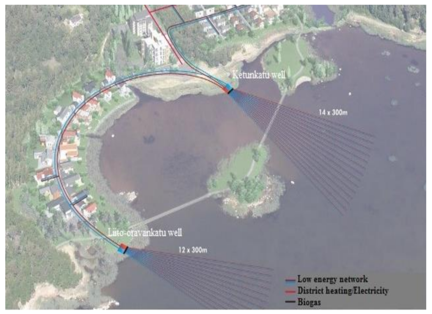
Figure 1. Suvilahti low-energy network sharing heating and cooling for 42 houses (Vaasan Ekolämpö Oy).
Energies 15 00435 g001
Figure 2. Profile of a Refla heat-collection pipe (A. Mäkiranta 2013).
Energies 15 00435 g002
Figure 3. Sensornet Oryx DTS device that can be used even in outdoor conditions.
Energies 15 00435 g003
Figure 4. Summary of statistical data for sediment temperature in degrees Celsius (°C), summarized for whole depths: mean, standard deviation, and median at Suvilahti, Ketunkatu, in the city of Vaasa.
Energies 15 00435 g004
Figure 5. Plot showing Pearson’s correlations between August 2013 temperature and distance at Suvilahti, in the city of Vaasa. Ketunkatu (above) and Liito-oravankatu (below). The meaning of p-value = 14E−43 = 14 × 10 −43 (below).
Energies 15 00435 g005
Figure 6. Plot showing Pearson’s correlations between September 2013 temperature and distance at Suvilahti, in the city of Vaasa. Ketunkatu (above) and Liito-oravankatu (below). The meaning of p-value = 304E−8 = 304 × 10−8 (above). The meaning of p-value = 17E−31 = 17 × 10−31 (below).
Energies 15 00435 g006
Figure 7. Plot showing Pearson’s correlation between October 2013 temperature and distance at Suvilahti in the city of Vaasa. Ketunkatu (above) and Liito-oravankatu (below). The meaning of p-value = 674E−8 = 674 × 10−8 (above). The meaning of p-value = 6E−119 = 6 × 10−119 (below).
Energies 15 00435 g007aEnergies 15 00435 g007b
Figure 8. Plot showing Pearson’s correlation between November 2013 temperature and distances at Suvilahti in the city of Vaasa. Ketunkatu (above) and Liito-oravankatu (below). The meaning of p-value = 12E−60 = 12 × 10−60 (above). The meaning of p-value = 1E−116 = 1 × 10−116 (below).
Energies 15 00435 g008
Figure 9. Plot showing Pearson’s correlation between December 2013 temperature and distance at the city of Vaasa, Suvilahti. Ketunkatu (above) and Liito-oravankatu (below). The meaning of p-value = 17E−71 = 17 × 10−71 (above). The meaning of p-value = 1E−155 = 1 × 10−155 (below).
Energies 15 00435 g009aEnergies 15 00435 g009b
Figure 10. Scatter plot matrix showing the months of the year in 2013 vs. distance for both sites at Suvilahti in the city of Vaasa. Ketunkatu (left) and Liito-oravankatu (right).
Energies 15 00435 g010
Figure 11. ARIMA analysis for the air temperature forecast over time from the Vaasa airport weather station. In the figure -200 = minus 200. (a) shows temperature forecast from 2041 to 2043. (b) shows forecast in air temperature from 2022 to 2044.
Energies 15 00435 g011
Figure 12. ARIMA analysis for the snow-depth forecast over time from the Vaasa airport weather station. In the figure − 500 or −1000 = minus 500 or minus 1000. (a) shows forecast in snow depth since 2033 up to 2035. (b) shows forecast in snow depth from 2022 to 2036.
Energies 15 00435 g012
Figure 13. ARIMA analysis for the water temperature forecast over time at a different location than the sediment energy location (Eteläinen Kaupunkiselkä 1) near the city of Vaasa. In the figure – 200 = minus 200. (a) shows forecast in water temperature 2041 up to 2043. (b) shows forecast in water temperature from 2022 to 2044.
Energies 15 00435 g013aEnergies 15 00435 g013b
Figure 14. Scree plot (a) Eigenvalue vs. factors and (b) proportion vs. factors: four factors are retained by the PROPORTION criterion.
Energies 15 00435 g014
Figure 15. Six score plots built for four factor combinations at the Ketunkatu site. (a) Factor 2 vs. Factor 1. (b) Factor 3 vs. Factor 1. (c) Factor 3 vs. Factor 2. (d) Factor 4 vs. Factor 1. (e) Factor 4 vs. Factor 2. (f) Factor 4 vs. Factor 3.
Energies 15 00435 g015aEnergies 15 00435 g015bEnergies 15 00435 g015c
Figure 16. Scree plots (a) Eigenvalue vs. factors and (b) proportion vs. factor: five factors are retained by the PROPORTION criterion.
Energies 15 00435 g016
Figure 17. Four score plots built for five factor combinations at the Liito-oravankatu site. (a) Factor 2 vs. Factor 1. (b) Factor 3 vs. Factor 1. (c) Factor 3 vs. Factor 2. (d) Factor 4 vs. Factor 1.
Energies 15 00435 g017aEnergies 15 00435 g017bEnergies 15 00435 g017c
Figure 18. Six score plots built for five factor combinations at the Liito-oravankatu site. (a) Factor 4 vs. Factor 2. (b) Factor 4 vs. Factor 3. (c) Factor 5 vs. Factor 1. (d) Factor 5 vs. Factor 2. (e) Factor 5 vs. Factor 3. (f) Factor 5 vs. Factor 4.4. Discussion.
Energies 15 00435 g018aEnergies 15 00435 g018bEnergies 15 00435 g018c
Table 1. Pearson’s correlations analysis between different months and increment of depth/distance at Suvilahti, Ketunkatu in the city of Vaasa. The first row shows Pearson’s correlation results, the second row shows statistical significance, and the third row shows the number of samples in each analysis.
Pearson’s Correlation for Month Temperature vs. Distance
Distance Distance Distance Distance Distance Distance Distance
distance114 January0.8350214 July−0.2375715 January0.8379815 July−0.3658416 January0.7847316 July−0.40112
<0.0001<0.0001<0.0001<0.0001<0.0001<0.0001
297297297297297297297
13 August−0.0639814 February0.8585814 August−0.473515 February0.8478215 August−0.4501316 February0.82599August−0.36077
0.2717<0.0001<0.0001<0.0001<0.0001<0.0001<0.0001
297297297297297297297
13 September−0.2675114 March0.8826914 September−0.3378415 March0.86115 September−0.351716 March0.855453 October 2016−0.06442
<0.0001<0.0001<0.0001<0.0001<0.0001<0.00010.2684
296297297297297297297
13 October0.258314 April0.8899714 October0.0731114 April0.9226815 October0.2326316 April0.7869526 October 20160.56589
<0.0001<0.00010.209<0.0001<0.0001<0.0001<0.0001
296297297297297214297
13 November0.7714213 May0.3660614 November0.6766415 May0.60669November 150.6613116 May0.5890716 November0.78826
<0.0001<0.0001<0.0001<0.0001<0.0001<0.0001<0.0001
296297297297297297297
13 December0.8112614 June−0.2191214 December0.7934515 June−0.0669715 December0.7892116 June−0.18148December 2016 (10 January 2017)0.83927
<0.00010.0001<0.00010.2499<0.00010.0017<0.0001
296297297297297297297
28 September 20180.35938
<0.0001
297
Table 2. Pearson’s correlations analysis between different months of years and increment of depth/distance at Suvilahti, Liito-oravankatu, in the city of Vaasa. The first row shows Pearson’s correlation results, the second row shows statistical significance, and the third row shows the number of samples in each analysis.
Pearson’s Correlation for Month Temperature vs. Distance
Distance DistanceDistance Distance Distance Distance Distance
distance114 January0.8386114 July0.6652515 January0.9415615 July−0.6159816 June0.62211
<0.0001<0.0001<0.0001<0.0001<0.0001
297297297297297297
13 August−0.6856414 February0.9166114 August−0.9137815 February0.9528315 August−0.3867916 July−0.88149
<0.0001<0.0001<0.0001<0.0001<0.0001<0.0001
297297297297297297
13 September0.6005314 March0.957114 September0.5616215 March0.9423415 September0.7082816 August0.66973
<0.0001<0.0001<0.0001<0.0001<0.0001<0.0001
297297297297297297
13 October0.915914 April0.9386214 October0.9278415 April0.9670315 October0.936963 October 20160.9117
<0.0001<0.0001<0.0001<0.0001<0.0001<0.0001
297297297297297297
13 November0.9127614 May0.7818114 November0.9528215 May0.8709415 November0.9506726 October 20160.94707
<0.0001<0.0001<0.0001<0.0001<0.0001<0.0001
297297297297297297
13 December0.9534714 June−0.6746814 December0.9650215 June0.8070515 December0.9656816 November0.95512
<0.0001<0.0001<0.0001<0.0001<0.0001<0.0001
297297297297297297
December 2016 (10 January 2017)0.96501
<0.0001
297
28 September 20180.89186
<0.0001
297
Table 3. Analysis information for factor analysis at the Ketunkatu site.
Input Data TypeRaw Data
Number of Records Read298
Number of Records Used213
N for Significance Tests213
Variance Explained by Each Factor
Factor 1Factor 2Factor 3Factor 4
27.47999511.3823382.1886760.227792
Table 4. The table presenting the analysis info for facto analysis at site Liito-oravankatu.
Input Data TypeRaw Data
Number of Records Read298
Number of Records Used297
N for Significance Tests297
Variance Explained by Each Factor
Factor 1Factor 2Factor 3Factor 4Factor 5
20.3909205.1981813.1960841.7597240.773356
Publisher’s Note: MDPI stays neutral with regard to jurisdictional claims in published maps and institutional affiliations.