
XGBoost-Based Day-Ahead Load Forecasting Algorithm Considering Behind-the-Meter Solar PV Generation


Department of Electrical Engineering, Soongsil University, Seoul 06978, Korea
*
Author to whom correspondence should be addressed.
Energies 2022, 15(1), 128; https://doi.org/10.3390/en15010128
Submission received: 24 November 2021
/
Revised: 13 December 2021
/
Accepted: 21 December 2021
/
Published: 24 December 2021
(This article belongs to the Special Issue Short-Term Load Forecasting 2021)
Abstract
:With the rapid expansion of renewable energy, the penetration rate of behind-the-meter (BTM) solar photovoltaic (PV) generators is increasing in South Korea. The BTM solar PV generation is not metered in real-time, distorts the electric load and increases the errors of load forecasting. In order to overcome the problems caused by the impact of BTM solar PV generation, an extreme gradient boosting (XGBoost) load forecasting algorithm is proposed. The capacity of the BTM solar PV generators is estimated based on an investigation of the deviation of load using a grid search. The influence of external factors was considered by using the fluctuation of the load used by lighting appliances and data filtering based on base temperature, as a result, the capacity of the BTM solar PV generators is accurately estimated. The distortion of electric load is eliminated by the reconstituted load method that adds the estimated BTM solar PV generation to the electric load, and the load forecasting is conducted using the XGBoost model. Case studies are performed to demonstrate the accuracy of prediction for the proposed method. The accuracy of the proposed algorithm was improved by 21% and 29% in 2019 and 2020, respectively, compared with the MAPE of the LSTM model that does not reflect the impact of BTM solar PV.
1. Introduction
Day-ahead load forecasting is one of the main tasks for power system operation and planning [1]. Accurate load forecasting is essential for stable power system operation [2,3]. Renewable energy is the fastest-growing energy source in South Korea. Some of the renewable energy sources are located behind the electric meter, so the system operator cannot monitor behind-the-meter (BTM) generators in real-time. The electric load used for the operation of the power system in South Korea refers to the amount of metered generation at the generator output terminal [4]. Since the amount of BTM generation is not measured in real time, the electrical load is the actual power consumption minus the amount of BTM generation. At the end of 2019, the total capacity of solar PV generators in South Korea was 10,505 MW. The metered solar PV generator capacity is only 3242 MW [5]. So far, the management system for solar power generators is not unified or systematic in South Korea, and some solar PV generators are not included in the statistics. Therefore, the actual installed capacity of BTM solar PV generators is estimated to be much larger. With the increase in BTM solar PV generators, load distortion is increasing, and this is a major cause of increasing uncertainty in load forecasting.
Since electric load is highly related to various factors, such as the weather, holidays and events, accurate load forecasting is a challenging problem, and related research has been receiving a lot of attention [6]. Load forecasting techniques can be divided into statistical methods and machine learning methods. Statistical methods can reflect the time series characteristics [7,8,9,10,11]. Statistical methods have limitations in load forecasting nonlinearly changing electrical load due to various factors. In order to overcome these limitations, the proposed method employs machine learning techniques that can reflect nonlinearity. Representative machine learning methods include neural network (NN), decision tree and support vector regression (SVR), which show superior performance compared with the statistical method [2,12,13,14,15,16,17,18]. In recent years, more attention has been devoted to analyzing the impact of BTM solar PV generators on electric load [18,19,20,21,22,23,24,25,26]. Li et al. [20] presented a two-stage decoupled estimation for extracting PV generation from net load. Bu et al. [21] proposed a data-driven approach on net load disaggregation using clustering and game theory. Li et al. [22] proposed a method of estimating the capacity of BTM solar PV generators by extracting features from the discrepancy between two different net load curves under heterogeneous weather conditions. This method does not reflect the impact of weather factors or the load used by lighting appliances. Shaker et al. [23,24] proposed a data-driven method to estimate the BTM solar PV generation from representative solar PV. Wang et al. [25] estimated the capacity of BTM solar PV generators and applied them to load forecasting. The capacity of the BTM solar PV generator was estimated by correlation analysis and grid search using virtual PV modeling. However, load forecasting simulation was conducted under the virtual BTM solar PV penetration rate conditions, rather than the real condition. The virtual conditions assume a fixed capacity of BTM solar PV generators during the simulation period. However, in typical current power systems, PV capacity generally increases monotonically with the expansion of renewable energy.
Many existing load forecasting studies have limitations in that they do not systematically reflect the impact of the BTM solar PV generation. Even in the case of studies reflecting the impact of BTM solar PV generation, it is extremely rare that the capacity of BTM generators for the entire power system is estimated and case studies are performed on the actual power system. In the proposed algorithm, day-ahead load forecasting is conducted by considering the amount of BTM solar PV generation. The contributions of this paper are the following:
- Using the historical measured load, weather data and large-scale solar PV data, the capacity and generation of BTM solar PV generators for the entire system were estimated. Here, estimation of the capacity and generation of BTM solar PV generators was systematically performed in consideration of the effect of temperature and the load used by lighting appliances.
- The reconstituted load method was used to reflect the impact of BTM solar PV generation in load forecasting, and this method can eliminate the distortion of the electric load by adding the estimated BTM solar PV generation to the electric load.
- In order to improve the performance of the extreme gradient boosting (XGBoost) algorithm, a day-of-week (DoW) XGBoost model is proposed that classifies training data according to forecast target date. In addition, the proposed model was optimized for load forecasting through the sliding window-based time series validation method.
Case studies were conducted to verify the superiority of the proposed algorithm and it is shown to be important for enhancing the performance of the proposed method, depending on the penetration rate of the BTM solar PV generator. This paper is organized as follows. Section 2 analyzes the relationship between the electric load and exogenous factors. Section 3 presents the framework of the proposed method and illustrates the details of the load forecasting model, considering the amount of BTM solar PV generation. Section 4 shows the results of load correlation analysis and case studies in South Korea. Finally, conclusions are presented in Section 5.
2. Electric Load Characteristic Analysis
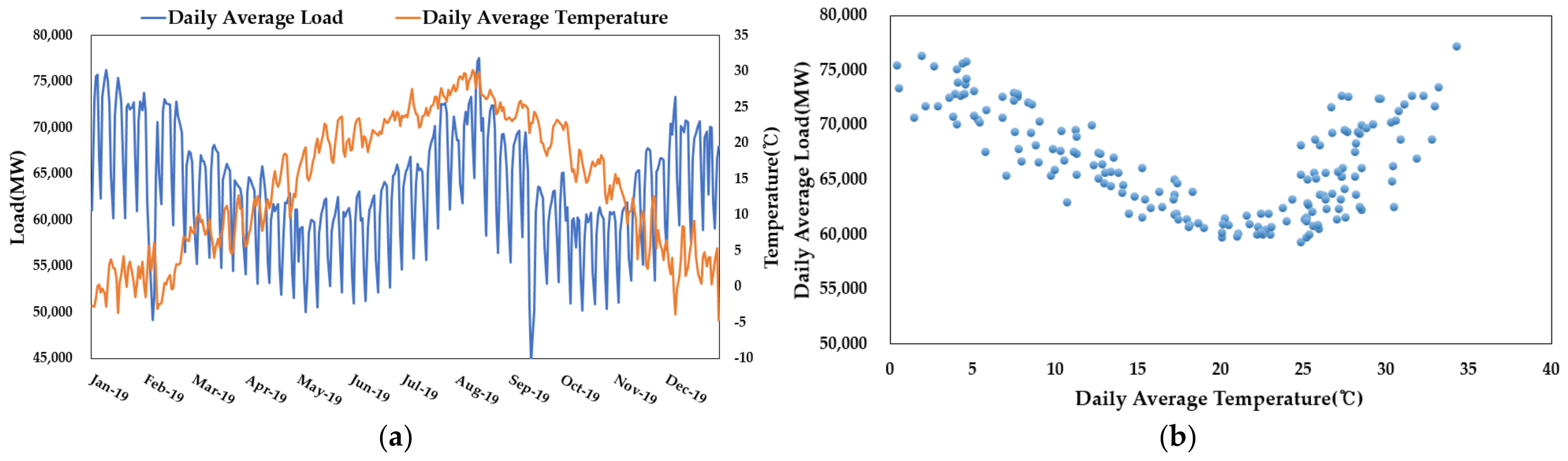
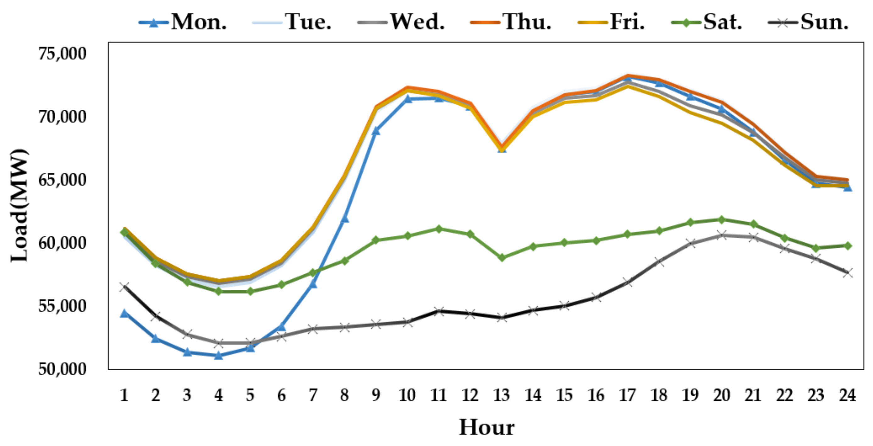
Electric load changes periodically according to calendar factors (such as seasons, day of the week and holidays) and is affected by exogenous factors (such as economic, population and weather). For accurate load forecasting, it is necessary to analyze the relationship between electric load and exogenous variables. In the short term, the electric load is highly related to weather factors and calendar factors. The weather factor that is known to have the greatest impact on electric load is temperature [11,16]. Changes in temperature have a very large impact on heating and cooling energy consumption. In addition, the electric load shows different patterns depending on the characteristics of the day (such as weekdays, weekends and holidays). In South Korea, the proportion of electrical energy consumption in the industrial sector is high [5]. On weekdays, when industrial production is active, electrical energy consumption is higher than on weekends. In the case of Monday, the electric load before noon is lower than that of other weekdays due to the influence of the previous day—Sunday. The electric load characteristics, according to exogenous variables, are shown in Figure 1. Figure 1a shows the daily interval-valued average load and the average temperature in 2019, presenting the periodic change in electric load according to the season. Figure 1b shows a scatter plot of daily average temperature and peak load in 2019, indicating a high positive or negative correlation, or a low correlation, depending on the temperature range. Figure 2 shows the average load pattern by day of the week in 2019, which is largely classified into Monday, Saturday, Sunday and weekdays, except for Monday.
With the spread of renewable energy, the number of small-scale BTM solar PV generators that do not meter the amount of generation in real-time is increasing. Electric load in South Korea refers to the amount of generation metered at the generator output terminal. In the case of a small-scale solar PV generator of equal to or less than 1 MW, there is no imposed obligation to meter the amount of generation in South Korea’s power system [4]. These small-scale solar PV generators are classified as BTM generators and reduce the electric load compared with actual electrical energy consumption. The amount of BTM solar PV generation fluctuates depending on the weather. Accordingly, the volatility of electric load between sunny day and cloudy day is increasing, which causes uncertainty in load forecasting. The volatility of electric load is shown in Figure 3. Figure 3a shows the difference in electric load between a sunny day and a cloudy day in the spring of 2019. During the spring period in South Korea, the effect of temperature on electric load is minimal. At this time, most of the difference in electric load between a sunny day and a cloudy day is caused by the influence of BTM solar PV generator and the load used by lighting appliances. Figure 3b shows the statistics of solar PV capacity and the difference in electric load between a sunny day and a cloudy day by year. With the spread of solar PV generators, the difference in electric load between a sunny day and a cloudy day is also increasing.
As the penetration rate of BTM solar PV generators increases, the correlation between weather factors and electric load is also changing. In the past, the weather factor that had the greatest influence on electric load was temperature. However, the correlation between temperature and electric load is decreasing due to the distortion of the electric load caused by the amount of BTM solar PV generation. On the other hand, for solar radiation and cloud cover—which are highly related to the amount of solar power generation—the correlation with electric load is increasing. The correlation between electric load and weather factors by year is shown in Figure 4.
3. Proposed Methodology
This section describes the process of the proposed algorithm considering the amount of BTM solar PV generation. The overall framework of the proposed algorithm is shown in Figure 5. If historical BTM solar PV generation is estimated, the distortion between electric load and actual electrical energy consumption will be almost eliminated. Then, the influence of exogenous variables on electric load can be well reflected, and thus a more accurate load forecasting can be achieved. Therefore, using historical data, we estimate the capacity of the BTM solar PV generators by considering the effects of temperature and load used by lighting appliances. Using the estimated historical BTM solar PV generation, a reconstituted load is estimated from which the distortion of the electric load is removed. Finally, load forecasting is conducted using the reconstituted load as a target value in the XGBoost model. The details of the procedure are presented in the following subsections.
3.1. Data Preparation
The databases used for load forecasting are electric load, weather and a solar PV generator dataset. Here, the electric load is the historical load of the Korean power system and is the sum of the power generation metered at the generator output terminal. The weather factors are provided by the Korea Meteorological Administration (KMA) [27]. The large-scale solar PV generator dataset includes the amount of power generation and capacity, and it is limited to generators of above 1 MW, for which, power generation is metered in real-time.
3.2. Estimated the Amount of BTM Solar PV Generation
In the case of a small-scale solar PV generator of equal to or less than 1 MW, there is no imposed obligation to meter the amount of generation in real-time in the Korean power system [4]. These small-scale PV generators are classified as BTM generators and cause distortion between electric load and actual electrical energy consumption. For accurate load forecasting, this distortion should be eliminated, and for this purpose, the historical amount of BTM solar PV generation is estimated.
The BTM solar generators are installed in different locations and with different setups (tilt angle, azimuth and panel type). Detailed information about the BTM solar PV generator is difficult to know, and it is also very difficult to estimate the amount of power generation. Therefore, the amount of BTM solar PV generation is estimated using large-scale solar PV data. In this case, it is assumed that the efficiency of the large-scale solar PV generators and the BTM solar PV generators are similar. First, we downscale the capacity of large-scale solar PV generators to unit capacity. Then, the power generation per unit capacity of large-scale solar PV generator is selected as the “standard solar PV generation”. BTM solar PV generation approximation is shown in Equation (1), as follows:
where denotes the BTM solar PV generation (MW) at time denotes large-scale solar PV generation at time , denotes the capacity of large-scale solar PV generators and denotes the estimated capacity of BTM solar PV generator. Here, is unknown. Therefore, it is necessary to estimate the capacity of the BTM solar PV generators to estimate the amount of BTM solar PV generation.
In the short-term, the electric load is mainly dependent on weather and calendar factors, especially the day of the week, holidays, temperature and solar radiation. The calendar factors change the load pattern according to the characteristics of the day. Temperature is a factor that changes heating/cooling energy consumption, and solar radiation is a factor that changes the amount of solar PV generation and load used by lighting appliances. If the influence of weather and calendar factors on electric load is minimized, the deviation of loads is also minimized. Using this assumption, the capacity of the BTM solar PV generators is estimated [26]. The load in spring or autumn, which has a little effect of temperature on load, is selected, and only loads on weekdays except Monday and holidays are used to remove the change in load due to calendar factors.
The base temperature is a fundamental consideration at calculating cooling degree day (CDD) and heating degree day (HDD), and it is one of the metrics that determines the heating and cooling energy consumption [28]. If the daily temperature is within the base temperature range, it means that heating and cooling energy consumption is minimized. When the daily temperature is within the base temperature range, the main cause of the load fluctuation is the change in the amount of solar PV generation. Therefore, the base temperature range with the maximum correlation between the standard solar PV generation and electric load is estimated using grid search. Figure 6 shows a scatter plot of electric load and standard solar PV generation in the autumn of 2019 for days filtered using the base temperature range.
The BTM solar PV generation increases in proportion to solar radiation and the load used by lighting appliances is inversely proportional to solar radiation. To analyze the impact of BTM solar PV generation alone, it is necessary to eliminate the impact of the load used by lighting appliances. When the penetration level of BTM solar PV generators is high, it is difficult to separate the load used by lighting appliances from the electric load. Therefore, load used by lighting appliances is estimated using load data from 2000 to 2005, when the penetration level of solar PV generators is very low. To consider only the impact of the load used by lighting appliances, the days filtered by the estimated base temperature are used. Sunny days and cloudy days are classified according to solar radiation, and the difference between electric load on cloudy days and electric load on sunny days is estimated as the amount of fluctuation in the load used by lighting appliances [26]. As the economy and population grew, the electrical energy consumption increased, and the load used by lighting appliances also increased. To reflect these effects, the standard load is used. Standard load means load calculated by considering only the effect of economic growth excluding other exogenous factors [29]. The fluctuation of the load used by lighting appliances is assumed to be a ratio of the standard load, which is calculated as Equation (2), as follows:
where denotes the fluctuation of the load used by lighting appliances at time , denotes the standard load at time and denotes the ratio of the fluctuation of the load used by lighting appliances to the standard load. The fluctuation of the load used by lighting appliances is calculated based on a sunny day, so this fluctuation on a sunny day is 0.
To minimize the impact of solar radiation on electric load, it is necessary to calibrate the fluctuation caused by the load used by lighting appliances and the BTM solar PV generator. The reconstituted load method considering the load used by lighting appliances is defined using the previously estimated fluctuations of the load used by lighting appliances and the standard solar PV generation. The reconstituted load, considering the load used by lighting appliances, is calculated by Equation (3), as follows:
where denotes the reconstituted load considering the load used by lighting appliances at time , denotes sum of the generation that can be metered by power system operators at time , denotes the BTM solar PV generation at time and denotes the fluctuation of the load used by lighting appliances at time .
Finally, the capacity of the BTM solar PV generators is estimated using the reconstituted load method considering the load used by lighting appliances. The reconstituted load, considering the load used by lighting appliances, has very little correlation with the change in solar radiation. If electric loads of the days filtered by the base temperature are built as a reconstituted load, the variance between reconstituted loads is minimized. Since the capacity of the BTM solar PV generators is unknown, grid search is used to estimate capacity. When the variance between the reconstituted loads achieves the minimum value, the capacity of this point is estimated as the capacity of the BTM solar PV generators.
In seasons except for spring and autumn, there are few days within the base temperature range. Therefore, the estimation capacity of BTM solar PV generators is performed for May in spring and October in autumn. In months except for May and October, the capacity of the BTM solar PV generators is estimated based on regression. The capacity of the BTM solar PV generators estimated based on regression in 2019 is shown in Figure 7.
3.3. Load Forecasting Method Considering BTM Solar PV Generation
In the existing studies, the impact of weather factors and calendar factors on the electric load was mainly reflected in load forecasting [6]. However, the characteristic of electric load changes according to the high penetration rate of BTM solar PV generators. From the analysis in Section 2, it can be seen that the correlation between weather factors and electric load is also changing. Simply using the weather factors as an input feature has a limit in reflecting the distortion of electric load due to the amount of BTM solar PV generation in the load forecasting. Therefore, the reconstituted load method that can remove this distortion is used. The reconstituted load is calculated by Equation (4), as follows:
where denotes the load that is eliminated distortion of electric load at time , denotes sum of the generation that can be metered by power system operators at time and denotes the BTM solar PV generation at time .
The reconstituted load is calculated by adding the amount of BTM solar PV generation to the electric load. The comparison of the correlation between electric load, reconstituted load and temperature in 2019 are shown in Figure 8. The correlation between the reconstituted load and temperature is higher than the correlation between electrical load and temperature.
The input variables used for load forecasting are shown in Table 1. The weather variables are seven factors, including temperature, which has a high correlation with the electric load. The weather variables used as input features in load forecasting are selected through correlation analysis. Load patterns change differently depending on the day of the week and holidays. To distinguish them, day of the week and holiday codes are used as calendar variables [30]. As the target variable, the historical reconstituted load is used to reflect the impact of BTM solar PV generation.
If the reconstituted load is predicted as the target value, the output value is the reconstituted load. For the system operator to use the predicted value, it is necessary to post-process the reconstituted load into the electric load. Reconstituted load post-processing is calculated by Equation (5), as follows:
where denotes the predicted electric load at time , denotes the predicted reconstituted load at time and denotes the predicted BTM solar PV generation at time .
3.4. Modeling of XGBoost
The XGBoost is a decision tree-based algorithm that uses a boosting method and was proposed by Tianqi Chen in 2016 [31]. Boosting is a method to improve prediction accuracy by training a sequence of weak tree models, each compensating for the residuals of the preceding tree model. However, the boosting method has disadvantages in that it is time exhaustive and overfitting. The XGBoost algorithm has evolved the performance of the existing boosting model through tree pruning, parallelization and regularization terms. The XGBoost algorithm just started to be applied to various fields, and there are still a few papers applied to the field of load forecasting [17]. The XGBoost algorithm is proposed for day-ahead load forecasting with various advantages. The XGBoost regressor predicted value is calculated by Equation (6) [32], as follows:
where denotes the predicted value, denotes the th tree model, denotes the input feature, denotes the number of trees and denotes the functional space that contains set of trees. The objective function in the XGBoost regressor includes a regularization term and is defined by Equation (7) [32], as follows:
where denotes the loss function mean squared error (MSE), denotes the actual value and denotes the regularization term that imposes a penalty on model complexity. The regularization term is defined by Equation (8) [32], as follows:
where denotes the number of leaves, denotes the th vector of scores on leaves and and denote the penalty factors.
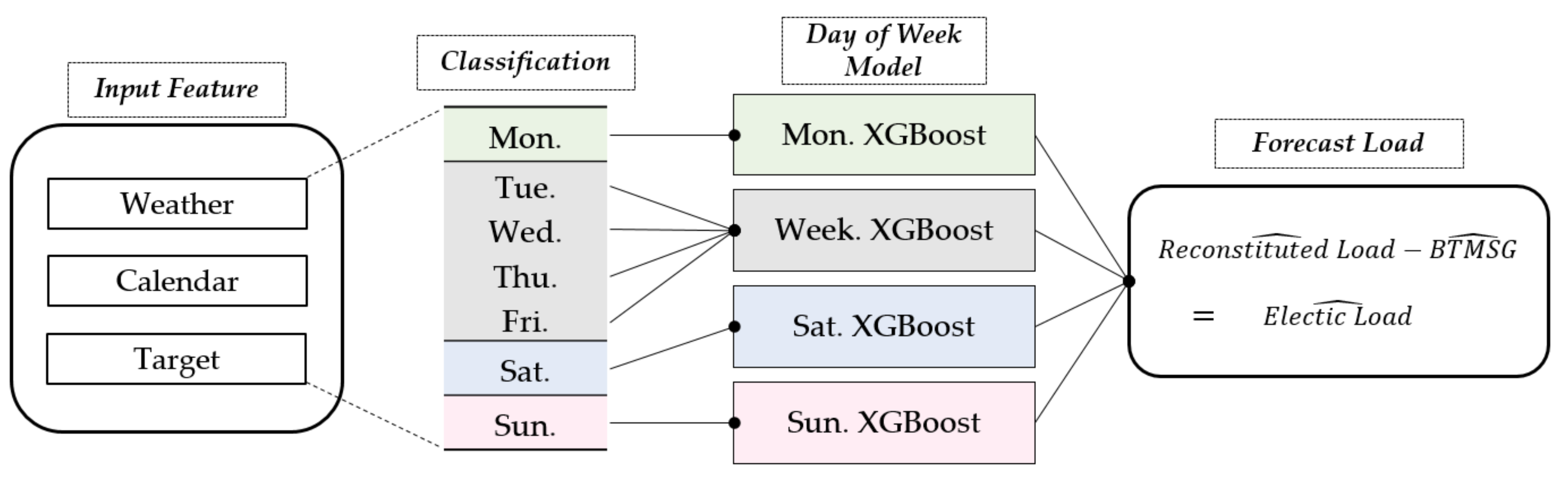
XGBoost is a tree-based model that branches data according to input features and uses the branched data for prediction. If the historical electric load used as the training dataset is different from the day of the week of the target date, it affects the performance and learning time of the model. Therefore, we propose a day-of-week (DoW) model that classifies the training data according to the forecast target date. The load forecasting process of the DoW XGBoost model is shown in Figure 9.
The load is one of the time series data and forecasted using historical data. Therefore, the time series validation method is used for hyperparameter tuning. In the proposed load forecasting algorithm, the training data is updated every timestep (1 day) to continuously reflect the trend of the load. For this, the sliding window-based time series validation is used among cross-validation methods [14]. When load forecasting under real conditions, it is difficult to use the data of the forecasting performed day. Therefore, the gap of one day is placed between validation and training. A grid search is used for hyperparameter tuning, and the parameter with the lowest MSE for the validation dataset is selected. The sliding window-based time series validation method is shown in Figure 10, and the main parameters of the XGBoost algorithm are shown in Table 2 [33].
4. Case Studies
4.1. Input Feature Selection and Hyperparameter Tuning
The majority of the existing load forecasting methods mainly used temperature as a weather factor. With the spread of BTM solar PV generators, the effect of temperature on electric load decreased, and the influence of weather factors, such as solar radiation and humidity, increased. Accordingly, it is necessary to use weather factors that have a high influence on electric load for accurate load forecasting.
The weather prediction factors published by the KMA are temperature, humidity, wind speed and cloud cover [27]. The weather input features used for load forecasting are selected through correlation analysis between load and weather factors. Figure 11 shows the comparison of the correlation between electric load, reconstituted load and weather factors in 2019. In the case of electric load, it can be seen that there is a high correlation with temperature, humidity and cloud cover. On the other hand, in the case of reconstituted load, it was confirmed that the correlation with temperature increased and the correlation with the remaining weather factors decreased.
Case studies are performed using three models to compare predictive performance. The first model is a time series-based simple exponential smoothing (SES) model in which historical load data and temperature data are considered [11]. The second model is an ML-based LSTM-FC model, in which historical load data and temperature data are considered [16]. The third model is the XGBoost-based model, without BTM solar PV generation. The proposed model reflects the impact of BTM solar PV generation by applying the reconstituted load method. Based on the analysis result of the correlation in Figure 11, the third model uses temperature, humidity and cloud cover and the proposed model uses temperature as weather input feature. Table 3 shows the weather input feature and target data for the proposed method and the three forecasting methods for comparison.
The proposed DoW XGBoost model uses different train dataset according to the forecast target date. In addition, since the input features are different depending on the case, it is necessary to optimize the parameters for each forecasting model. Hyper-parameter optimization is an important factor in determining the performance and speed of a model. The proposed model uses gbtree as a default, and hyper-parameter tuning was performed for Max_depth, Min_child_weight and subsample. Other parameters were set as default. Grid search was used for parameter estimation, and the hyper-parameter search result is shown in Table 4.
4.2. Empirical Results and Analysis
To verify the effectiveness of the proposed day-ahead load forecasting algorithm, a case study is performed for day-ahead load forecasting for the Korean power system in South Korea, where the peak load of 2020 was 89,091 MW. Measured values of weather factors are used to avoid performance degradation due to weather forecast errors. The error is evaluated using the mean absolute percentage error (MAPE) and root mean squared error (RMSE). MAPE and RMSE are shown in Equations (9) and (10), respectively, as follows:
where denotes the number of outputs, denotes Actual load and denotes forecasted load.
The day-ahead load forecasting simulation is performed using 630 days excluding holidays in 2019 and 2020 as test data. For example, when load forecasting is performed on 10 January 2020, the hourly electric load on 11 January 2020 is forecasted. In this case, data used as input are data up to 9 January 2020. During the simulation period, load forecasting is performed every day for 630 days excluding holidays, and a total of 630 × 24 h of electric load value is forecasted. In addition, the estimated capacity of BTM solar PV generators increased monotonically from 7900 MW in January 2019 to 13,300 MW in December 2020. To analyze the performance change, according to the penetration rate of BTM solar PV generator, the accuracy is compared by year. In addition, to verify the accuracy improvement through the reflection of the BTM solar PV generation, the error is analyzed by time. Figure 12 and Figure 13 show the MAPE of the forecasting methods by year.
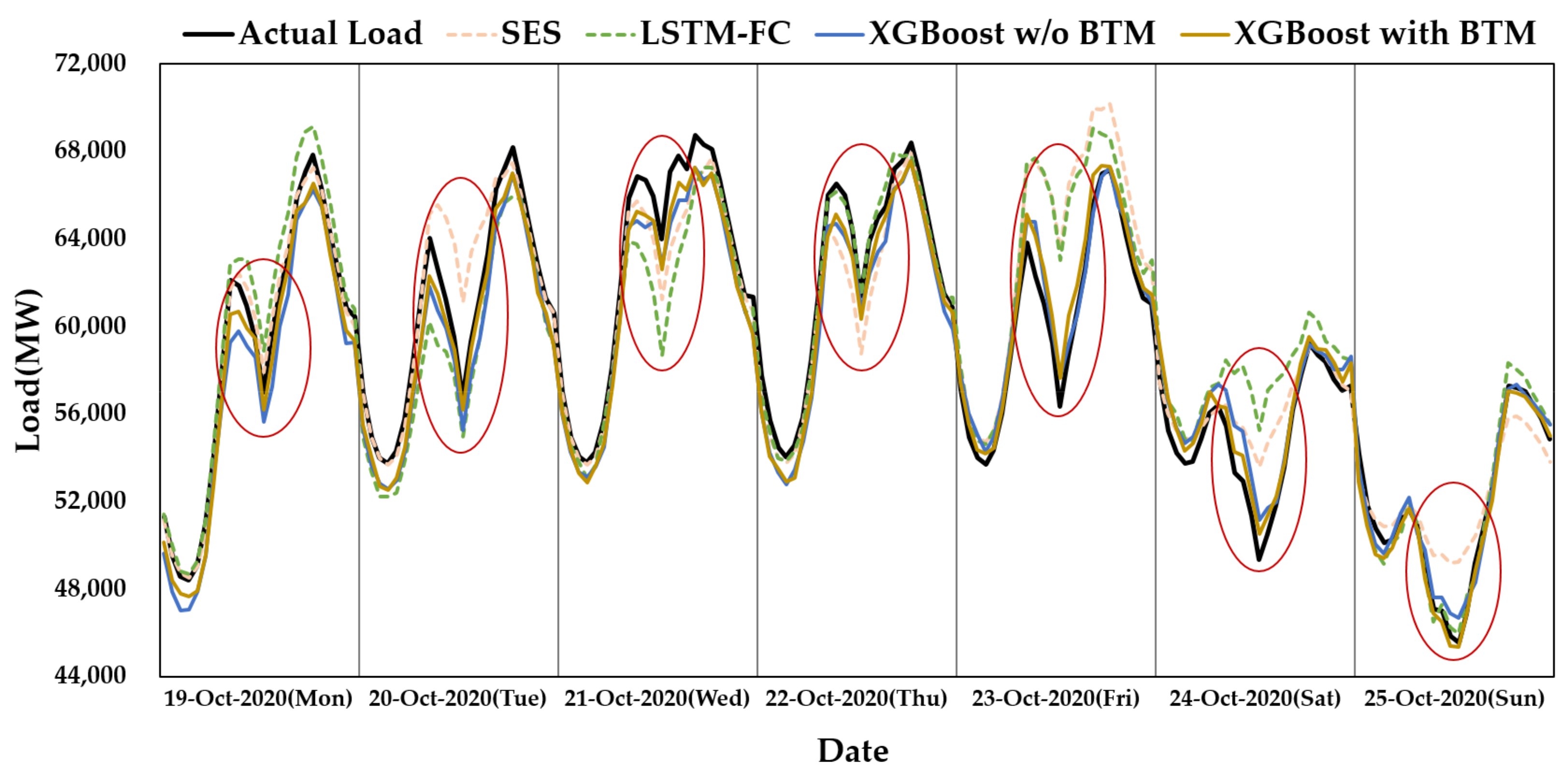
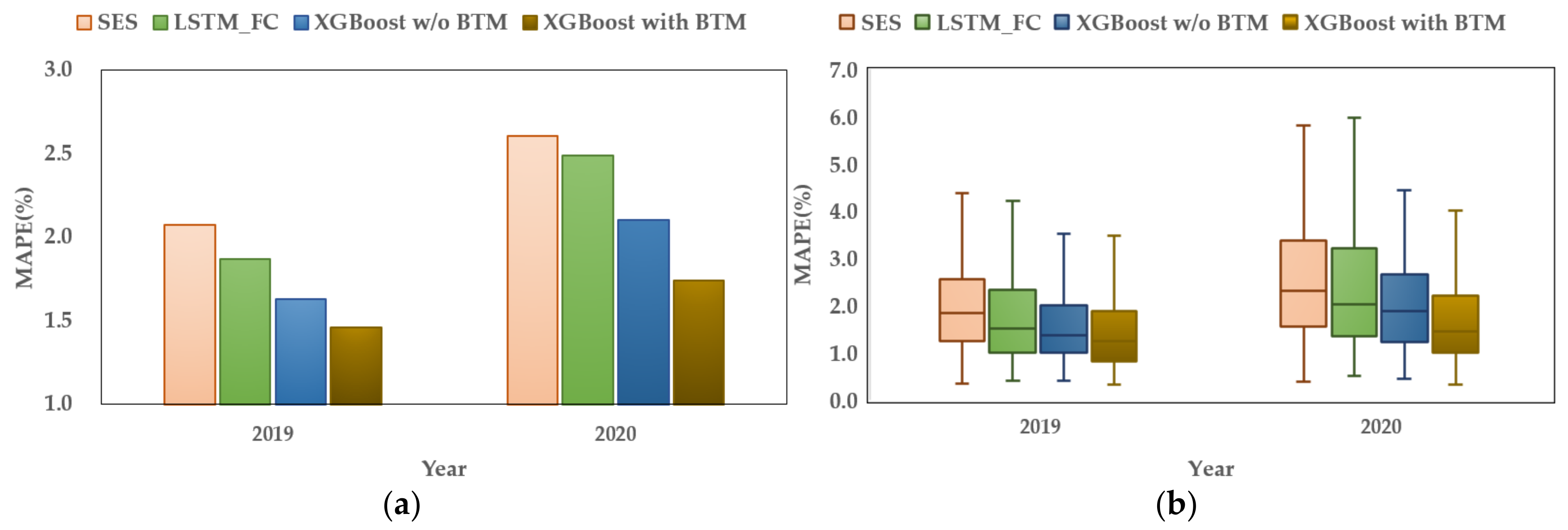
Figure 12a shows the total MAPE for four methods in 2019 and 2020. It was confirmed that the accuracy of the proposed model, XGBoost with BTM, was superior to that of the other three methods. The accuracy of the proposed algorithm was improved by 0.60 percentage points (%p) and 0.85%p in 2019 and 2020, respectively, compared with the MAPE of the SES model. Figure 13 shows the hourly MAPE for four methods in 2019 and 2020. The amount of solar PV generation is small at sunset and sunrise times, and the MAPE of the forecasting methods are similar at sunset and sunrise times. On the other hand, it can be seen that the MAPE of the forecasting methods differs more significantly between 8:00 and 18:00 when solar PV generation is being produced. The improvement of the accuracy of forecasting electric load was the best at 13:00, when the amount of solar PV generation was the highest. The accuracy of the proposed model, XGBoost with BTM, improved by 1.25%p and 2.43%p in 2019 and 2020, respectively, compared with the MAPE of the SES model. An even greater improvement in forecasting error was achieved due to the increase in the penetration rate of BTM solar PV generators in 2020 compared with 2019. To have a closer look at the output and load profiles, the resulting data for one week in October 2020 are shown in Figure 14.
Figure 14 shows the results of the forecasting methods for the week of October 2020. October is autumn, and the electric load is lower than in winter and summer because the heating and cooling energy consumption is small. Accordingly, the impact of the amount of BTM solar PV generation on electric load becomes relatively large. The red ellipses in Figure 14 show the daytime load forecasting results. The proposed method, XGBoost with BTM, can reflect the amount of BTM solar PV generation, so the daytime residual is small, but other forecasting methods confirmed that the residual was large. As the amount of BTM solar PV generation increases, electric load and electrical energy consumption differ, causing distortion of electric load. This distortion of electric load causes the peak and valley loads to shift in time. Peak load refers to the highest electric load during the day, and valley load refers to the lowest electric load during the day. The summary of errors of load forecasting by the forecasting methods during the simulation period is shown in Table 5.
As shown in Table 3, the proposed algorithm, XGBoost with BTM, improved the prediction accuracy compared with other methods. Because the SES model and the LSTM-FM model only consider the temperature for a weather input feature, it is difficult to reflect the impact of the BTM solar PV generation. The forecasting error of the SES model and the LSTM-FC model was relatively large. In the XGBoost model without BTM, the MAPE was reduced by additionally using humidity and cloud cover. The improvement was slight because it was difficult to reflect the increase in the penetration rate for BTM solar PV generators. The proposed algorithm, XGBoost with BTM, can reflect the impact of BTM solar PV generation through the reconstituted load method, showing the best accuracy among the forecasting methods. The distortion of the electric load was solved by estimating the amount of BTM solar PV generation and adding it to the electric load. As a result, the correlation between temperature and electric load was increased to improve the accuracy of load forecasting. It was confirmed that the prediction error during the daytime with a lot of solar PV generation was significantly improved, and the prediction error for the peak load and the valley load was also improved.
5. Conclusions
As solar PV generation expands and the capacity of BTM generators increases, the uncertainty of day-ahead load forecasts increases. In order to overcome this problem, an XGBoost-based, day-ahead load forecasting algorithm, considering behind-the-meter solar PV generation, is proposed. The amount of BTM solar PV generation causes distortion, in which electric load and electrical energy consumption differ. This distortion increases the uncertainty of load forecasting. In the proposed algorithm, the amount of BTM solar PV generation is estimated, and the reconstituted load method that adds BTM solar PV generation to electric load is used. Case studies are performed for the Korean power system in South Korea. As a result of the case studies, the accuracy of the proposed algorithm was improved by 21% and 29% in 2019 and 2020, respectively, compared with the MAPE of the LSTM-FC model that does not reflect the impact of BTM solar PV. Similarly, the RMSE of the proposed algorithm was also improved by 430 MW and 830 MW in 2019 and 2020, respectively. Improving the accuracy of load forecasting can contribute to and improvement of the economic efficiency of power systems’ operation and power market operation.
In the paper, BTM is limited to only solar PV generators. However, various distributed energy sources, such as energy storage systems (ESS) and electric vehicles (EV), are spreading and expanding, and these energy sources will add uncertainty to future electric load forecasts. Future works on load forecasting will attempt to reflect the effects of various energy sources.
Author Contributions
Conceptualization, D.-J.B., B.-S.K. and K.-B.S.; methodology, D.-J.B. and K.-B.S.; software, D.-J.B. and B.-S.K.; validation, D.-J.B., K.-B.S. and B.-S.K.; formal analysis, D.-J.B., B.-S.K. and K.-B.S.; investigation, D.-J.B.; writing—original draft preparation, D.-J.B. and K.-B.S.; writing—review and editing, D.-J.B., K.-B.S. and B.-S.K.; visualization, D.-J.B.; supervision, K.-B.S.; project administration, K.-B.S. All authors have read and agreed to the published version of the manuscript.
Funding
This research received no external funding.
Institutional Review Board Statement
Not applicable.
Informed Consent Statement
Not applicable.
Data Availability Statement
Not applicable.
Conflicts of Interest
The authors declare no conflict of interest.
References
- Song, K.; Ha, S.; Park, J.; Kweon, D.; Kim, K. Hybrid load forecasting method with analysis of temperature sensitivities. IEEE Trans. Power Syst. 2006, 21, 869–876. [Google Scholar] [CrossRef]
- Park, R.; Song, K.; Kwon, B. Short-term load forecasting algorithm using a similar day selection method based on reinforcement learning. Energies 2020, 13, 2640. [Google Scholar] [CrossRef]
- López, J.C.; Rider, M.J.; Wu, Q. Parsimonious Short-Term Load Forecasting for Optimal Operation Planning of Electrical Distribution Systems. IEEE Trans. Power Syst. 2019, 34, 1427–1437. [Google Scholar] [CrossRef] [Green Version]
- Korea Power Exchange (KPX). Available online: https://www.kpx.or.kr (accessed on 20 August 2021).
- Electric Power Statistics Information System (EPSIS). Available online: https://epsis.kpx.or.kr (accessed on 11 December 2021).
- Eliana, V.; Hector, A.; Rodrigo, S. A Systematic Review of Statistical and Machine Learning Methods for Electrical Power Forecasting with Reported MAPE Score. Entropy 2020, 22, 1412. [Google Scholar]
- Fan, S.; Hyndman, R.J. Short-Term Load Forecasting Based on a Semi-Parametric Additive Model. IEEE Trans. Power Syst. 2011, 27, 134–141. [Google Scholar] [CrossRef] [Green Version]
- Clements, A.E.; Hurn, A.S.; Li, Z. Forecasting day-ahead electricity load using a multiple equation time series approach. Eur. J. Oper. Res. 2016, 251, 522–530. [Google Scholar] [CrossRef] [Green Version]
- Taylor, J.W. Short-Term Load Forecasting with Exponentially Weighted Methods. IEEE Trans. Power Syst. 2012, 27, 458–464. [Google Scholar] [CrossRef]
- Juan, M.V.; Ricardo, C.; Germán, A. Forecasting next-day electricity demand and price using nonparametric functional methods. Int. J. Electr. Power Energy Syst. 2012, 39, 48–55. [Google Scholar]
- Song, K.; Ha, S. An algorithm of short-term load forecasting. Trans. Korean Inst. Electr. Eng. 2004, 53, 529–535. [Google Scholar]
- Chia-Nan, K.; Cheng-Ming, L. Short-term load forecasting using SVR (support vector regression)-based radial basis function neural network with dual extended Kalman filter. Energy 2013, 49, 413–422. [Google Scholar]
- Azadeh, A.; Ghaderi, S.F.; Sheikhalishahi, M.; Nokhandan, B.P. Optimization of short load forecasting in electricity market of Iran using artificial neural networks. Optim. Eng. 2014, 15, 485–508. [Google Scholar] [CrossRef]
- Kaur, A.; Nonnenmacher, L.; Coimbra, C.F. Net load forecasting for high renewable energy penetration grids. Energy 2016, 114, 1073–1084. [Google Scholar] [CrossRef]
- Hadri, S.; NaitMalek, Y.; Najib, M.; Bakhouya, M.; Fakhri, Y.; El Aroussi, M. A Comparative Study of Predictive Approaches for Load Forecasting in Smart Buildings. Procedia Comput. Sci. 2019, 160, 173–180. [Google Scholar] [CrossRef]
- Kwon, B.; Park, R.; Song, K. Short-term load forecasting based on deep neural networks using LSTM layer. J. Electr. Eng. Technol. 2020, 15, 1501–1509. [Google Scholar] [CrossRef]
- Madrid, E.A.; Antonio, N. Short-Term Electricity Load Forecasting with Machine Learning. Information 2021, 12, 50. [Google Scholar] [CrossRef]
- Monforte, F.A.; Fordham, C.; Blanco, J.; Barsun, S.; Kankiewicz, A.; Norris, B. Improving Short-Term Load Forecasts by Incorporating Solar PV Generation: Interim Project Report; California Energy Commission: San Diego, CA, USA, 2016. [Google Scholar]
- Wang, F.; Li, K.; Wang, X.; Jiang, L.; Mi, Z.; Catalao, J.P. A distributed PV system capacity estimation approach based on support vector machine with customer net load curve features. Energies 2018, 11, 1750. [Google Scholar] [CrossRef] [Green Version]
- Li, K.; Yan, J.; Hu, L.; Wang, F.; Zhang, N. Two-Stage Decoupled Estimation Approach of Aggregated Baseline Load under High Penetration of Behind-the-Meter PV System. IEEE Trans. Smart Grid 2021, 12, 4876–4885. [Google Scholar] [CrossRef]
- Bu, F.; Dehghanpour, K.; Yuan, Y.; Wang, Z.; Zhang, Y. A data-driven game-theoretic approach for behind-the-meter PV generation disaggregation. IEEE Trans. Power Syst. 2020, 35, 3133–3144. [Google Scholar] [CrossRef] [Green Version]
- Li, K.; Wang, F.; Mi, Z.; Fotuhi-Firuzabad, M.; Duić, M.; Wang, T. Capacity and output power estimation approach of individual behind-the-meter distributed photovoltaic system for demand response baseline estimation. Appl. Energy 2019, 253, 113595. [Google Scholar] [CrossRef]
- Shaker, H.; Zareipour, H.; Wood, D. A data-driven approach for estimating the power generation of invisible solar sites. IEEE Trans. Smart Grid 2016, 7, 2466–2476. [Google Scholar] [CrossRef]
- Shaker, H.; Zareipour, H.; Wood, D. Estimating Power Generation of Invisible Solar Sites Using Publicly Available Data. IEEE Trans. Smart Grid 2016, 7, 2456–2465. [Google Scholar] [CrossRef]
- Wang, Y.; Zhang, N.; Chen, Q.; Kirschen, D.S.; Li, P.; Xia, Q. Data-driven probabilistic net load forecasting with high penetration of behind-the-meter PV. IEEE Trans. Power Syst. 2017, 33, 3255–3264. [Google Scholar] [CrossRef]
- Bae, D.; Kwon, B.; Woo, S.; Moon, C.; Song, K. The Estimation Algorithm of Behind-the-Meter Solar PV Capacities Considering Lighting Load. Trans. Korean Inst. Electr. Eng. 2021, 70, 742–749. [Google Scholar] [CrossRef]
- Korea Meteorological Agency (KMA) Weather Data Service. Available online: https://data.kma.go.kr (accessed on 20 August 2021).
- Lee, K.; Baek, H.; Cho, C. The Estimation of Base Temperature for Heating and Cooling Degree-Days for South Korea. J. Appl. Meteorol. Climatol. 2014, 53, 300–309. [Google Scholar] [CrossRef]
- Jo, S.; Park, R.; Kim, K.; Kwon, K.; Song, K. Sensitivity Analysis of Temperature on Special Day Electricity Demand in Jeju Island. Trans. Korean Inst. Electr. Eng. 2018, 67, 1019–1023. [Google Scholar]
- Korean Calendar. Available online: https://en.wikipedia.org/wiki/Korean_calendar (accessed on 20 August 2021).
- Chen, T.; Guestrin, C. XGBoost: A Scalable Tree Boosting System. In Proceedings of the 22nd ACM SIGKDD International Conference on Knowledge Discovery Data Mining, San Francisco, CA, USA, 13–17 August 2016; pp. 785–794. [Google Scholar]
- XGBoost Documentation. Available online: https://xgboost.readthedocs.io (accessed on 20 August 2021).
- Scikit-Learn. Available online: https://scikit-learn.org (accessed on 20 August 2021).
Figure 1.
The electric load characteristics according to temperature: (a) the daily interval-valued electric load and temperature in 2019; (b) the scatter plot of daily temperature and electric load in 2019.
Figure 1.
The electric load characteristics according to temperature: (a) the daily interval-valued electric load and temperature in 2019; (b) the scatter plot of daily temperature and electric load in 2019.

Figure 2.
The average electric load pattern by day of the week in 2019.

Figure 3.
The volatility of electric load: (a) difference in electric load between a sunny day and a cloudy day in spring; (b) the capacity statistics of solar PV generator and the difference in electric load between a sunny day and a cloudy day by year.
Figure 3.
The volatility of electric load: (a) difference in electric load between a sunny day and a cloudy day in spring; (b) the capacity statistics of solar PV generator and the difference in electric load between a sunny day and a cloudy day by year.
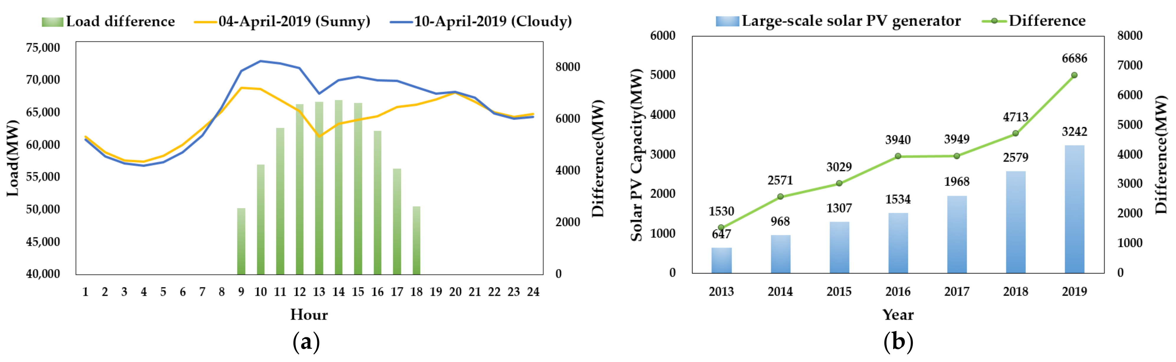
Figure 4.
The correlation between electric load and weather factors by year.
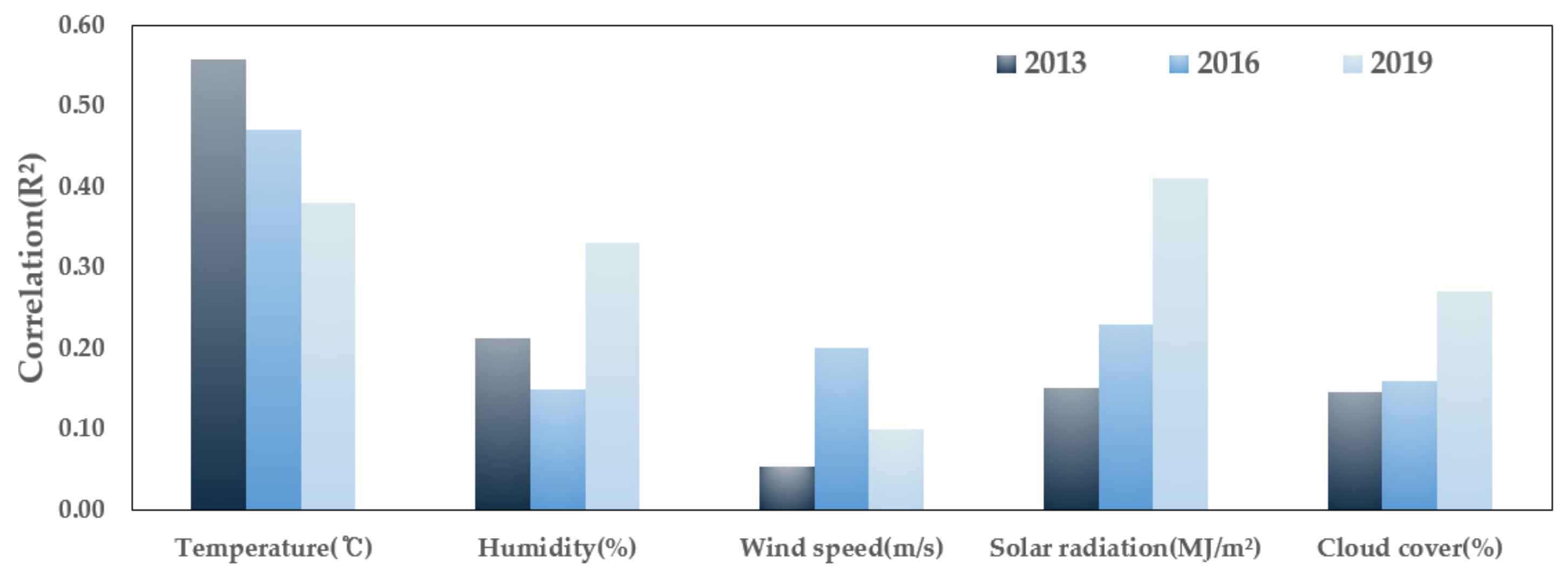
Figure 5.
The overall framework of the proposed algorithm.
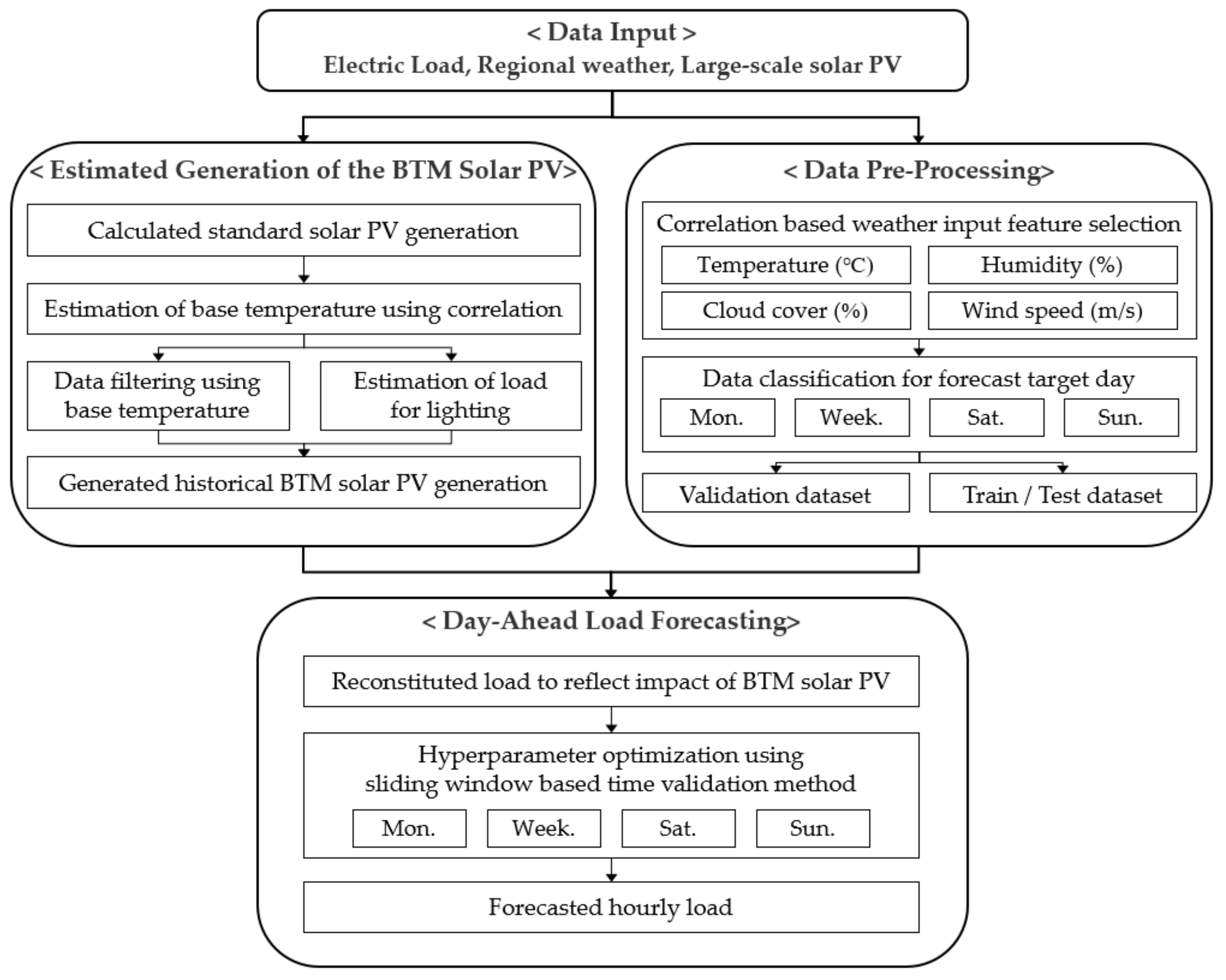
Figure 6.
Scatter plot of electric load and standard solar PV generation in the autumn of 2019: (a) days filtered by the KMA base temperature range (18–26 °C); (b) days filtered by the estimated base temperature range (12–19 °C).
Figure 6.
Scatter plot of electric load and standard solar PV generation in the autumn of 2019: (a) days filtered by the KMA base temperature range (18–26 °C); (b) days filtered by the estimated base temperature range (12–19 °C).
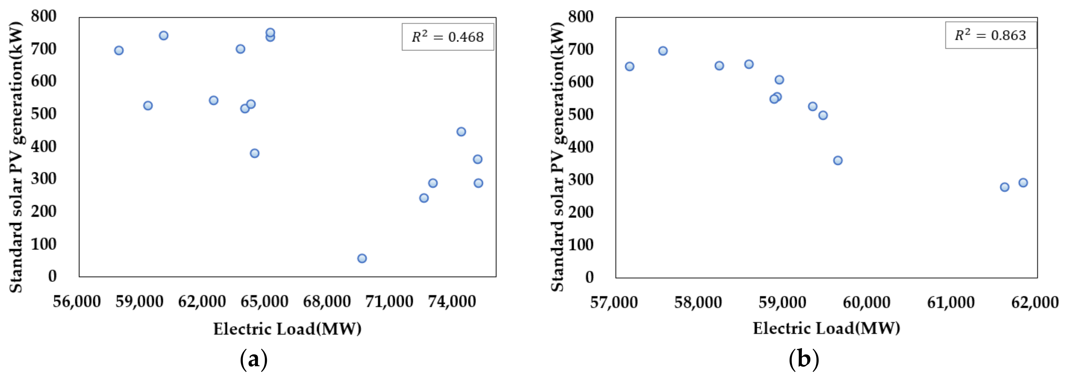
Figure 7.
The capacity of the BTM solar PV generators estimated based on regression in 2019.
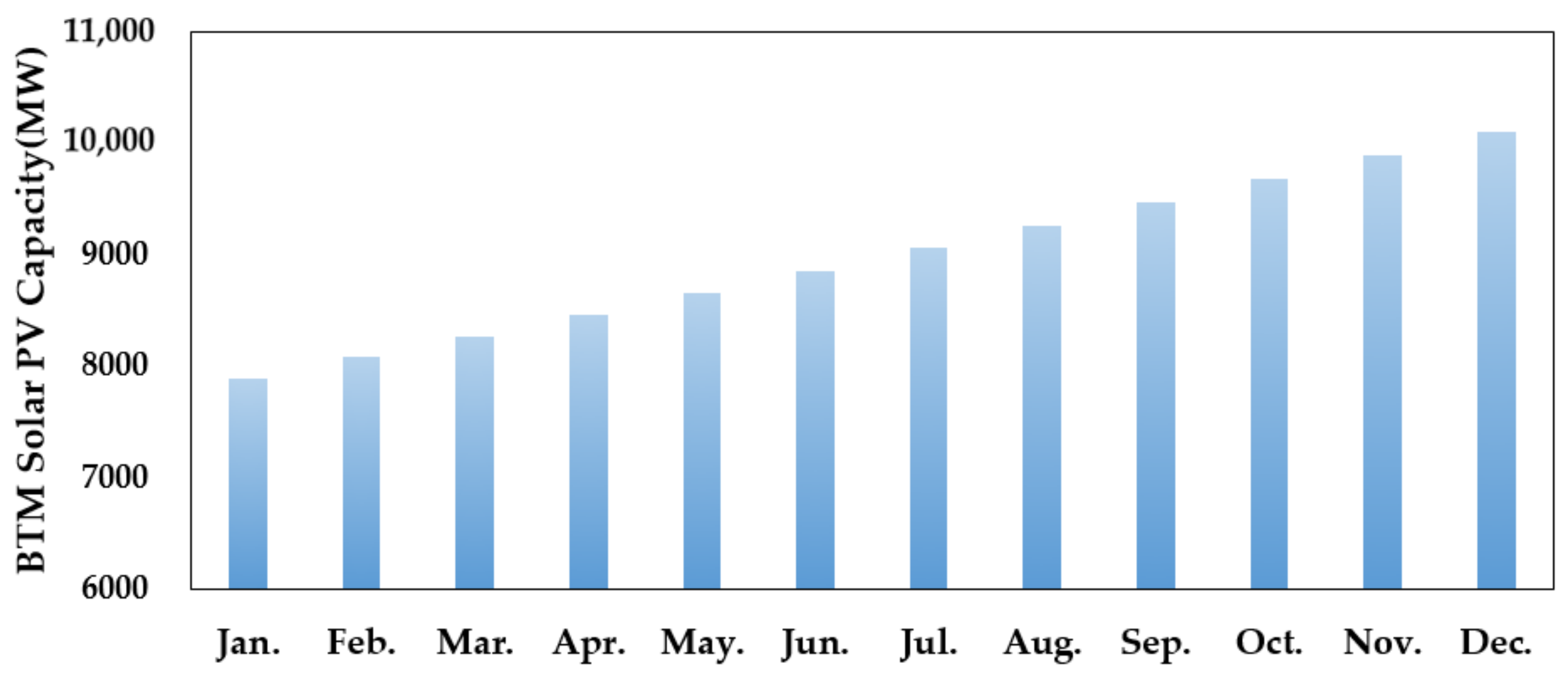
Figure 8.
The comparison of the correlation between electric load, reconstituted load and temperature in 2019.
Figure 8.
The comparison of the correlation between electric load, reconstituted load and temperature in 2019.

Figure 9.
Load forecasting process of the DoW XGBoost model.

Figure 10.
The sliding window-based time series validation method.
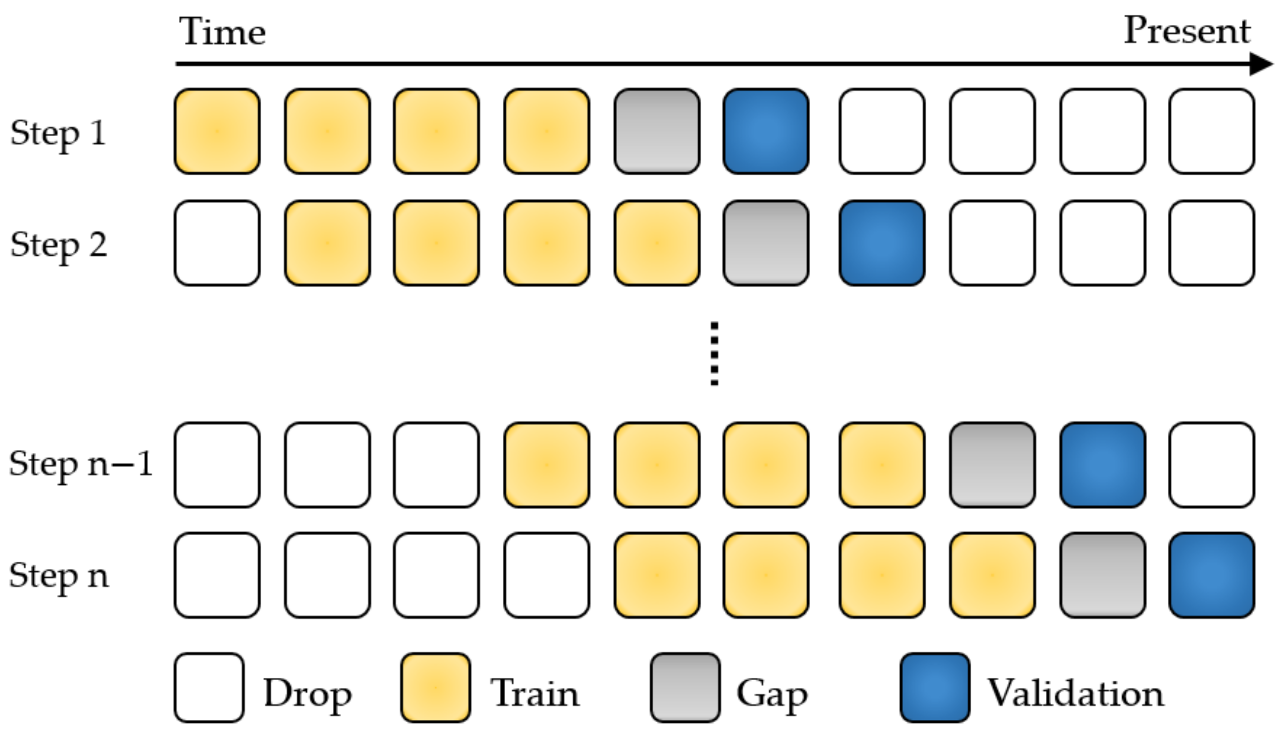
Figure 11.
The correlation between electric load, reconstituted load and weather factors in 2019.
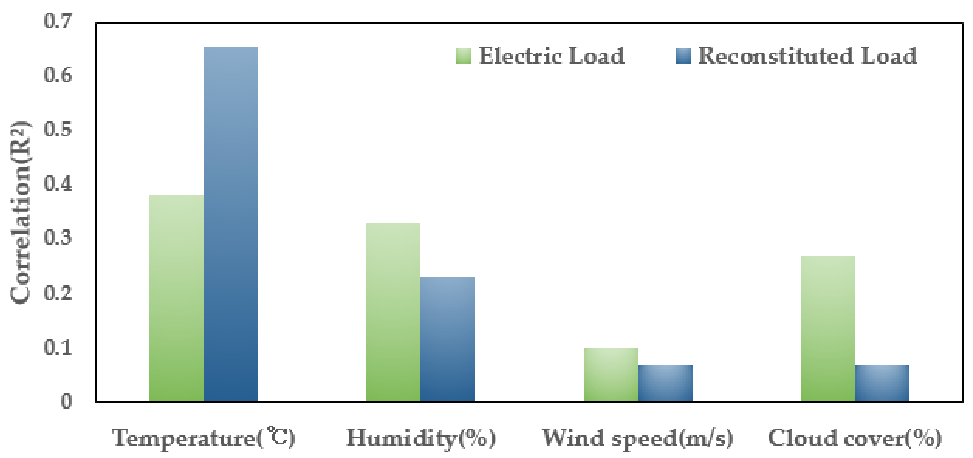
Figure 12.
The MAPE of the forecasting methods by year: (a) bar plot of the average MAPE; (b) box plot of the MAPE.
Figure 12.
The MAPE of the forecasting methods by year: (a) bar plot of the average MAPE; (b) box plot of the MAPE.

Figure 13.
The hourly MAPE of the forecasting methods by year: (a) 2019; (b) 2020.
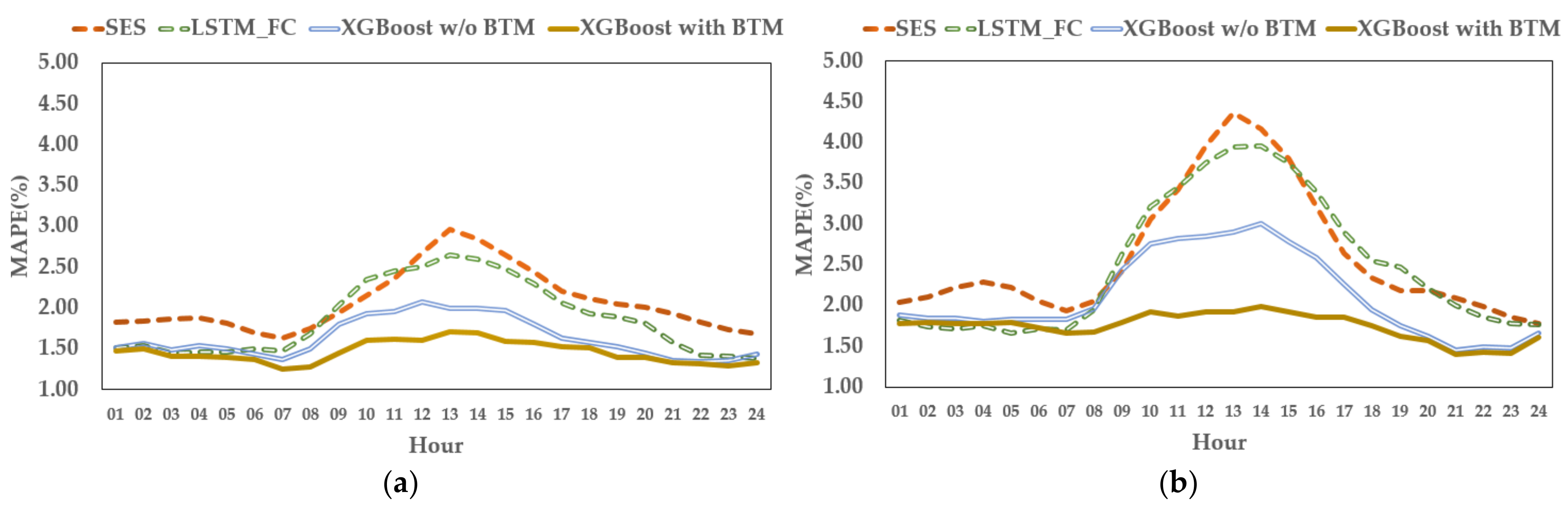
Figure 14.
The day-ahead load forecasting results from 19 October 2020 to 25 October 2020.

Table 1.
The input variables used for load forecasting.
| Variable | Input Feature Name | Value/Unit |
|---|---|---|
| Weather | Hourly Temperature | ℃ |
| Hourly Cloud Cover | % | |
| Hourly Humidity | % | |
| Hourly Wind Speed | m/s | |
| Calendar | Day of the Week Code | 1–7: Mon.–Sun. |
| Holiday Code | 0: Non, 10: Holiday | |
| Target | Reconstituted Load | MW |
Table 2.
The main parameters of the XGBoost algorithm.
| Hyperparameter | Definition | Default |
|---|---|---|
| Booster | Which booster to use | gbtree |
| Max_depth | Maximum tree depth for base learners | 6 |
| Min_child_weight | Minimum sum of instance weight needed in a child | 1 |
| subsample | Subsample ratio of the training instances | 1 |
| n_estimators | Number of gradient-boosted trees | 100 |
Table 3.
The weather input feature and target data for the forecasting methods for comparison.
| Forecasting Method | Weather Input Feature | Target |
|---|---|---|
| SES | Temperature (°C) | Electric Load |
| LSTM-FC | Temperature (°C) | Electric Load |
| XGBoost w/o BTM | Temperature (°C), Humidity (%), Cloud Cover (%) | Electric Load |
| XGBoost with BTM (Proposed Method) | Temperature (°C) | Reconstituted Load |
Table 4.
Hyper-parameter search result.
| Forecasting Method | DoW | Max_Depth | Min_Child_Weight | Subsample |
|---|---|---|---|---|
| XGBoost w/o BTM | Mon. | 6 | 2 | 0.6 |
| Week. | 3 | 2 | 0.9 | |
| Sat. | 3 | 2 | 0.7 | |
| Sun. | 5 | 4 | 0.9 | |
| XGBoost with BTM (Proposed Method) | Mon. | 3 | 4 | 0.9 |
| Week. | 4 | 3 | 0.9 | |
| Sat. | 3 | 2 | 0.8 | |
| Sun. | 4 | 4 | 0.9 |
Table 5.
Performance comparison of forecasting methods for 2019 and 2020.
| Errors | SES | LSTM-FC | XGBoost w/o BTM | XGBoost with BTM | |
|---|---|---|---|---|---|
| 2019 | Total MAPE | 2.06% | 1.86% | 1.63% | 1.46% |
| Peak Load MAPE | 1.91% | 1.83% | 1.58% | 1.57% | |
| Valley Load MAPE | 2.01% | 1.64% | 1.60% | 1.40% | |
| RMSE | 1732 MW | 1693 MW | 1393 MW | 1263 MW | |
| 2020 | Total MAPE | 2.60% | 2.48% | 2.11% | 1.75% |
| Peak Load MAPE | 2.32% | 2.46% | 1.99% | 1.67% | |
| Valley Load MAPE | 2.68% | 2.18% | 2.15% | 1.83% | |
| RMSE | 2124 MW | 2198 MW | 1658 MW | 1368 MW |
Publisher’s Note: MDPI stays neutral with regard to jurisdictional claims in published maps and institutional affiliations. |
© 2021 by the authors. Licensee MDPI, Basel, Switzerland. This article is an open access article distributed under the terms and conditions of the Creative Commons Attribution (CC BY) license (https://creativecommons.org/licenses/by/4.0/).
Share and Cite
MDPI and ACS Style
Bae, D.-J.; Kwon, B.-S.; Song, K.-B. XGBoost-Based Day-Ahead Load Forecasting Algorithm Considering Behind-the-Meter Solar PV Generation. Energies 2022, 15, 128. https://doi.org/10.3390/en15010128
AMA Style
Bae D-J, Kwon B-S, Song K-B. XGBoost-Based Day-Ahead Load Forecasting Algorithm Considering Behind-the-Meter Solar PV Generation. Energies. 2022; 15(1):128. https://doi.org/10.3390/en15010128
Chicago/Turabian StyleBae, Dong-Jin, Bo-Sung Kwon, and Kyung-Bin Song. 2022. "XGBoost-Based Day-Ahead Load Forecasting Algorithm Considering Behind-the-Meter Solar PV Generation" Energies 15, no. 1: 128. https://doi.org/10.3390/en15010128
Note that from the first issue of 2016, this journal uses article numbers instead of page numbers. See further details here.