Abstract
Load forecasting (LF) is essential in enabling modern power systems’ safety and economical transportation and energy management systems. The dynamic balance between power generation and load in the optimization of power systems is receiving increasing attention. The intellectual development of information in the power industry and the data acquisition system of the smart grid provides a vast data source for pessimistic load forecasting, and it is of great significance in mining the information behind power data. An accurate short-term load forecasting can guarantee a system’s safe and reliable operation, improve the utilization rate of power generation, and avoid the waste of power resources. In this paper, the load forecasting model by applying a fusion of Improved Sparrow Search Algorithm and Long Short-Term Memory Neural Network (ILSTM-NN), and then establish short-term load forecasting using this novel model. Sparrow Search Algorithm is a novel swarm intelligence optimization algorithm that simulates sparrow foraging predatory behavior. It is used to optimize the parameters (such as weight, bias, etc.) of the ILSTM-NN. The results of the actual examples are used to prove the accuracy of load forecasting. It can improve (decrease) the MAPE by about 20% to 50% and RMSE by about 44.1% to 52.1%. Its ability to improve load forecasting error values is tremendous, so it is very suitable for promoting a domestic power system.
1. Introduction
Power systems are vital to people’s lives, business activities, industrial development, and scientific research, and can contribute significantly to the development of socio-economic science. The fundamental energy source of an electric power system is primary energy, which, by converting it into electricity, supplies the electricity that people need to carry out their lives, consisting mainly of power generation, transmission, substation, distribution, and electricity use. Therefore, to ensure that users have a safe and reliable power supply, power systems are a solid backing for society and people to achieve efficient energy use. The power load is objective; when it is too light or too heavy, it is not conducive to the power system’s safety, stability, and economic development, so the power system load forecast has many necessities and significance. With the continuous improvement of Taiwan’s installed power generation capacity, the trend of power load changes is becoming more complex, bringing significant challenges to the planning and operation of the power system. Considering the need for a power system to plan future power consumption and master the power consumption situation, it is of great reference value to optimize the power supply process from timeliness, accuracy, and reliability. For short-term load forecasting, the improvement of accuracy and forecasting speed is not only beneficial to the reliable power supply and stable operation of the power system, but also to the control of the power quality, and thus to the power supply system on the social and economic levels. Therefore, it is of great research value to study the improvement of the forecasting model of short-term load forecasting and thus improve the reliability of its forecasting results. Short-term load forecasting is an important research area for the operation and optimization of the power system. However, there are factors of randomness and uncertainty of power load. Thus, accurate forecasting is not easy.
Countless domestic and foreign scholars in this field have carried out substantial research on the earliest artificial forecasting methods and traditional statistical forecasting methods, up to today’s machine learning forecasting methods and combination model forecasting methods. Researchers put forward many effective algorithmic schemes to obtain appropriate research results in their respective eras. These methods include the following: (1) Traditional statistical forecasting methods. The traditional statistical forecasting method is mainly composed of the Regression Analysis method [1,2,3], the Time Series method [4], the Kalman Filter method [5], the Least Square Method [6], neural networks (NNs) [7,8], etc. The basic idea is to build a mathematical model—the optimal combination of multiple influencers of the load or historical data from the last moments of the load. The advantage is that the model has a fast and straightforward forecasting speed, but it is poor for nonlinear data forecasting performance. Once the historical data are missing or have a significant error, it is impossible to construct an ideal mathematical model, affecting forecasting accuracy. With the continuous progress of the power system, the data of power load are growing larger, and the characteristics of factors affecting the change of load are increasing and becoming more complicated. The limitations of the traditional statistical forecasting method are further highlighted, and the scope of application is narrowed step by step. (2) Machine learning forecasting methods. The basic idea of machine learning forecasting and computer technology is based on probability theory, statistics, approximation theory, convex analysis, algorithmic complexity theory, and other disciplines. The calculator’s mighty computing power can mine potential information from large amounts of data, learn from experience, improve itself, and automatically build generalized models for forecasting. The learning strategy can also be subdivided into machine learning that directly uses mathematical methods, including Support Vector Machine (SVM) [9,10], Random Forest (RF) [11], etc. Typical representatives and intelligent algorithms that simulate the learning process of neurons in the human brain include BP Neural Network (BPNN) [12], Machine Learning (ML) [13,14,15], Deep Neural Network (DNN) [16,17], Convolutional Neural Network (CNN) [18,19,20,21], Recurrent Neural Network (RNN) [22,23,24], and Long Short-Term Memory Neural Network (LSTM) [25,26,27,28,29]. Support vector regression (SVR) [30,31,32,33] has the advantages of structural stability, generalization ability, optimal global solution, etc., but its ability to handle significant sample data performance is poor and not sensitive enough to timing data. (3) The combined model forecasting method. Although machine learning forecasting can make up for many problems of traditional statistical forecasting methods, each model has an inherent defect. Selecting historical load characteristics and establishing models can break the continuity and intrinsic laws of the load. With the development of deep learning, the circular neural network model, represented by the Gated Recurrent Unit Network (GRU) [34,35,36], can dig up the potential information in the timing data on its own and describe the change law of the timing data comprehensively.
However, there is also significant sample demand, susceptibility to overfitting, poor generalization ability, etc. Based on the uncertainty and multi-scheme of complex forecasting, the combined model combines multiple single models to obtain more accurate forecasting results and a more robust forecasting model. Such combination models are commonly able to obtain more significant and superior generalization and forecasting performance than a single model. Dash et al., for example, propose a combination model that combines neural networks with Fuzzy Expert Systems (FES) for short-term load forecasting. After the historical load data and weather data are blurred by the membership function, as the neural network input, the network output is also blurred by the membership function, and then the FES is entered. An adaptive fuzzy correction scheme obtains the final load forecasting.
Another example is Che et al., who proposed a support vector regression model based on different “kernels”, using different kernel functions to establish a single-kernel support vector regression model and then combined them according to the inverse ratio of errors. Jihoon et al. sought to overcome the single layer of a deep neural network optimal, super parametric, hidden number, which made it complicated to determine the problem based on the training set. They constructed four different four-layer deep neural network forecasting models, validated and selected super-optimal parameters, and finally, using the primary component regression method based on sliding windows, built a constructive load forecasting model.
In contrast, in this paper, more effective solutions are proposed for some of the shortcomings of these new methods. We propose to establish an electric load forecasting model by applying fusion of the Improved Sparrow Search Algorithm (ISSA) [37,38,39] and Long Short-Term Memory Neural Network (ILSTM-NN). The ISSA is proposed to optimize the parameters of the LSTM-NN as a new method of short-term load forecasting. Then, the nonlinear approximation capability of the ILSTM-NN method itself is used to improve the accuracy of the solution load forecasting. At the same time, we can obtain more accurate load forecasting when dealing with the load under the influence of various factors (such as temperature, humidity, rainfall, holidays, etc.) and consider the individual factors.
2. How Power Load Forecasting Works
Load forecasting is based on meteorological conditions, date patterns, social impact, and system operation status, and a mathematical model for dealing with the past and future loads of electric power is established to determine the power load data at a particular time in the future under the condition of meeting the requirements of specific forecasting accuracy. Set the influence factor of the power load , where p represents the number of influence factors and y represents the power load observation value, using a particular model method to describe the nonlinear relationship between the power load of the influence factor, as in Equation (1):
3. Short-Term Load Forecasting Is Described Using the ILSTM-NN
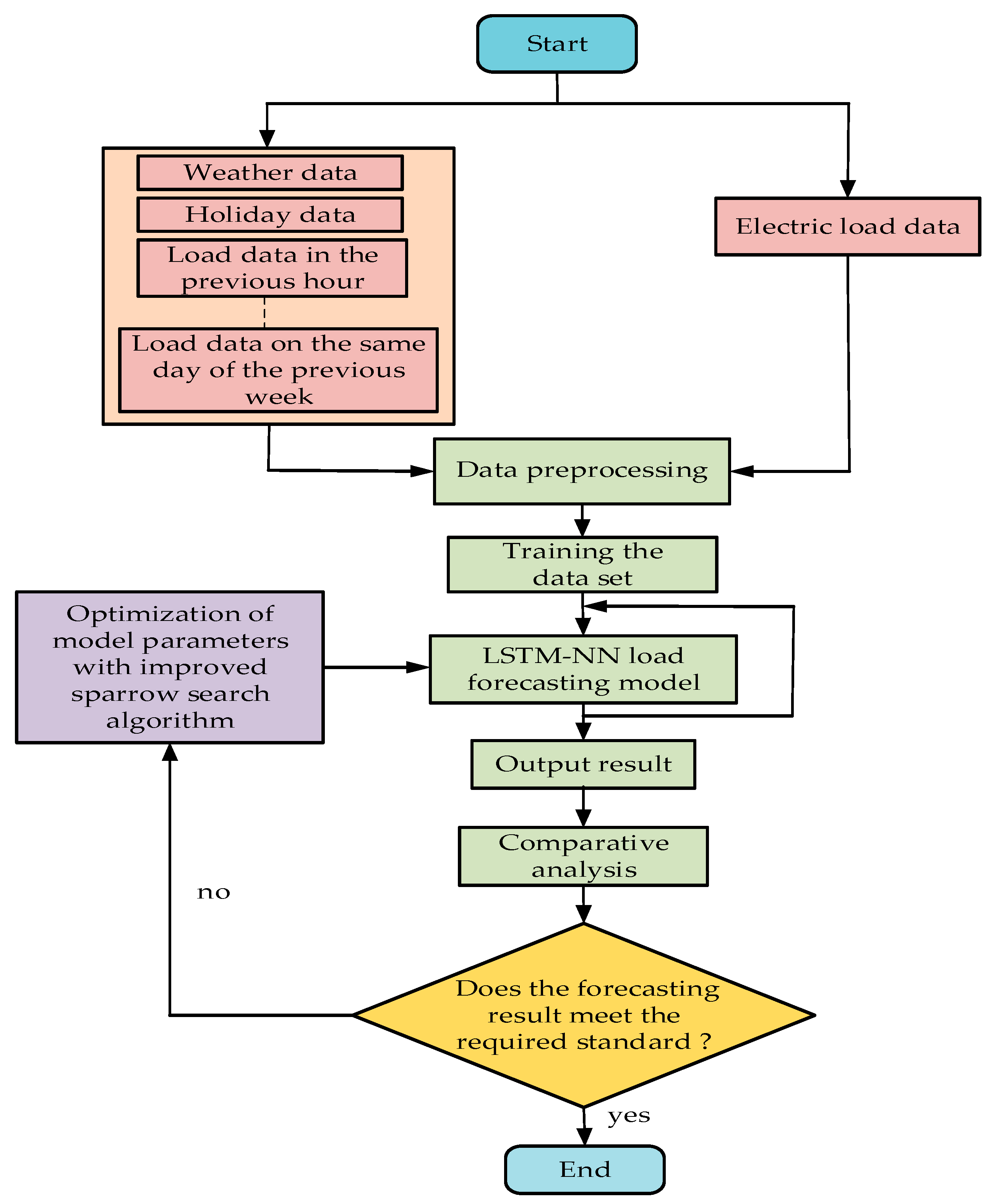
Because the power load is a complete result influenced by many factors, showing a high nonlinear variation law and a limited sample for forecasting, it is difficult for traditional linear methods to forecast accurately based on extensive sample data. Therefore, the ILSTM-NN method is proposed here because it has infinite nonlinear approximation capability and is suitable for power load forecasting. Using an ILSTM-NN to forecast power system load, the first step is to determine the model input, the historical power load, as the essential input, because it is the most crucial factor of the model’s forecasting accuracy improvement. We need to consider the conditions that may affect the change in the load. The correlation between the power load data and the influence factor data is analyzed so that the correlation is extensively filtered out, which helps to improve the model’s forecasting accuracy, and the influence factor data are used as the input of the model. If the input data are not carefully processed and entered directly into the model, the training effect of the model will be poor, so the data input model needs to preprocess the data, mainly to supplement the lack of data, in addition to reducing the data scale of the input data. The preprocessed data can be entered into the model for training, and the trained model outputs forecast data to observe the forecasting effect of the model by comparing the forecasting data with the actual data. Suppose forecasting results do not meet the requirements. In that case, it is necessary to adjust the model parameters to retrain the model and have the forecasting results be compared again until they meet the requirements. The flow chart of ILSTM-NN for power system load forecasting is shown in Figure 1.

Figure 1.
The flow chart of ILSTM-NN for load forecasting.
4. Recurrent Neural Network (RNN)
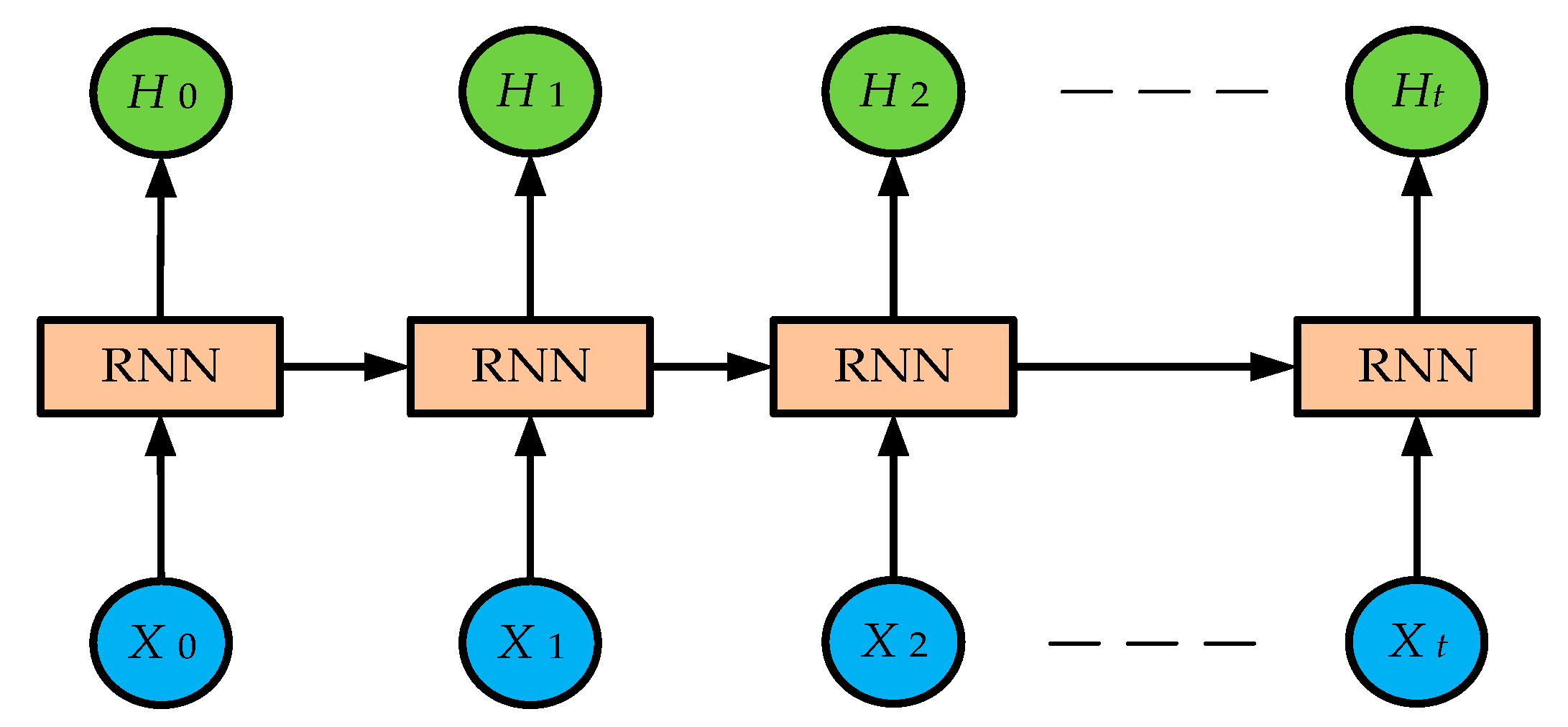
Load forecasting essentially finds a mapping relationship in historical data and reuses it to forecast future power load data. The neural network model has strong memory neural networkability, robustness, and nonlinear learning ability, which can solve power system load forecasting well. LSTM-NN is an improved circulatory neural network algorithm and RNN works in a loop; that is, the output of the last neuron, together with other variables at the next point in time, is re-delivered to the current neuron as an input to the neuron, the data in the loop from the current state to the next state, so the RNN can be expanded to a chained neural network. Figure 2 shows the expanded schematic of the RNN.
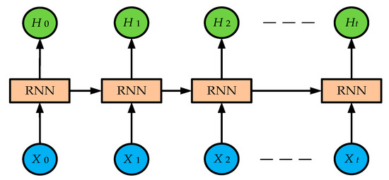
Figure 2.
Expanded schematic of the RNN.
In Figure 2, the input for the neural network unit is Xt, and the output is Ht. RNN is effective at learning and forecasting historical information when the training data are used at short intervals. RNN can still learn historical information and make accurate forecasts. As the time interval of training data increases, the learning ability will weaken. The model will increase with the interval, forget the law of the previous data, the long-term dependence of poor learning ability, and thus, the phenomenon of gradient decline. Power load forecasting needs to learn the long-term load data, find the mapping relationship, and perform forecasting, and the RNN deals with the load forecasting problem; overall, it is challenging to achieve the desired effect.
5. Long Short-Term Memory Neural Network
When an RNN is dealing with a problem with long-term dependency, network-generated gradients disappear, and gradient explosion occurs because back-propagation causes bias to very small or very large values when updating parameters. The birth of LSTM is to better deal with such problems. An LSTM network over the course of training can spontaneously remember the long-term information of data and its relevance in various tasks to achieve suitable predictive results, so it is widely used in machine translation, time series forecasting, and other fields. It is also more helpful than other statistical methods. However, the LSTM-NN model is more complex than the neuron structure of the RNN model, and information is transmitted one by one in the cells of the network (as shown in Figure 3).
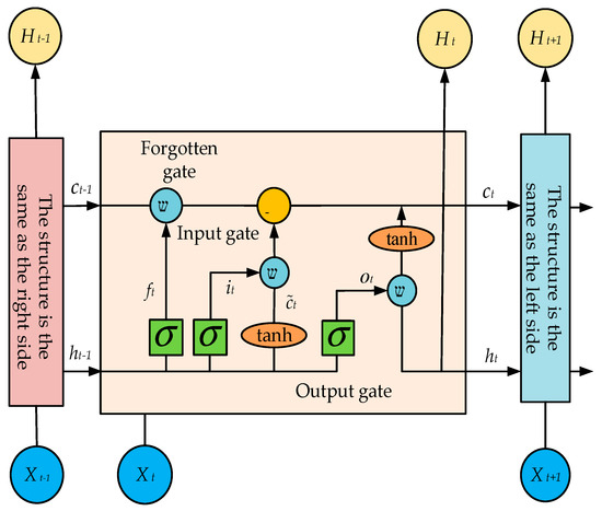
Figure 3.
A diagram of the structure of the LSTM-NN model.
To avoid gradient decline, as in RNN, LSTM-NN uses the “gate” structure to enhance information transmission and communication between cells, including the input gate, the output gate, and the forgetting gate, which learns and forecasts the load data of the power system by controlling the input, output, and historical dependence of neurons. The LSTM-NN operation is as follows:
Equation (2) controls the “forgotten” information of the current neuron from the previous neuron, implemented by the Sigmoid layer known as the “forgotten gate”, , which is an activate function known as a Sigmoid function. are the weights and thresholds of the forgotten gate, respectively. The forgotten gate works by reading the last neuron’s output, , and the current neuron’s input, , entering a value between 0–1 and multiplying with the previous cell state . If the output is 1 multiplied by , representing the previous cell state information, this is a “memory neural network”. If the output is 0 and multiplied by to represent the previous cell state information, this is completely “forgetting”. In this way, the long-term memory of the network model is guaranteed. Equations (3) and (4) together control the input of cells. Equation (3) is implemented by the Sigmoid layer called the “input gate”. After the input gate reads the output of the previous neuron and the current neuron input , it outputs a quantity of 0–1, . In Equation (4), a new candidate vector created by a layer tanh can obtain the current cell state of Equation (5) through , , . are the weight matrix of the input gate and the candidate value, respectively; are the corresponding bias values.
After calculating the information retention of the previous neuron and the input information of the current neuron, the final output is controlled by the Sigmoid layer called the “output gate”. Multiply the current cell state treated by the tanh layer with the Sigmoid (as shown in Equation (6)) obtained by the output gate, and the final output of the current neuron in the resulting Equation (7). are the output gate’s weight and bias values, respectively.
6. Optimization of Load Forecasting Model with Improved Sparrow Search Algorithm (ISSA, Also Named Chaos Sparrow Search Algorithm, CSSA)
6.1. Optimization of LSTM-NN Parameters
The key to studying load forecasting of power systems using LSTM-NN lies in training models. Furthermore, the ultimate purpose of model training is to find a set of optimal parameters (that is, the number of hiding neurons, weight values, bias values, and the number of iterations) so that the forecasting result can be the most accurate. However, the diversity, uncertainty, and correlation of model parameters make determining model parameters extremely complicated. The optimization problem is to find a set of parameter solutions to the problem under certain constraint conditions and have this set of solutions meet the optimality of the problem measurement so that the performance index of the whole system can reach the optimal condition. We can use the following two styles to describe the optimal problem:
In Equation (8), F(x) is the optimized target function, is the constraint function, and x is the decision variable. For the multi-objective optimization problem, there may be a contradiction between the target functions it contains, so the process of solving needs to balance this contradiction so that the n-objective functions can reach the optimal value simultaneously.
6.2. CSSA Optimizes LSTM-NN
6.2.1. Model Design
The LSTM-NN model is used for power system load forecasting. However, the key to model training lies in selecting model parameters, and selecting model parameters by experience alone will significantly increase the training difficulty of the model and lead to the model’s training not having the best forecasting ability. Using a CSSA to optimize the parameters in the LSTM-NN model can significantly reduce the artificial intervention in the model’s training process, and finally, the resulting model has the best forecasting effect.
6.2.2. The Basic Principles of the CSSA
The Chaos Sparrow Search Algorithm is a new swarm intelligence optimization algorithm that simulates sparrow foraging behavior. Because it is not limited by whether the target function can be divided, directed, continued, and other characteristics, and has the advantages of better stability and high efficiency. The algorithm first randomly initializes a set of solutions and then updates them over generations until the best solution is found. Compared with other intelligent optimization algorithms, CSSA uses simple concepts, transparent processes, and fewer parameters that need to be adjusted, coupled with the traversal, randomness, and regularity of chaotic algorithms, making them search for—and not fall into the trap of—locally optimal solutions. Therefore, this method is easier to achieve when searching for the best solution, and many scholars have studied it.
6.2.3. CSSA Designs the Appropriate Rules
In the Chaos Sparrow Search Algorithm, we divide sparrows into two categories, the discoverers and the adders, who are responsible for finding food in the clans and providing foraging areas and directions for the entire sparrow family. At the same time, the adders use the discoverers to obtain food, and birds are usually flexible in using these behavioral strategies, which can switch between the individual behaviors of the discoverer and the adders. Based on the descriptions of the sparrows, we can build a mathematical model of the Sparrow Search Algorithm. In order to make the algorithm more concise, we will idealize the following behavior of the Sparrow Search Algorithm and establish the corresponding rules. The main rules are shown below.
- Discoverers usually have high energy reserves. They are responsible for searching for food-rich areas throughout the species, providing foraging areas and directions for all adders, and in modeling, the level of energy reserves depends on the individual sparrow and the corresponding adaptability values.
- Once the sparrow finds the predator, the individual sends out an alarm signal, and when the alarm value is greater than the safe value, the finder takes the adders to another safe area foraging.
- The identity of the discoverer and the adders is dynamic, and each sparrow can be the discoverer as long as a better food source can be found. However, the proportion of the discoverers and the adders in the entire population is constant. When one sparrow becomes a discoverer, another sparrow becomes the adder.
- The lower the adders' energy, the worse their foraging position throughout the species, and some hungry adders are more likely to fly elsewhere for food and more energy.
- During foraging, adders can always search for the finder that provides the best food, or forage around the finder, while some adders may constantly monitor the finder to compete for food resources to increase their predation rate.
- When aware of the danger and what will happen, the sparrow at the edge of the family moves quickly towards a safe area to find a better position. The sparrow in the middle of the family will only move randomly, close to the other sparrows.
6.3. The Design and Steps of the CSSA
6.3.1. The Initial Group Is Generated
We can use logistic mapping to generate r chaotic variables:
where . Let z = 0 in Equation (9). Given different initial values for r chaotic variables, using (9) produces r chaos variables (s = 1, 2, …, r). The first sparrow in this r chaotic variable is used to initialize the population, and the z is 1, 2, …, v, followed by the above method to produce another v−1 sparrow, which forms the initial population.
6.3.2. Design Adaptation Functions
Since the goal of LSTM-NN parameter optimization is to ensure that the forecasting accuracy of the forecasting model is as high as possible, the following two quantities are used to evaluate the load forecast error value:
In Equations (10) and (11), represents the actual value, represents the forecasting value, MAPE represents mean absolute percentage error of the forecasting, RMSE represents root mean square error of the forecasting, and represents the training sample pair. These two values effectively evaluate forecasting power, so these two criteria are chosen to evaluate the model’s merits in the test.
6.3.3. Sparrow Search Acting Algorithm
Each sparrow (also each solution) can be expressed as:
The adaptability values of all sparrows can be expressed as follows (13):
where D denotes the dimensionality of the problem variable to be optimized.
The CSSA algorithm is a new type of swarm intelligent optimization algorithm proposed by sparrow foraging behavior and anti-predation behavior. The bionic principle is as follows: the sparrow foraging process can be abstracted into the discoverers and adders model. Adding reconnaissance and early warning mechanisms, the discoverer adapts highly, searches widely, and guides the swarm search and forage. The adders, for better adaptability, follow the discoverer’s foraging, and improve their own feeding rate by monitoring the discoverer for food competition or foraging around it, and when the entire swarm is threatened by predators or aware of the danger, adders immediately act as anti-predators, simulating the sparrow foraging process in the CSSA to obtain an optimized solution to the problem. Assuming that there are n sparrows in a D dimensional search space, the ith will only be the position of the sparrow in the , , represents the ith sparrow in the d dimensional position. In optimizing the LSTM-NN parameters, the first set of solutions is represented as i = 1, while D represents the total number of parameters optimized for the LSTM-NN.
Discoverers generally account for 10% to 20% of the swarm, and the location update equation is as follows:
In Equation (14), t represents the current number of iterations, is the most significant number of iterations, is the uniform random number between (0,1], and RP is the random number of quasi-normal distribution. MTx is a matrix of 1× d dimension; all its elements are “1”. [0,1] and represent the warning value and safety value, respectively. When , the population does not find the presence of predators or other dangers. The finder can widely assess the environment’s security and guide the swarm to achieve greater adaptability. When , scouting sparrows spot predators and immediately release red flags, and the swarm immediately performs anti-predator behavior to adjust the search strategy, quickly moving closer to a safe area. In addition to the discoverer, the remaining sparrows are added and updated according to Equation (15):
In Equation (15), where means in the generation population, the sparrow is in the worst position in the j-dimension, , which means that in the generation population, the sparrow is at in best position in the j-dimension. means that the ith adders have no food, are hungry, are less adaptable, and need to fly elsewhere for food to gain higher energy, and when , this means the ith adders can randomly find a location near the optimal location for foraging.
Reconnaissance warning sparrows generally account for 10–20% of the total location, updated as follows (16):
In Equation (16), is represented as a step length control parameter, which is a normal distribution random number with a mean of 0 and a variance of 1. K is a random number between [−1,1], indicating the direction of the sparrow’s movement, and the step control parameter, , is a very small constant, to avoid a denominator of 0. represents the fitness value of the ith sparrow. and represents the optimal and worst fitness of the current sparrow swarm, respectively. When , the sparrow is on the verge of the swarm, where it can be attacked easily by predators. When , the sparrow is in the middle of the swarm, aware of the predator’s threat, and to avoid the predator attack, it will approach other sparrows to adjust the search strategy.
6.3.4. CSSA’s Training Process for LSTM-NN
The weight and bias value are initially taken between 0 and 1, while the number of neurons in the hidden layer and the number of iterations are real values. In the beginning, we can use a larger number. While CSSA is training, it adjusts the size of these four values based on the size of the adaptive values obtained after calculation. Such a continuous cycle operation will finally obtain an optimal value. These values will be recorded as the best values of this training. Then, we enter the following pieces of information and repeat the above training. This time will also obtain another value based on the size of the riding adaptation value, comparing which value will make the load prediction error value low. We record these data and discard the poorer value so that the training data are entered in sequence, and finally obtain the final best solution.
7. Use ILSTM-NN for Short-Term Load Forecasting Models
After the initial LSTM-NN accepts the optimal solution of the network parameters calculated by CSSA, it returns for actual load forecasting. Each calculation output represents the load forecasting value for the current hour, and there are four essential items of the training data entered at the time of forecasting: (1) The historical data of the load, i.e., the collection of load data used in the past, are used as historical data for training (including (i) the load data for the same hour as today, two weeks before the forecast date (e.g., Tuesday); (ii) the load data for the same hour as today, one week before the forecast date; and (iii) the load data for this hour of the forecast day). (2) The temperature information, the maximum and minimum temperature of the day before the load forecasting, and the temperature forecast for the hour in which the load forecasting will be made. (3) Rainy day data collection for the current day. (4) Holiday data collection, whether the holiday constitutes vital judgment data. We mainly perform offline training, and then perform online load forecasting to save real load forecasting time.
8. Simulation and Results Using Load Forecasting for a Region as an Example
8.1. Load Forecasting for Different Dates
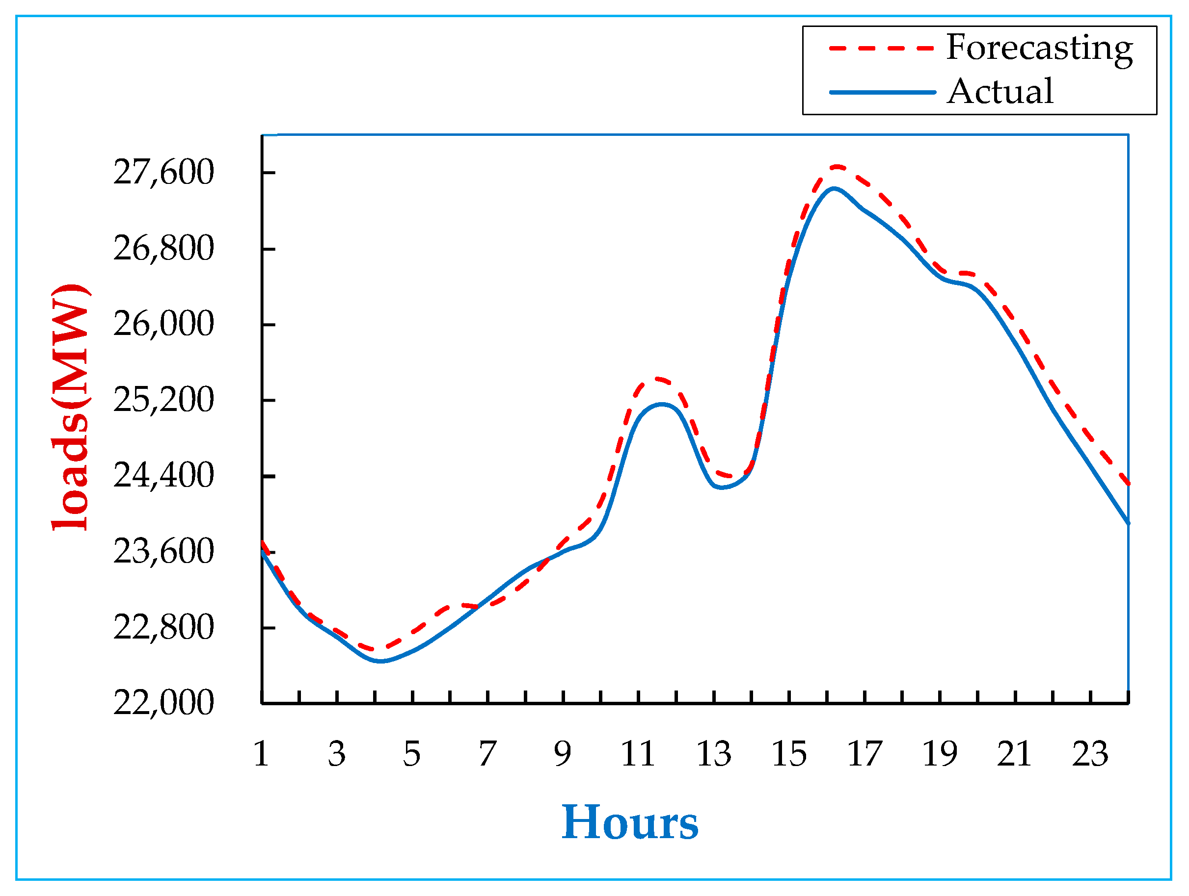
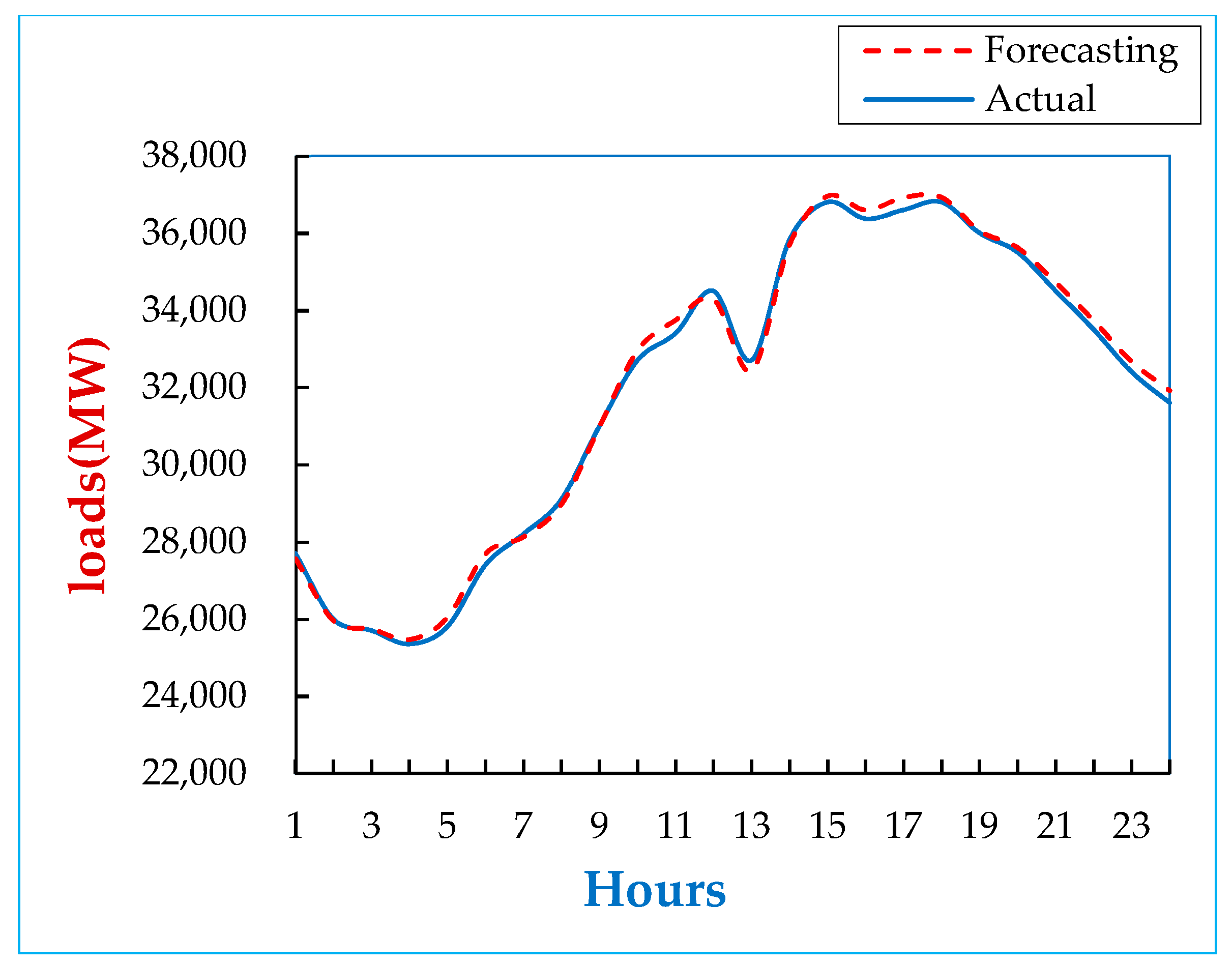
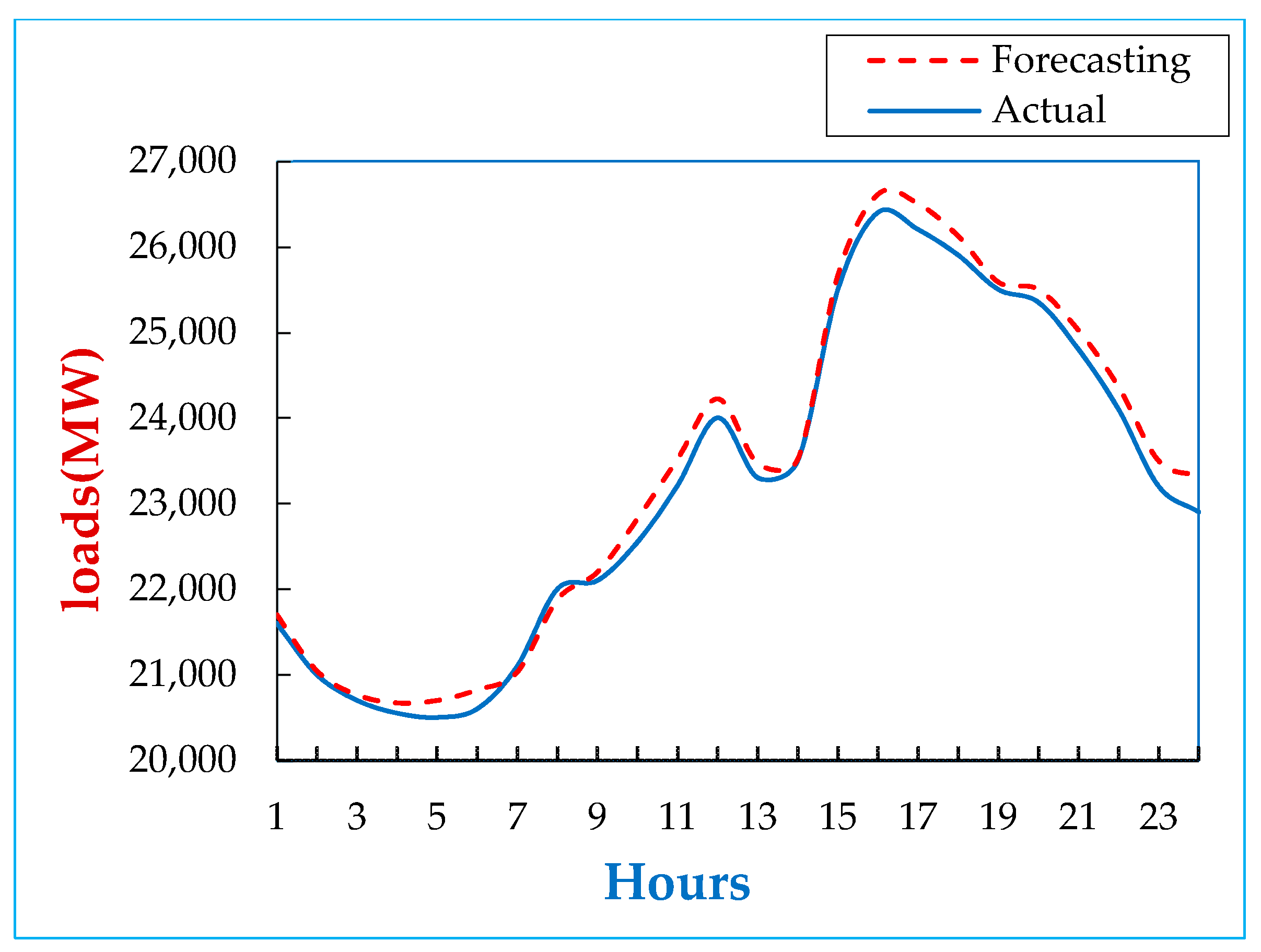
Usually, we perform the training work offline first and then go online to perform the actual forecasting work after the training is completed. The software used in this paper is Python 3.8. The training data used in this example are all data for the period from 12 March 2019 to 11 March 2020. The test data are from 10 May 2020 to 9 June 2020, and the actual forecasting for the load is from 1 January 2020 to 31 December 2020. CSSA (at the beginning, CSSA n = 30, D = 75) is used to search for the optimal values for network parameters for LSTM-NN, while LSTM-NN performs load forecasting of LSTM-NN after receiving the solution parameter values sent from CSSA training. In Figure 4, Figure 5 and Figure 6, the load forecasting graph for the actual date is used. In each figure, the solid line represents the actual load, and the dotted line represents the forecasted load. Shown in Figure 4 is the load forecasting for Monday, 7 September with a minimum load (22,571 MW) at about 4:00 a.m. and a maximum load (27,615 MW) at about 4:00 p.m. Shown in Figure 5 is the load forecasting for Wednesday, 16 September with a minimum load (25,470 MW) at about 4:00 a.m. and a maximum load (36,959 MW) at about 3:00 p.m. Moreover, shown in Figure 6 is a week-long holiday; on Saturday, 17 October, the curve in the figure shows that its load value is smaller than the typical working day, and the lowest load occurs at 4:00 a.m. (20,671 MW), while the maximum load (26,615 MW) is around 4:00 p.m.
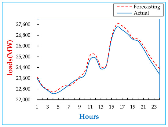
Figure 4.
Load forecasting results for working days (Monday, 7 September 2020).
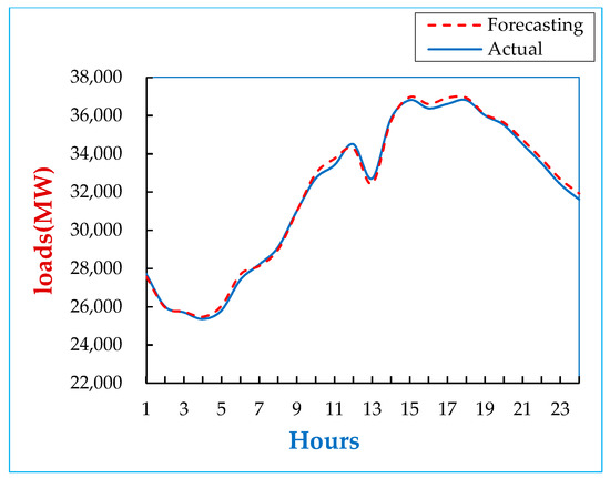
Figure 5.
Load forecasting results for working days (Wednesday, 16 September 2020).
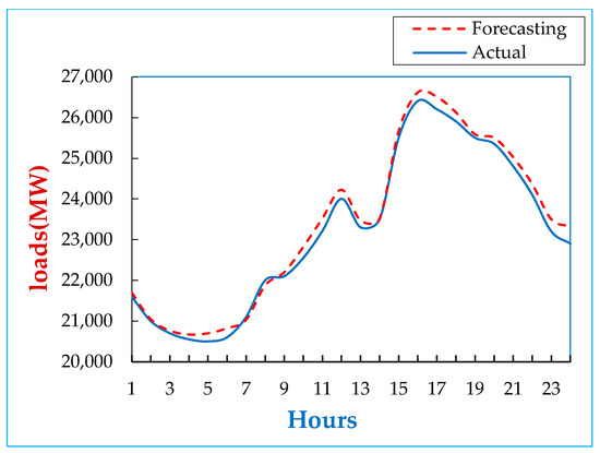
Figure 6.
Load forecasting results for a week-long holiday (Saturday, 17 October 2020).
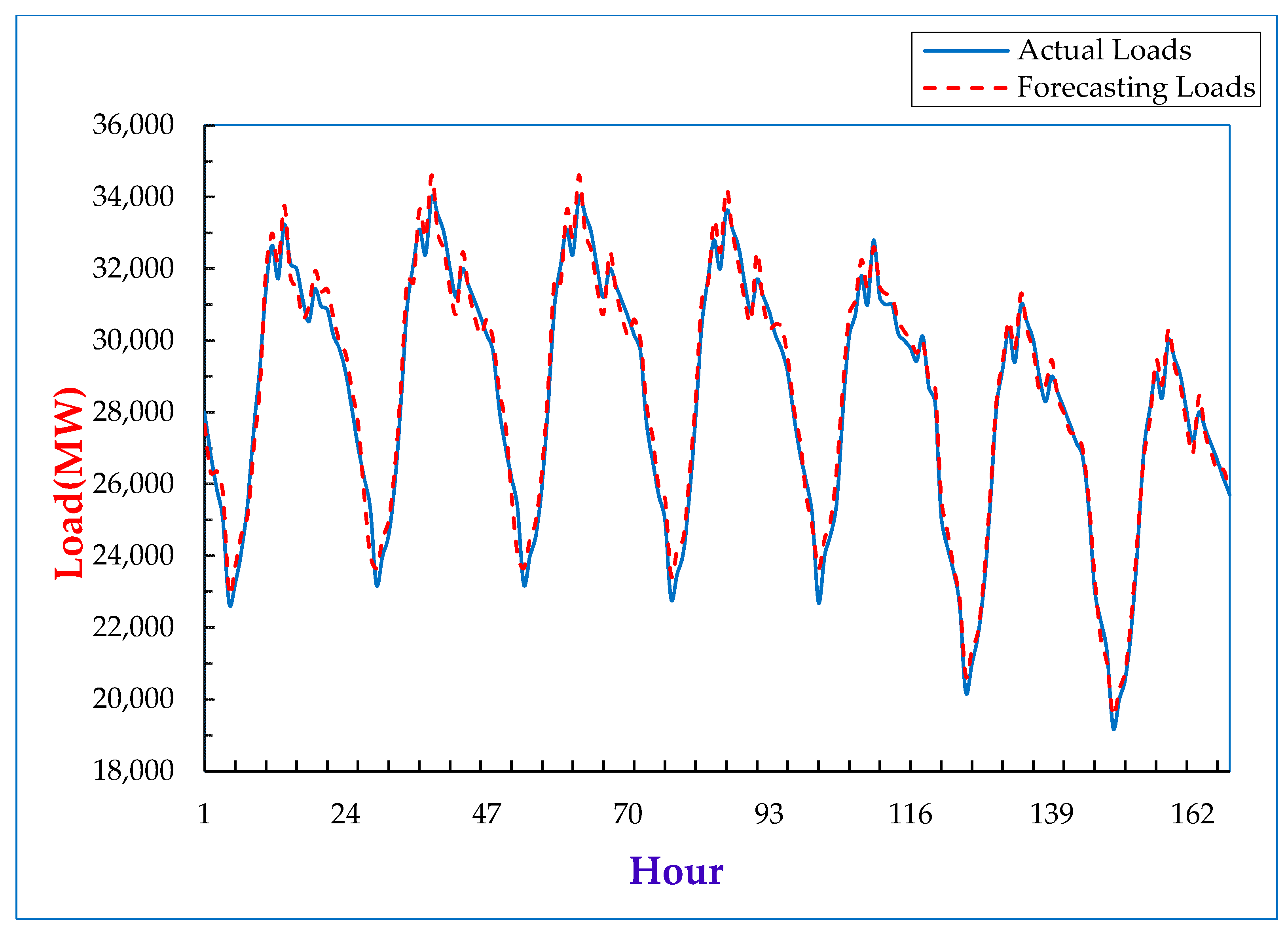
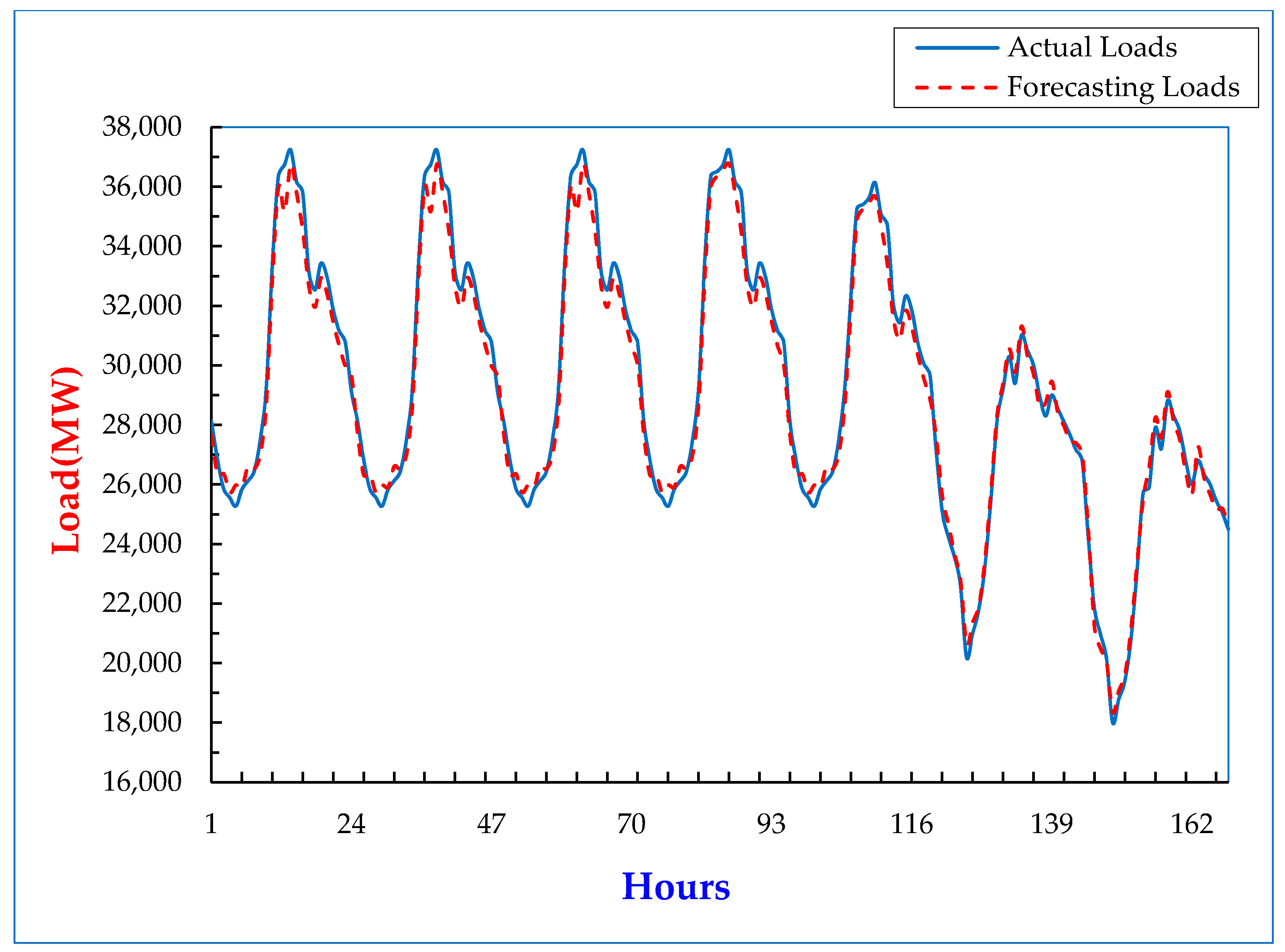
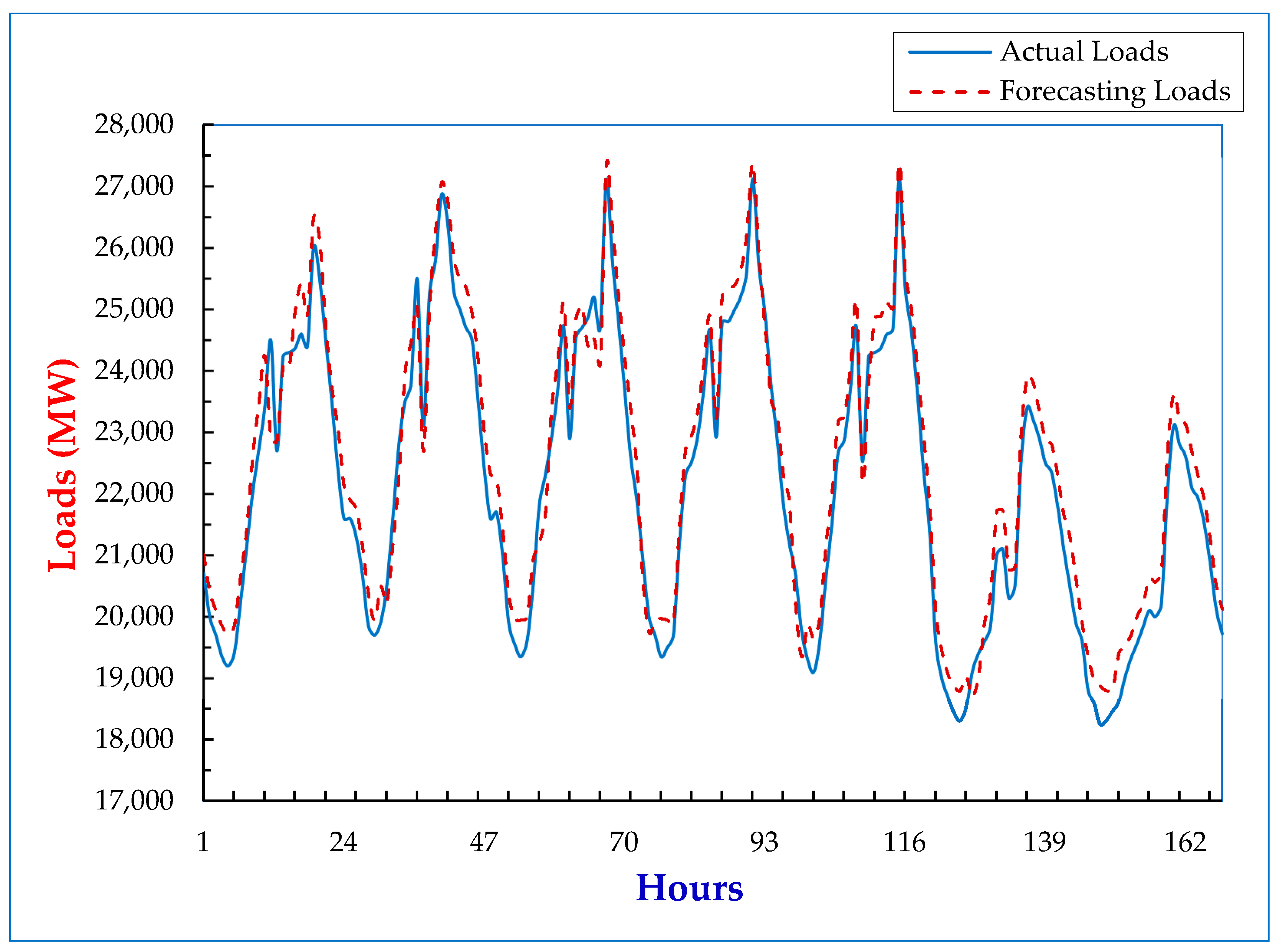
Furthermore, the load graph shown in Figure 7 is a load forecasting for the typical spring week of 2020 (Monday 11 May 2020 to Sunday 17 May 2020). The peak load of the typical weekly load forecasting is about 34,200 MW, and the point at which the daily peak load occurs is slightly different. Figure 8 is load forecasting for the typical summer week of 2020 (Monday 20 July 2020 to Sunday 26 July 2020). The peak load of the typical weekly load forecasting is about 37,235 MW. Finally, in Figure 9, the load graph is a load forecasting for the typical autumn week of 2020 (Monday 21 September 2020 to Sunday 27 September 2020). The peak load of the typical weekly load forecasting is about 27,350 MW.

Figure 7.
Load forecasting for the typical 2020 spring week (Monday 11 May 2020 to Sunday 17 May 2020).
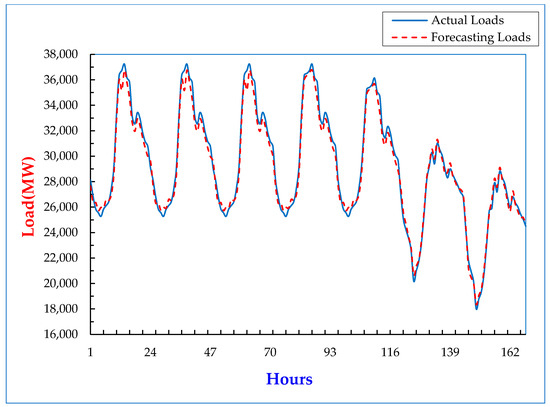
Figure 8.
Load forecasting for the typical 2020 summer week (Monday 20 July 2020 to Sunday 26 July 2020).
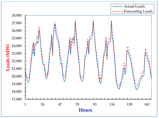
Figure 9.
Load forecasting for the typical 2020 autumn week (Monday 21 September 2020 to Sunday 27 September 2020).
8.2. Load Forecasting of Different Methods of Different Dates then Obtaining MAPE and Max MAPE
In this paper, the MAPE and Max. MAPE obtained from different day patterns can be predicted using different methods:
- ANN: Artificial Neural Network method.
- EP-ANN: With ANN as the main body of the forecasting model, and uses Evolutionary Programming (EP) to train its parameters.
- GA-LSTM: With LSTM as the main body of the forecasting model, and uses Genetic Algorithm (GA) to train its parameters.
- PSO-LSTM: With LSTM as the main body of the forecasting model, and uses Particle Swarm Optimization (PSO) to train its parameters.
- ILSTM-NN: The method used in this paper.
For all five methods, the total unit of input layers in this paper is 10. As shown in Table 1, in the case of working days, the value calculated using the ILSTM-NN method is different from ANN, EP-ANN, GA-LSTM, and PSO-LSTM; the calculated values were reduced (improved) by 55%, 43%, 36%, and 21%, respectively. In the case of non-working days, the values calculated using the ILSTM-NN method are lower than ANN, EP-ANN, GA-LSTM, and PSO-LSTM; the values calculated from the other four methods decreased (improved) by 33%, 31.4%, 20.4%, and 9.2%, respectively. For example, in the case of public holidays, the value calculated using the ILSTM-NN method is 33.3%, 27.4%, 22.2%, and 16.1% lower (improved) than the values calculated by ANN, EP-ANN, GA-LSTM, and PSO-LSTM, respectively. In the case of rainy days, the MAPE value calculated using the ILSTM-NN method is lower than ANN, EP-ANN, GA-LSTM, and PSO-LSTM by 31%, 29.2%, 24.3%, and 16.5%, respectively. Finally, if calculated in terms of the average for different day patterns, the average calculated using the ILSTM-NN method, compared to ANN, EP-ANN, GA-LSTM, and PSO-LSTM, improved by 49%, 41%, 30%, and 22%, respectively. In terms of ten average RMSE, the average RMSE calculated using the ILSTM-NN method, compared to ANN, EP-ANN, GA-LSTM, and PSO-LSTM, improved by 52.1%, 49.5%, 49.5%, and 44.1%, respectively.

Table 1.
A comparison of the load forecasting error values (, Max. , and RMSE) for different dates by different methods from 5 July to 20 October 2020.
Regarding the monthly differences for and Max. , the averages obtained using different methods for the whole year from January 2020 to December 2020 are shown in Table 2. From the table observations, almost every different method is calculated in the summer (June, July, August, etc.) when the average values of and Max. are higher than in the other months. This result is primarily due to the more volatile weather conditions in the summer, as typhoons are common in Taiwan during the summer months. On the other hand, because electricity consumption in hot weather often constitutes record-breaking annual electricity consumption, these factors are the main reasons for the higher error value of load forecasting. As shown in Table 3, the different and Max. between the hours measured at different points in time within 24 h of the “working day” (Thursday 15 October 2020) are calculated using different methods listed in Table 1. Each hour calculated at different points in time is different, including and Max. . Observable from the table, using the ILSTM-NN method, the sum of Max. and per hour calculated by the method are smaller than the values calculated by the other four methods. The average value calculated using the ILSTM-NN method is lower than ANN, EP-ANN, GA-LSTM, and PSO-LSTM by 53.1%, 50.0%, 47.6%, and 36.5%, respectively.
Table 2.
The average and Max. of each month was obtained using different methods for different months, from 1 January 2020 to 20 December 2020.
Table 3.
Different methods used to measure the difference between Max and .. Meanwhile, the hours are measured at different time points within 24 h of the “working day” (Thursday 15 October 2020) in Table 1.
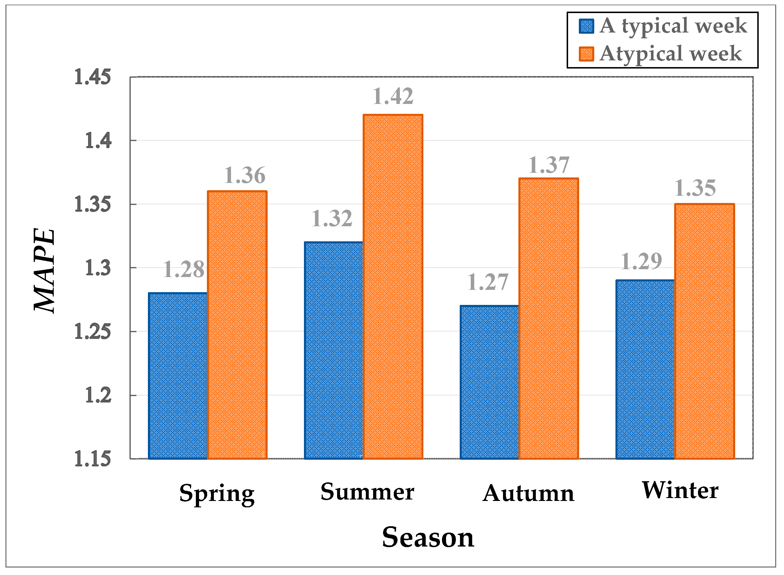
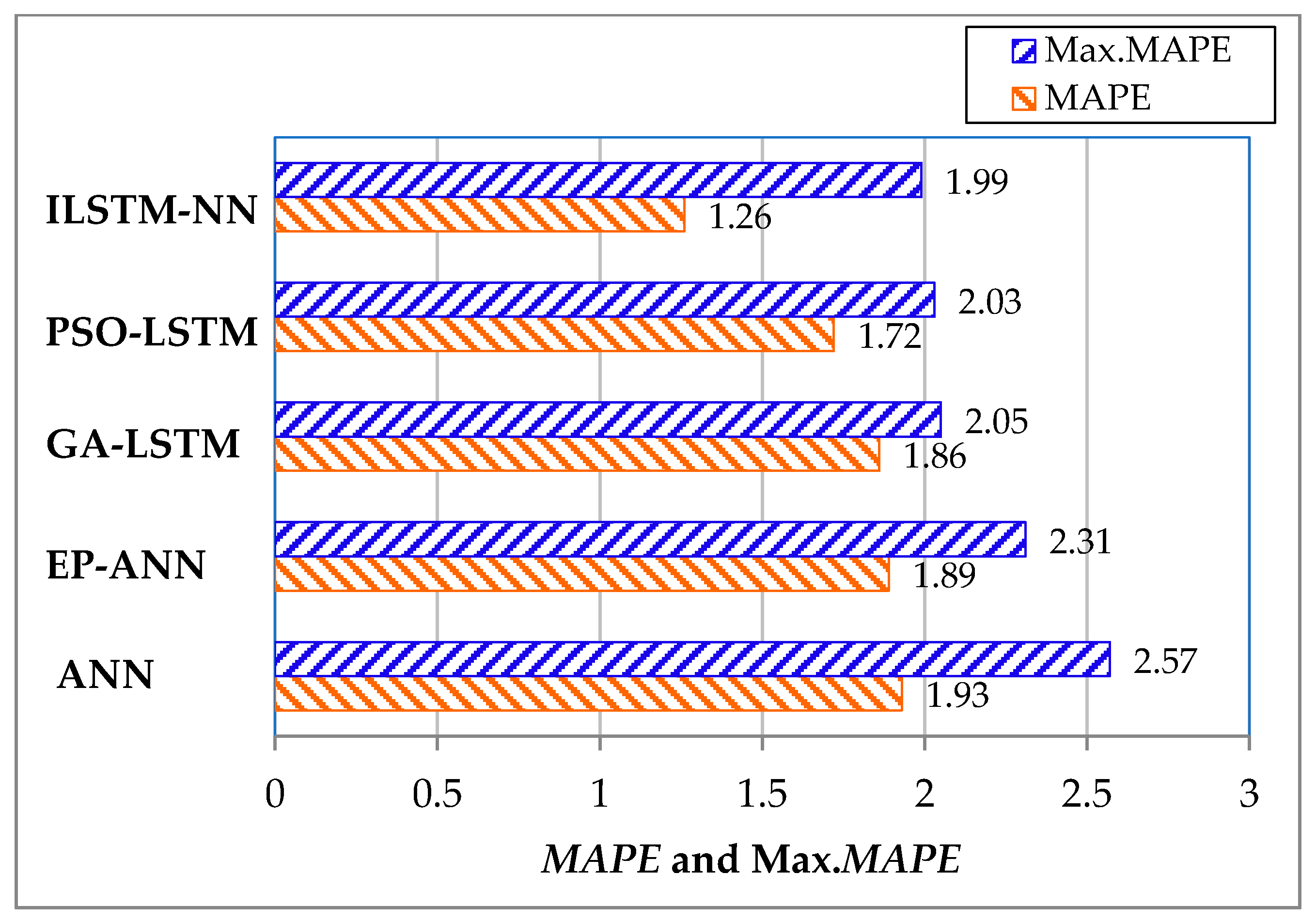
Shown in Figure 10 are the four seasons of 2020 (spring, summer, autumn, winter) calculated using the ILSTM-NN method. Comparing average load forecasting for a typical week and an atypical week, as seen from the four seasons, the value measured in summer is higher than the load forecasting for the other three seasons. The value in summer is approximately 3%, 3.9%, and 2.3% higher than in spring, autumn, and winter. Furthermore, Max. in summer is higher than spring, autumn, and winter by approximately 4.4%, 3.6%, and 5.2%, respectively. (The atypical week refers to the week when there are rainy days, typhoon days, etc.) As shown in Figure 11, the load forecasting Max. for a working day (Thursday 2020/10/15) is compared with the other four methods, ANN, EP-ANN, GA-LSTM, and PSO-LSTM, and its improvement values are about 29%, 16%, 3%, and 2%, respectively.

Figure 10.
A comparison of , a typical week and an atypical week’s average load forecast for the four seasons of 2020.
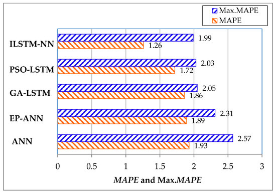
Figure 11.
The and Max. of the load forecasting for a particular working day (Thursday 15 October 2020) compared with the other four different methods.
9. Conclusions
The current short-term load forecasting model cannot handle complex nonlinear loads and the hidden deep relationships between data, resulting in the model’s subpar forecasting accuracy. In this paper, a solution to improve the LSTM-NN method for short-term load forecasting is proposed for the complexity of the power system. The CSSA method was used here to adjust the parameter values of LSTM-NN. CSSA’s superior search ability can determine the optimal parameters of LSTM-NN, and thus, we can use the LSTM-NN to generate the optimal solution of load forecasting. The advantages of CSSA include that (1) there are not many parameters to adjust, and that (2) it does not fall into the trap of finding locally optimal solutions to problems, instead finding the globally optimal solution. The improved LSTM-NN is applied to the actual load forecasting for a region. Based on our data, the average is only about 2.6% to 2.8%. Compared with several other methods used usually for load forecasting (ANN, EP-ANN, GA-LSTM, and PSO-LSTM), the improved LSTM-NN significantly decreased (improved) the by nearly 20% to 50%, and the average RMSE decreased (improved) by nearly 44.1% to 52.1%. The superiority and practicability of this method are clearly demonstrated in this work, rendering the improved LSTM-NN ideal for practical complex load forecasting.
Funding
This research received no external funding.
Data Availability Statement
The data source can refer to the electricity consumption data of Kaohsiung, Taiwan.
Conflicts of Interest
The author declares no conflict of interest.
References
- Haida, T.; Muto, S. Regression-based peak load forecasting using a transformation technique. IEEE Trans. Power Syst. 1994, 9, 1788–1794. [Google Scholar] [CrossRef]
- Chen, J.; Wang, W.; Huang, C. Analysis of an adaptive time-series autoregressive moving-average (ARMA) model for short-term load forecasting. Elect. Power Syst. Res. 1995, 34, 187–196. [Google Scholar] [CrossRef]
- Charytoniuk, W.; Chen, M.S.; Van Olinda, P. Nonparametric regression-based Short-term load forecasting. IEEE Trans. Power Syst. 1998, 13, 725–730. [Google Scholar] [CrossRef]
- Amjady, N. Short-Term hourly load forecasting using time-series modeling with peak load estimation capability. IEEE Trans. Power Syst. 2001, 11, 498–505. [Google Scholar] [CrossRef]
- AI-Hamadi, H.M.; Soliman, S.A. Short-Term electric load forecasting based on Kalman filtering algorithm with moving window weather and load model. Electr. Power Syst. Res. 2004, 68, 47–59. [Google Scholar] [CrossRef]
- Mastorocostas, P.A.; Theochairs, J.B.; Bakirtzis, A.G. Fuzzy modeling for short-term load forecasting using the orthogonal least squares method. IEEE Trans. Power Syst. 1999, 14, 29–36. [Google Scholar] [CrossRef]
- Sholahudin, S.; Han, H. Simplified dynamic neural networks model to predict heating load of the building using Taguchi method. Energy 2016, 115, 1919–1926. [Google Scholar] [CrossRef]
- Liao, G.C. Hybrid Improved Differential Evolution and Wavelet Neural Networks with Load Forecasting Problem of Air Conditioning. Int. J. Electr. Power Energy Syst. 2014, 61, 673–682. [Google Scholar] [CrossRef]
- Niu, D.; Wang, Y.; Wu, D.D. Power Load Forecasting Using Support Vector Machine and Ant Colony Optimization. Expert Syst. Appl. 2010, 37, 2531–2539. [Google Scholar] [CrossRef]
- Yang, A.; Li, W.; Yang, X. Short-Term electricity load forecasting based on feature selection and Least Squares Support Vector Machines. Konwl. -Based Syst. 2019, 163, 159–173. [Google Scholar] [CrossRef]
- Xuan, Y.; Si, W.; Zhu, J.; Sun, Z.; Zhao, J.; Xu, M.; Xu, S. Multi-Model Fusion Short-Term Load Forecasting Based on Random Forest Feature Selection and Hybrid Neural Network. IEEE Access 2021, 9, 69002–69009. [Google Scholar] [CrossRef]
- Long, Y.; Su, Z.; Wang, Y. Monthly load forecasting model based on seasonal adjustment and BP neural network. Syst. Eng. Theory Pract. 2018, 38, 1052–1060. [Google Scholar]
- Feng, T.; Zhang, J. Assessment of aggregation strategies for machine-learning-based short-term load forecasting. Electr. Power Syst. Res. 2020, 184, 106304. [Google Scholar] [CrossRef]
- Khwaja, A.S.; Anpalagan, A.; Naeem, M.; Venkatesh, B. Joint bagged-boosted artificial neural networks: Using ensemble machine learning to improve short-Term electricity load forecasting. Electr. Power Syst. Res. 2020, 13, 1630–1637. [Google Scholar] [CrossRef]
- Mehedi, I.M.; Bassi, H.; Rawa, M.J.; Ajour, M.; Abusorrah, A.; Vellingiri, M.T.; Salam, Z.; Abdullah, P.B. Intelligent Machine Learning with Evolutionary Algorithm based Short Term Load Forecasting in Power System. IEEE Access 2021, 9, 100113–100124. [Google Scholar] [CrossRef]
- Hossen, T.; Plathottam, S.J.; Angamuthu, R.K.; Ranganathan, P.; Salehfar, H. Short-term load forecasting using deep neural networks (DNN). In Proceedings of the North American Power Symposium (NAPS), Morgantown, WV, USA, 17–19 September 2017; pp. 1–6. [Google Scholar]
- Ryu, S.; Noh, J.; Kim, H. Deep neural network-based demand side short term load forecasting. Energies 2017, 10, 3. [Google Scholar] [CrossRef]
- Zang, H.; Cheng, L.; Ding, T.; Cheung, K.W.; Liang, Z.; Wei, Z.; Sun, G. Hybrid method for short-Term photovoltaic power forecasting based on deep convolutional neural network. IET Gener. Transm. Distrib. 2018, 12, 4557–4567. [Google Scholar] [CrossRef]
- Rafi, S.H.; Masood, N.A.; Deeba, S.R.; Hossain, E. A Short-Term Load Forecasting Method Using Integrated CNN and LSTM and Network. IEEE Access 2021, 9, 32436–32448. [Google Scholar] [CrossRef]
- Deng, Z.; Wang, B.; Xu, Y.; Xu, T.; Liu, C.; Zhu, Z. Multi-scale convolutional neural network with time-cognition for multi-step short-term load forecasting. IEEE Access 2019, 7, 88058–88071. [Google Scholar] [CrossRef]
- Yin, L.; Xie, J. Multi-temporal-spatial-scale temporal convolution network for short-term load forecasting for power systems. Appl. Energy 2021, 283, 116328. [Google Scholar] [CrossRef]
- Tang, X.; Dai, Y.; Wang, T.; Chen, Y. Short-Term power load forecasting based on multi-layer bidirectional recurrent neural network. IET Gener. Transm. Distrib. 2019, 13, 3847–3854. [Google Scholar] [CrossRef]
- Tang, X.L.; Dai, Y.Y.; Liu, Q.; Dang, X.Y.; Zhao, J.; Xu, J. Application of bidirectional recurrent neural networks for short-Term and medium-term load forecasting. IEEE Access 2019, 7, 160660–160670. [Google Scholar] [CrossRef]
- Eskandari, H.; Imani, M.; Moghaddam, M.P. Convolutional and recurrent neural network based model for short-term load forecasting. Electr. Power Syst. Res. 2021, 195, 107173. [Google Scholar] [CrossRef]
- Wang, Y.; Gan, D.; Sun, M.; Zhang, N.; Lu, Z.; Kang, C. Probabilistic individual load forecasting using pinball loss guided LSTM. Appl. Energy 2019, 235, 11–20. [Google Scholar] [CrossRef] [Green Version]
- Tian, C.; Ma, J.; Zhang, C.; Zhan, P. A deep neural network model for short-term load forecasting based on Long Short-Term Memory Network and convolutional neural network. Energies 2018, 11, 3493. [Google Scholar] [CrossRef] [Green Version]
- Kong, W.; Dong, Z.Y.; Jia, Y.; Hill, D.J.; Xu, Y.; Zhang, Y. Short-Term Residential Load Forecasting Based on LSTM Recurrent Neural Network. IEEE Trans. Smart Grid 2019, 10, 841–851. [Google Scholar] [CrossRef]
- Pei, S.; Qin, H.; Yao, L.; Liu, Y.; Wang, C.; Zhou, J. Multi-Step Ahead short-term load forecasting Using Hybrid Feature Selection and Improved Long Short-Term Memory Network. Energies 2020, 13, 4121. [Google Scholar] [CrossRef]
- Santra, A.S.; Lin, J.L. Integrating Long Short-Term Memory and Genetic Algorithm for short-term load forecasting. Energies 2019, 12, 2040. [Google Scholar] [CrossRef] [Green Version]
- Ceperic, E.; Ceperic, V.; Baric, A. A Strategy for short-term load forecasting by Support Vector Regression Machines. IEEE Trans. Power Syst. 2013, 28, 4356–4364. [Google Scholar] [CrossRef]
- Hong, W.C. Chaotic Particle Swarm Optimization Algorithm in a Support Vector Regression Electric Load Forecasting Model. Energy Convers. Manag. 2009, 50, 105–117. [Google Scholar] [CrossRef]
- Vrablecova, P.; Bou Ezzeddine, A.; Rozinajova, V.; Sarik, S.; Sangaiah, A.K. Smart grid load forecasting using online support vector regression. Comput. Electr. Eng. 2018, 65, 102–117. [Google Scholar] [CrossRef]
- Jiang, H.; Zhang, Y.; Muljadi, E.; Zhang, J.J.; Gao, D.W. A Short-term and high-resolution distribution system load forecasting approach using support vector regression with hybrid parameters optimization. IEEE Trans. Smart Grid 2018, 9, 3341–3350. [Google Scholar] [CrossRef]
- Pan, E.; Mei, X.; Wang, Q.; Ma, Y.; Ma, J. Spectral-spatial classification for hyperspectral image based on a single GRU. Neurocomputing 2020, 387, 150–160. [Google Scholar] [CrossRef]
- Sajjad, M.; Khan, Z.A.; Ullah, A.; Hussain, T.; Ulah, W.; Lee, M.Y.; Baik, S.W. A novel CNN-GRU-based hybrid approach for short-term residential load forecasting. IEEE Access 2020, 8, 143759–143768. [Google Scholar] [CrossRef]
- Li, W.; Logenthiran, T.; Woo, W.L. Multi-GRU prediction system for electricity generation’s planning and operation. IET Gener. Transmiss. Distrib. 2019, 13, 1630–1637. [Google Scholar] [CrossRef]
- Li, G.; Hu, T.; Bai, D. BP Neural Network Improved by Sparrow Search Algorithm in Predicting Debonding Strain of FRP-Strengthened RC Beams. Adv. Civ. Eng. 2021, 2021, 9979028. [Google Scholar] [CrossRef]
- Liang, Q.; Chen, B.; Wu, H.; Ma, C.; Li, S. A Novel Modified Sparrow Search Algorithm with Application in Side Lobe Lobe Level Reduction of Linear Antenna Array. Wirel. Commun. Mob. Comput. 2021, 2021, 9915420. [Google Scholar] [CrossRef]
- Ouyang, C.; Qiu, Y.; Zhu, D. Adaptive Spiral Flying Sparrow Search Algorithm. Sci. Program. 2021, 2021, 6505253. [Google Scholar] [CrossRef]

Publisher’s Note: MDPI stays neutral with regard to jurisdictional claims in published maps and institutional affiliations. |
© 2021 by the author. Licensee MDPI, Basel, Switzerland. This article is an open access article distributed under the terms and conditions of the Creative Commons Attribution (CC BY) license (https://creativecommons.org/licenses/by/4.0/).