Numerical Simulation of Low Salinity Water Flooding on Core Samples for an Oil Reservoir in the Nam Con Son Basin, Vietnam

Abstract

Low-salinity water flooding (LSWF) is environment-friendly and operates similarly to conventional waterflooding without the need for synthetic chemical materials. The application of LSWF makes sense in Vietnam as HC production has steadily declined since 2002, and the majority of main oil fields have become near mature and mature fields. In the next years, Enhanced Oil Recovery (EOR) should be a top priority for Petro Vietnam to boost its oil production, for which the key issue is how to select a suitable EOR technology. In this study, LSWF of the Lower Miocene sand using low salinity water from Lower Oligocene sand was investigated. Previously at the Ruby field in the Cuu Long Basin, an LSWF feasibility study was carried out based on a conventional core flooding experiment, which is time-consuming and costly. This study targets the Chim Sao field in the Nam Con Son Basin, for which a cheaper and faster assessing method is required. As a result, a numerical code written in Matlab was developed and successfully validated with the core flooding experiment results obtained at the Ruby field. The LSWF simulation was conducted using the multiple ion-exchange mechanisms (MIE), and the results obtained showed an increase in the oil recovery factor by 2.19% for the Lower Miocene Sand. Another important outcome of this study is the innovative proposal and successful simulation to use the abundant low salinity water from the underlying Lower Oligocene sand as a natural LSW source to inject into the Lower Miocene oil reservoir that can be a decisive factor to help apply LSWF in practice on a wide scale not only for Chim Sao but also other similar oil fields in southern offshore Vietnam.

1. Introduction

For a long period since 1987, the main oil production of Vietnam has come from the famous White Tiger fractured granite reservoir in the Cuu Long Basin, which peaked in 2006 and then started to decrease gradually. On the other hand, contributions from the clastic Miocene and Oligocene reservoirs in the Cuu Long Basin and the Nam Con Son Basin become increasingly significant (see Figure 1). While the petroleum production from the Miocene sands is second to that from the fractured granite basement reservoirs since 2013, it also has started to reduce. The recovery factor of the Miocene reservoirs ranges from 15 to 35%. As a matter of fact, most major oil fields in Vietnam are in a declining phase, which requires an intensive study on Improved Oil Recovery (IOR) or Enhanced Oil Recovery (EOR) [1]

Thang et al. (2021) in [1] reported that many major oil fields in Vietnam are in the declining phase and can be classified as mature or near-mature fields, which need the application of IOR/EOR to sustain their production life. Thang and Giao (2017) [2] made an overview of EOR applications in Vietnam. Many studies related to the application of EOR using polymer, water—alternative—gas injection, thermally stable surfactant and nano-surfactant, namely [3,4,5,6], have been carried out. An EOR master plan was proposed based on a recent comprehensive study by Quy et al. 2020 [7], in which LSWF is considered as one of the viable methods, as shown in Figure 2 below:

The main objective of this study is to develop a numerical code in Matlab to simulate the 1D LSWF flooding process on core samples to investigate its feasibility in a mature oil field, i.e., the Chim Sao field, in the Nam Con Son Basin (see Figure 3a). The simulation in this study focused, however, only on the multiple ion exchange (MIE) mechanism so that the simulation results can be compared and validated by the laboratory core flooding experiment results obtained at the Ruby oil field in the Cuu Long Basin [8]. The scopes of this study include the followings: (i) performing a comprehensive overview of LSWF mechanisms and applications; (ii) screening and selection of a suitable study location in the Nam Con Son Basin; (iii) development of a one-dimensional numerical simulation of LSWF and validating it with the core flooding results from the Ruby field in the Cuu Long Basin, where an experimental study of LSWF was recently conducted using the conventional laboratory core flooding experiment; (iv) Performing a one-dimensional LSWF simulation using the newly developed code for the Lower Miocene sand using the natural low salinity water source from the below Oligocene sand for the Chim Sao oil field, the Nam Con Son Basin.

2. Overview of LSWF Mechanisms and Governing Equations

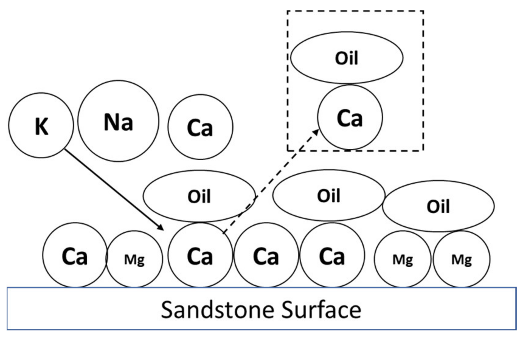
2.1. LSWF Mechanism

The mechanisms of LSWF have been studied in the laboratory scale more than two dedicates and can be classified as: (1) fines migration [9,10]; (2) mineral dissolution [11]; (3) increased pH effect and reduced interfacial tension [12]; (4) emulsification [8,13]; (5) multiple ion exchange [13,14,15]; (6) double-layer effects [16,17]; and (7) wettability alteration [18,19,20]. The following part will focus more on the multiple ion exchange (MIE) as one of the main mechanisms of LSWF employed in this study (see Figure 4), which is highly dependent on compositions of the formation water and injected brine. For LSWF to be effective, it is necessary for the formation (connate) water to contain sodium, calcium and magnesium ([13,14,15,21]). In an MIE process, the ions like K, Na will replace the divalent ions (e.g., Ca, Mg) that are adsorbed on the rock surfaces, leading to the liberation of oil in the form of calcium carboxylate complex (see Figure 4). In addition, the ion-exchange process explains why LSWF does not work when a core is acidized and fired when the cation exchange capacity (CEC) of the clay minerals is destroyed and why LSWF has little effect on refined oil because no polar compounds are present to strongly interact with the clay minerals ([16]).

An important observation reported from core flooding experiments, and field implementations ([22,23,24]) is that the effluent pH tends to increase during LSWF. This phenomenon can be explained by the dissolution of carbonate minerals, such as calcite and dolomite. Ionic exchange during LSWF leads to the adsorption of divalent ions (Ca²⁺, Mg²⁺) and promotes mineral dissolution, which provides further calcium and magnesium for ion exchange. This explanation is consistent with the results of Evje and Hiorth in 2011 [25] and Hiorth et al. 2010 [26].

2.2. LSWF Governing Equations

Integrated simulation of geochemical reactions and fluid flow with active ions in the porous media, especially LSWF for EOR, is essential for understanding the behavior of each chemical component in the fluid. PhreeQC, a USGS’s geochemical reaction package [28], can help simulate various geochemical processes, including equilibrium between water and minerals, ion exchangers, surface complexes, solid solutions, and gases. Consequently, PhreeQC can be used to couple with the other multiphase flow source codes, one of which is the Matlab reservoir simulation toolbox (MRST) developed by SINTEF to prototype new models and computational methods for reservoir simulation [29].

In this study, first, the black-oil model, as described by Bao et al. (2017) [30], is a special multicomponent, multiphase model with no diffusion among the fluid components. The name “black-oil” refers to the assumption that various hydrocarbon species can be lumped together to form two components at surface conditions and, namely, a heavy hydrocarbon component called “oil” and a light component called “gas.” At the reservoir conditions, these two components can be partially or completely dissolved in each other, depending on the pressure, forming a liquid oleic phase and a gaseous phase. In addition, there is an aqueous phase, which herein is assumed to consist of only water. Similar to the polymer model given by Bao et al. 2017 [30], the continuity equations for the LSWF model are given in the Equation (1) as follows:

$$\begin{gathered} \frac{\partial }{\partial t}\left({\rho }_{\alpha }\varphi s_{\alpha }\right)+\nabla .\left({\rho }_{\mathsf{\alpha }}{\mathit{v}}_{\alpha }\right)=0 \\ \frac{\partial }{\partial t}\left[{\rho }_w\varphi s_{w}c+{\rho }_r\left(1-{\varphi }_{ref}\right)\right]+\nabla .\left(c{\rho }_w{\mathit{v}}_w\right)=0 \end{gathered}$$

(1)

where: $\varphi$ is rock porosity; $s_{\alpha }, {\rho }_{\alpha }$ and ${\mathit{v}}_{\alpha }$ are saturation, density and velocity of phase $\alpha ,$ respectively; c is the concentration of a certain chemical component given in mass per volume of water; ${\varphi }_{ref}$ and ${\rho }_r$ are reference porosity and density of the rock.

The phase fluxes velocity, ${\mathit{v}}_{\alpha },$ are estimated from Darcy’s law given as follows:

$$v_{\alpha }=-{\lambda }_{\alpha }\mathit{K}\left(\nabla p_{\alpha }-{\rho }_{\alpha }g\nabla z\right), \alpha =o,w$$

(2)

where: K is absolute permeability of the reservoir rock; ${\lambda }_{\alpha }=\frac{k_{r\alpha }}{{\mu }_{\alpha }}$ is the mobility of phase $\alpha$; $k_{r\alpha }$ is relative permeability and ${\mu }_{\alpha }$ is the phase viscosity.

The fully implicit simulation with low and high order schemes have been proposed and solved Equations (1) and (2) by Bao et al. 2017 [30], and Mykkeltvedt et al. 2019 [31] and the finite volume method was used to solve numerically.

3. Numerical Simulation and Validation of LSW Core Flooding

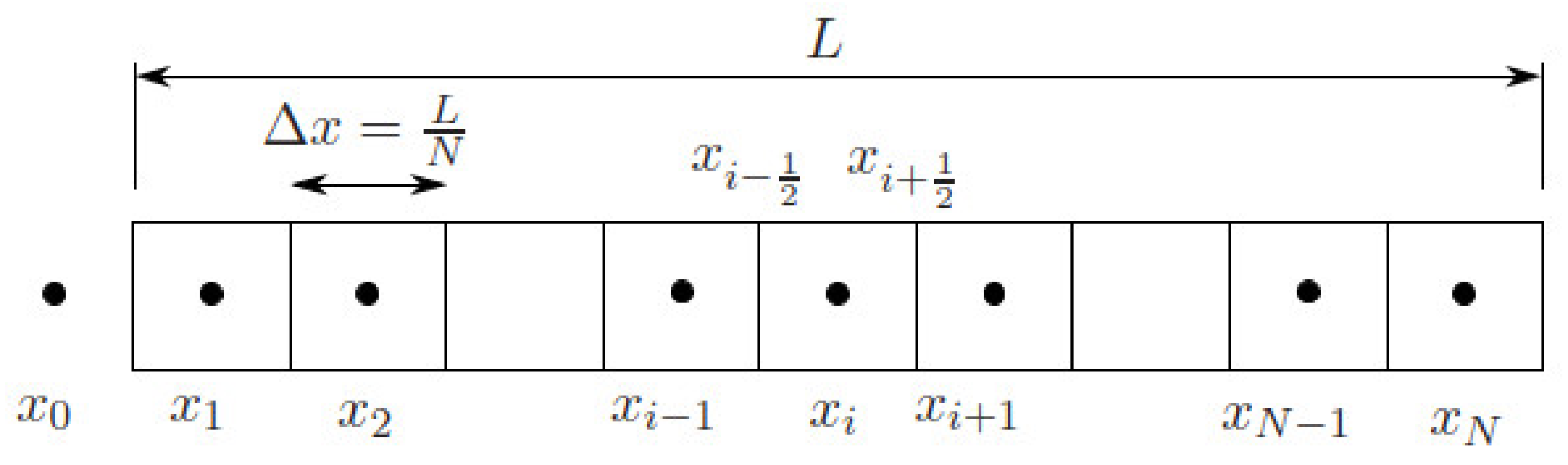
3.1. Finite Volume Formulation of Ion Transport Equation

To simulate an LSW core flooding experiment, a one-dimensional LSW flow model coupled with chemical reactions will be employed in this study. Figure 5 shows a finite volume (FV) discretization of the core with specified boundary conditions at the core end. The sequence of core flooding to be simulated include the followings steps: (i) First, (flow simulation), low salinity water is injected at a constant pressure higher than the reservoir pressure at the left end (x = 0), while at the right end (x = L) the pressure is kept constant as the reservoir pressure; (ii) Second, (simulation of occurring chemical reactions), the chemical reactions of transported ions of the formation (connate) water with the ions in the injected LS water will be simulated, and as the results, the salinity of the mixed fluid will be calculated, based on which the relative permeability of hydrocarbon will be determined as a function of salinity that is discussed in the literature by Shojaei et al. 2015 [32].

By using the 1D model and neglecting compressibility, we can rearrange the flow Equation (1) with chemical component transport in Buckley–Leverett form as follows:

$$\begin{gathered} \frac{\partial s_w}{\partial t}+\frac{v}{\varphi }\frac{\partial f_w}{\partial x}=0 \\ \frac{\partial \left(s_{w}c\right)}{\partial t}+\frac{v}{\varphi }\frac{\partial \left(f_{w}c\right)}{\partial x}=0 \end{gathered}$$

(3)

in which $f_w$ is the fractional flow, which is defined as:

$$f_w=\frac{{\lambda }_w}{{\lambda }_w+{\lambda }_o}+\frac{{\lambda }_w{\lambda }_o}{{\lambda }_w+{\lambda }_o}\frac{1}{v}\left(\Delta {\rho }_{wo}g\sin \left(\vartheta \right)+\frac{\partial p_c}{\partial x}\right)$$

(4)

where $p_c$ is the capillary pressure, $\Delta {\rho }_{wo}$ the density difference between water and oil, g the gravitational acceleration, $\vartheta$ the angle inclination of the reservoir. For the case of core flooding, the capillary pressure is negligible, and the core sample is placed horizontally, Equation (4) can be reduced to:

$$f_w=\frac{{\lambda }_w}{{\lambda }_w+{\lambda }_o}$$

(5)

The Buckley–Leverett equation is discretized in one-dimension space of length L with a mesh of N + 1 grid points $x_i$ for $i=0, 1, 2,\dots , N$ is shown in Figure 5. All grid cells have $\Delta x=l/N$ width and are of the cell-centered type.

Taking integration of Equation (3a) over a single grid cell, one gets:

$${{\displaystyle \int }}_{x_{i-\frac{1}{2}}}^{x_{i+\frac{1}{2}}}\frac{\partial s_w}{\partial t}dx=-\frac{v}{\varphi }{{\displaystyle \int }}_{x_{i-\frac{1}{2}}}^{x_{i+\frac{1}{2}}}\frac{\partial f_w}{\partial x}dx$$

(6)

that leads to

$$\frac{d}{dt}\left(\Delta x{s}_{w,i}\right)=-\frac{v}{\varphi }\left(f_{w,i+\frac{1}{2}}-f_{w,i-\frac{1}{2}}\right)$$

(7)

where $s_{w,i}$ is average water saturation at each grid cell $i.$

Using the first accurate Euler forward method for the left-hand side (LHS) of Equation (7), then for the spatial discretization, the first-order upwind is applied to get the fully explicit form of the water saturation as follows:

$$s_{w,i}^{n+1}=s_{w,i}^n-\frac{v}{\varphi }\frac{\Delta t}{\Delta x}\left(f_{w,i}-f_{w,i-1}\right)$$

(8)

In the matrix form, Equation (8) is written as follows:

$${\mathit{s}}_{\mathit{w}}^{\mathit{n}+\mathit{1}}={\mathit{s}}_{\mathit{w}}^{\mathit{n}}-\frac{v}{\varphi }\frac{\Delta t}{\Delta x}\left({\mathit{K}}_{\mathit{v}}{\mathit{f}}_{\mathit{w}}^{\mathit{n}}-{\mathit{f}}_{\mathit{b}\mathit{c}}^{\mathit{n}}\right)$$

(9)

where ${\mathit{s}}_{\mathit{w}}^{\mathit{n}}$ is $N\times 1$ vector of the water saturation of all grid cells at a time step $n$; ${\mathit{K}}_{\mathit{v}}$ is $N\times N$ matrix that is defined as follows:

$${\mathit{K}}_v=\left(\begin{array}{ccc}1& & \\ -1& 1& \\ & \ddots & \ddots \\ & -1& 1\end{array}\right)$$

(10)

and ${\mathit{f}}_{\mathit{w}}^{\mathit{n}}$ and ${\mathit{f}}_{\mathit{b}\mathit{c}}^{\mathit{n}}$ are $N\times 1$ vectors given as:

$${\mathit{f}}_{\mathit{w}}^{\mathit{n}}=\left(\begin{array}{c}{f}_{w,1}^n\\ \begin{array}{c}{f}_{w,2}^n\\ ⋮\\ ⋮\end{array}\\ f_{w,N}^n\end{array}\right),\hspace{1em}{\mathit{f}}_{\mathit{b}\mathit{c}}^n=\left(\begin{array}{c}{f}_{w,0}^n\\ \begin{array}{c}0\\ ⋮\\ ⋮\end{array}\\ 0\end{array}\right)=\left(\begin{array}{c}1\\ \begin{array}{c}0\\ ⋮\\ ⋮\end{array}\\ 0\end{array}\right)$$

(11)

A second-order time discretization was introduced using the modified Euler method [33], which can capture both information at the beginning of a time step (equal to the Euler forward method) and the information at the end of a time step. Additionally, this approximation also mitigates the small oscillations happened when the relative permeability curve switch at the shock front. Equation (9) can be rewritten according to the modified Euler method as follows [33]:

$${\mathit{s}}_{\mathit{w}}^{\mathit{n}+1}={\mathit{s}}_{\mathit{w}}^{\mathit{n}}-\frac{v}{\varphi }\frac{\Delta t}{\Delta x}\frac{\left({\mathit{K}}_{\mathit{v}}{\mathit{f}}_{\mathit{w}}^{\mathit{n}}-{\mathit{f}}_{\mathit{b}\mathit{c}}^{\mathit{n}}\right)+\left({\mathit{K}}_{\mathit{v}}{\tilde{\mathit{f}}}_{\mathit{w}}^{\mathit{n}+1}-{\mathit{f}}_{\mathit{b}\mathit{c}}^{\mathit{n}+\mathit{1}}\right)}{2}$$

(12)

where ${\tilde{\mathit{f}}}_{\mathit{w}}^{\mathit{n}+\mathit{1}}$ can be determined by first calculating the predictor step of water saturation, ${\tilde{\mathit{s}}}_{\mathit{w}}^{\mathit{n}+\mathit{1}}$ as given in Equation (9).

In fact, the above-mentioned modified Euler method is a special case of Runge–Kutta method for solving ODE (ordinary differential equations) [34]. For the single chemical component transport equation (Equation (3b)) by taking the derivative of a functioning product, Equation (3b) becomes:

$$\frac{\partial c}{\partial t}+\frac{v}{\varphi }\frac{f_w}{s_w}\frac{\partial c}{\partial x}=0$$

(13)

It is noted that, physically, the water saturation of each cell (S_w) is higher than that of the connate water saturation (S_wc), i.e., $s_w\ge s_{wc}>0$, so that Equation (15) is valid.

Theoretically, Equation (15) can be discretized in a similar way the Buckley–Leverett advection equation was done as mentioned above. A problem arising with first-order spatial discretization is that it often exhibits large numerical dispersion. Especially for multi tracers augmented reservoir simulation, this has been discussed in the works by Alsofi and Blunt (2010) [35], Jerauld et al. (2006 and 2008) [36,37]. In fact, one of the ways of limiting numerical dispersion is to increase the number of grid cells, which is often inapplicable as it leads to a very large amount of grid cells in augmented reservoir simulations. In order to overcome the dispersion in a first-order upwind system, the higher numerical schemes can be used while keeping the realistic amount of grid cells as given in the following equation [38]:

$$c_i^n=c_i^n-\frac{v\Delta t}{2\varphi \Delta x}\frac{f_{w,i}^n}{s_{w,i}^n} \left(3c_i^n-4c_{i-1}^n+c_{i-2}^n\right)$$

(14)

However, higher-order numerical schemes suffer from oscillation near discrete steps. That is, if one tries to simulate a slug of low salinity concentration with the numerical scheme from Equation (14) will be heavily distorted and lead to faulty conclusion and non-physical results [39].

The removal of oscillations from higher-order schemes can be done by using the so-called flux limiters [40]. The procedure consists of two steps. In the first step, the 2nd order upwind scheme is rewritten as a correction to the monotone first-order upwind difference and the correction term is written in the form of successive gradients as in the followings:

$$c_i^{n+1}=c_i^n-\stackrel{1st order upwind}{\overbrace{\frac{v\Delta t}{\varphi \Delta x}\frac{f_{w,i}^n}{s_{w,i}^n}\left[c_i^n-c_{i-1}^n\right]}}-\underset{Correction terms}{\underbrace{\frac{v\Delta t}{\varphi \Delta x}\frac{f_{w,i}^n}{s_{w,i}^n}\left[\frac{1}{2}\left(c_i^n-c_{i-1}^n\right)-\frac{1}{2}\left(c_{i-1}^n-c_{i-2}^n\right)\right]}}$$

(15)

In the second step, both non-monotonous terms are multiplied by the flux limiter functions $\mathsf{\Psi }\left(r_i\right)$ and $\mathsf{\Psi }\left(r_{i-1}\right)$ where

$$r_i=\frac{v_{i+1}-v_i}{v_i-v_{i-1}} \mathrm{and}{r}_{i-1}=\frac{v_i-v_{i-1}}{v_{i-1}-v_{i-2}}$$

(16)

and the flux limiter function can be one of three followings:

• Superbee: $\mathsf{\Psi }\left(r_i\right)=\max \left[0,\min \left(2r_i,1\right),\min \left(r_i,2\right)\right]$
• Minmod: $\mathsf{\Psi }\left(r_i\right)=\max \left[0,\min \left(r_i,1\right)\right]$ and
• Sweby: $\mathsf{\Psi }\left(r_i\right)=\max \left[0,\min \left(\beta r_i,1\right),\min \left(r_i,\beta \right)\right];\left(1\le \beta \le 2\right)$

which leads to

$$c_i^{n+1}=c_i^n-\frac{v\Delta t}{\varphi \Delta x}\frac{f_{w,i}^n}{s_{w,i}^n}\left[\left(1+\frac{1}{2}\mathsf{\Psi }\left(r_i\right)\right)\left(c_i^n-c_{i-1}^n\right)-\frac{1}{2}\mathsf{\Psi }\left(r_{i-1}\right)\left(c_{i-1}^n-c_{i-2}^n\right)\right]$$

(17)

There is no suitable flux limiter function for all cases. A full review of all mathematical requirements and their implementation is summarized by Hirsch, 2007 [40].

Equation (17) can now be fully solved numerically. However, it is still used for the first-order accuracy in the time domain. As second-order accuracy is desired, the same modified Euler method that was applied to solve Equation (3a) as mentioned above will be applied to Equation (17), and the final numerical prediction of a single time step, as shown in the following:

$$c_i^{n+1}=c_i^n-\frac{v\Delta t}{\varphi \Delta x}\frac{f_{w,i}^n}{s_{w,i}^n}\left[\left(1+\frac{1}{2}\mathsf{\Psi }\left(r_i\right)\right)\frac{\left(c_i^n-c_{i-1}^n\right)+({\tilde{c}}_i^n-{\tilde{c}}_{i-1}^n)}{2}-\frac{1}{2}\mathsf{\Psi }\left(r_{i-1}\right)\left(c_{i-1}^n-c_{i-2}^n\right)\right]$$

(18)

Stability conditions:

With the standard advection formula in the form of:

$$\frac{\partial u}{\partial t}+a\frac{\partial u}{\partial x}=0$$

(19)

the conversion criteria known as Courant–Friedrichs–Lewy (CFL) condition as described by Chen, 2008 [41], is given as follows:

$$\Delta t\le \frac{\Delta x}{a}$$

(20)

Consequently, for the case of the Buckley–Leverett equation (Equation (3a)), the derivative of the fractional flow with respect to the water saturation is maximum in order to satisfy the CFL condition, which means:

$$\Delta t_{BL}\le \frac{\varphi \Delta x}{v\max \left(\frac{d{f}_w}{d{s}_w}\right)}$$

(21)

For the cases of chemical components (ions) transport (equation 3b), the stability condition will be:

$$\Delta t_{it}\le \frac{\Delta t_{BL} \min \left(s_w\right) }{\max \left(f_w\right)}=\Delta t_{BL}\frac{s_{wc}}{1}$$

(22)

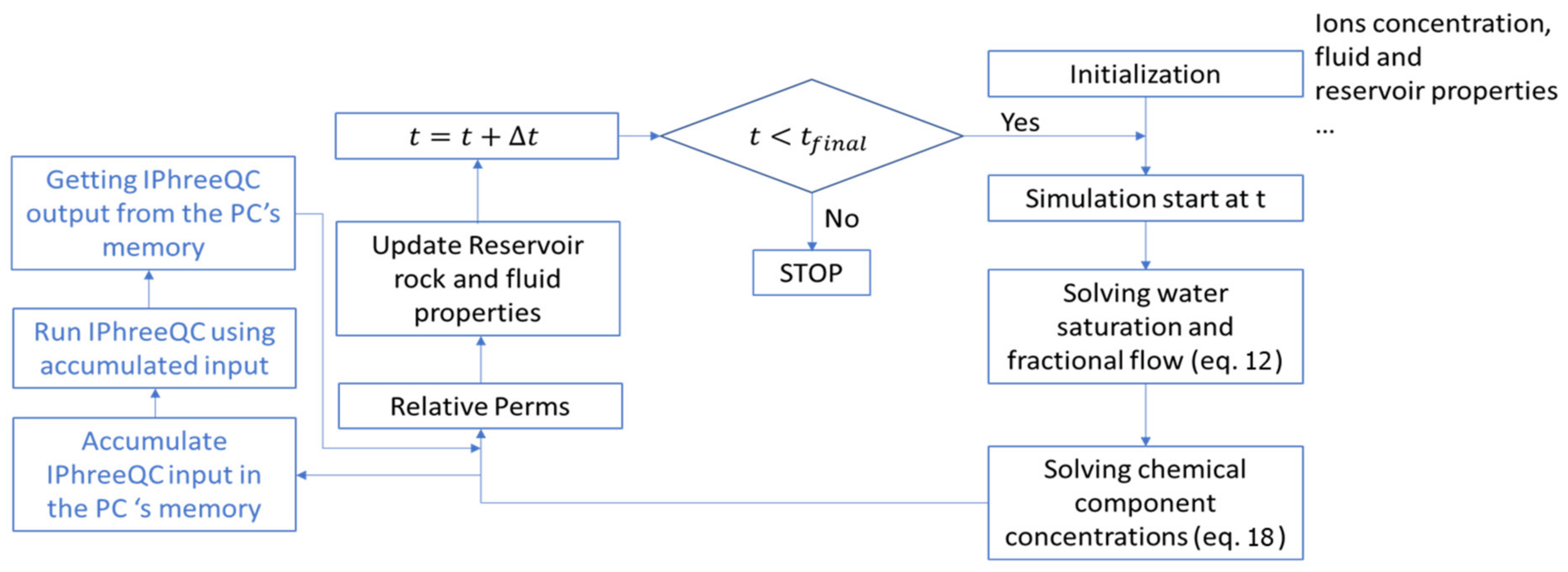
3.2. Coupling Chemical Component Transport with Chemical Reactions

Figure 6 shows the flowchart in this study to simulate the process of two-phase fluid transport with chemical reactions in a porous media that was used for simulating a core flooding experiment with constant porosity and permeability. In this workflow, the simulation starts at time t once the initialization is made. After this, the fractional flow (${\mathit{f}}_{\mathit{w}})$ and water saturation $({\mathit{s}}_{\mathit{w}})$ are implicitly solved by Equation (12), and the concentration equation of each chemical component will be further solved by Equation (18). When the concentrations of chemical components at a grid cell are calculated, they will be transferred to the IphreeQC [42], which is designed to increase the flexibility in interfacing with the widely used PhreeQC. Consequently, the newly obtained concentrations of these components/ions after chemical reactions will be compared with a certain salinity threshold to determine whether the injected water is of high or low salinity and to make the changes of relative permeability of water and oil as represented by Corey’s coefficient [43]. In the studies by Shojaei et al. 2015 [32]; Jerauld et al. 2008 [37] and Tripathi and Mohanty, 2008 [4], Corey’s coefficients ($n_o$) are a function of salinity, $X_c,$ but above a certain threshold of salinity (high salinity $X_c^{HS}$) and below a certain level of salinity (low salinity, $X_c^{LS}$) it has no salinity dependency as described below:

$$n_o\left(X_c\right)=n_o^{LS}+\frac{X_c-X_c^{Ls}}{X_c^{LS}-X_c^{HS}}\left(n_o^{LS}-n_o^{HS}\right)$$

(23)

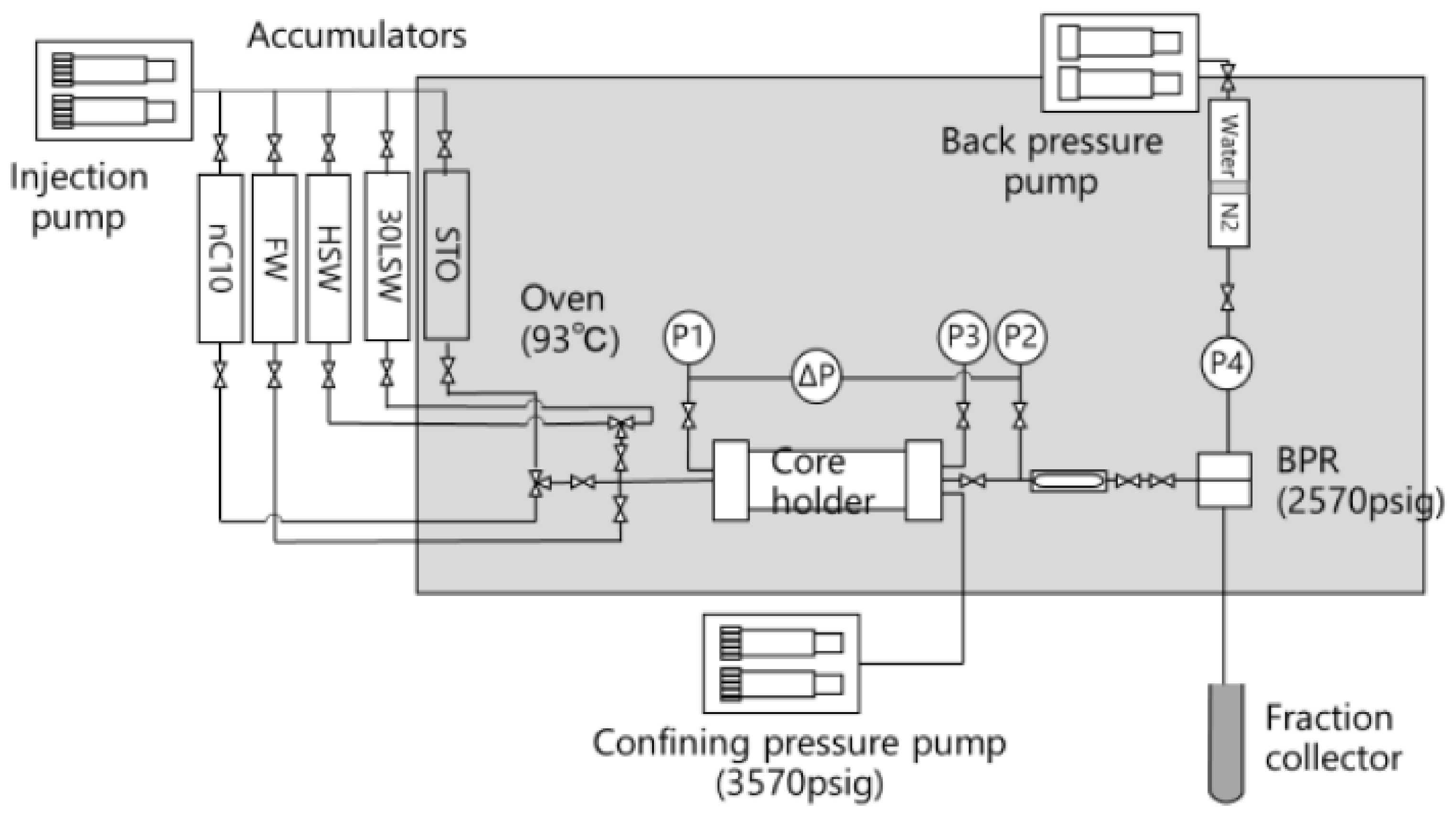
3.3. Validation of the LWSF Simulation Results with Those of a Core Flooding Experiment

Based on the FV formulation of equation 18 and its coupling with chemical reactions, as shown by the workflow in Figure 6, a fully functional code was developed in Matlab with IphreeQC functions being called via Com-server for the chemical reaction’s simulation to implement the simulation of LSW core flooding. To validate the new code, we used X_c^LS = 1000 ppm, X_c^HS = 7000 ppm for low and high salinity, respectively, following Tripathi and Mohanty’s (2008) model [44]. The validation of the new code was done by comparing the simulation results with those of a core flooding experiment conducted for the Ruby field in the Cuu Long Basin. The core sample and fluid properties and ion concentrations, including oil, high salinity (HS) and low salinity (LS) water, are presented in

Table 1. The petrophysical and physical properties of core samples and injected fluids.

Description	Variables	Unit	HS Value	LS Value
Porosity	ϕ	%	23.4	23.4
Absolute permeability	K	mD	500	500
Reservoir temperature	T	°C	93	93
Corey water coefficient	nw	-	2.5	2
Corey oil coefficient	no	-	3.5	3
Water viscosity	μw	cP	0.45	0.42
Oil viscosity	μo	cP	3.55	n/c
Initial water saturation	sw,init	%	50	50
Connate water saturation	sw,c	%	20	20
Residual oil saturation	sw,or	%	20	15

and

Table 2. Ion concentrations and physical properties of the formation water, high and low salinity water.

		FW	HS	LS
Density (g/cc)		0.996	0.987	0.972
Viscosity (cP)		0.45	0.45	0.42
Ion concentrations (ppm)	Na+	12,223	11,345	3782
	Ca2+	2133	441	14.7
	Mg2+	320	1075	35.8
	K+	137	439	14.6
	Cl−	23,159	19,835	661.2
	SO42−	72	2676	89.2
	PH	7.55	8.11	8.21
	Salinity	38,044	35,811	1194

. The core flooding experiment first started with HS water injection; after that, at a pore volume of 20 PV, an LS water will be injected. The setup of an LWS core flooding is shown in Figure 7 [8], in which the reservoir pressure (2570 psi) and temperature (93 °C) in an oven are kept constant. First, the cores were saturated with FW and cured for 7 days; then, the n-decane was injected until irreducible water saturation was achieved. In the next step, stock tank oil (STO) was injected until the n-decane was perfectly replaced, and the cores were cured by the STO for 40 days. The injection rate was 0.1 cc/min, equivalent to 1 ft/day of flow velocity in the reservoir. The stable outlet pressure of the core was controlled by using a back pressure regulator (BPR), and the differential pressure was measured from changes in the inlet and outlet pressure gauges. The recovered oil and effluent were collected at fixed intervals. After a flooding test, recovery was confirmed using a Dean-Stark apparatus. In addition, cation concentrations (Ca²⁺, Mg²⁺, Na⁺ and K⁺) and pH in the effluent collected were analyzed using the inductively coupled plasma atomic emission spectrometry (ICP-ES) method. Figure 8 shows a chart of relative permeability for high and low salinity water. The Corey oil and water coefficients are presented in Table 1. Figure 9 compares the recovery factors by LSWF simulation and experiment, which match quite well, in particular after the low salinity water is injected. Both simulation and experiment confirmed that an increase of about 2.5% in oil production due to the low salinity water injection method. Similarly, the simulation results of ion transport for Na⁺, K⁺, Ca²⁺, Mg²⁺, Cl⁻ and pH, using Equation (21) with and without chemical reactions for Cations Na⁺, K⁺, Ca²⁺, Mg²⁺, anion Cl⁻ and pH are shown in Figure 10a–f, respectively. There are two stages of water injection, including formation water injection (high salinity) and low salinity water injection, whose fluid properties and ion concentrations are shown in Table 1 and Table 2. In this core flooding experiment and simulation, the divalent ions (calcium and magnesium) are expected to exchange with sodium and potassium that creates an effect of the MIE mechanism for LSWF. To examine the effect of ion exchange, the simulations were run with and without an ion-exchange reaction. The simulated and experimental concentrations of Na, K, Ca and Mg are shown in Figure 10a–d, respectively. Figure 10d helps to show that the effluent Mg++ concentration in the case with ion exchange (blue line) matches better with the experimental one in comparison with the case without ion exchange (orange line). The simulated and experimental concentration of passive ion (chloride) also matches quite well, as seen in Figure 10e. In addition, Figure 10f shows an increasing trend of pH, which is commonly mentioned in the literature.

4. Simulation of LSWF for the Lower Miocene oil Sand in Chim Sao Field, Nam Con Son Basin

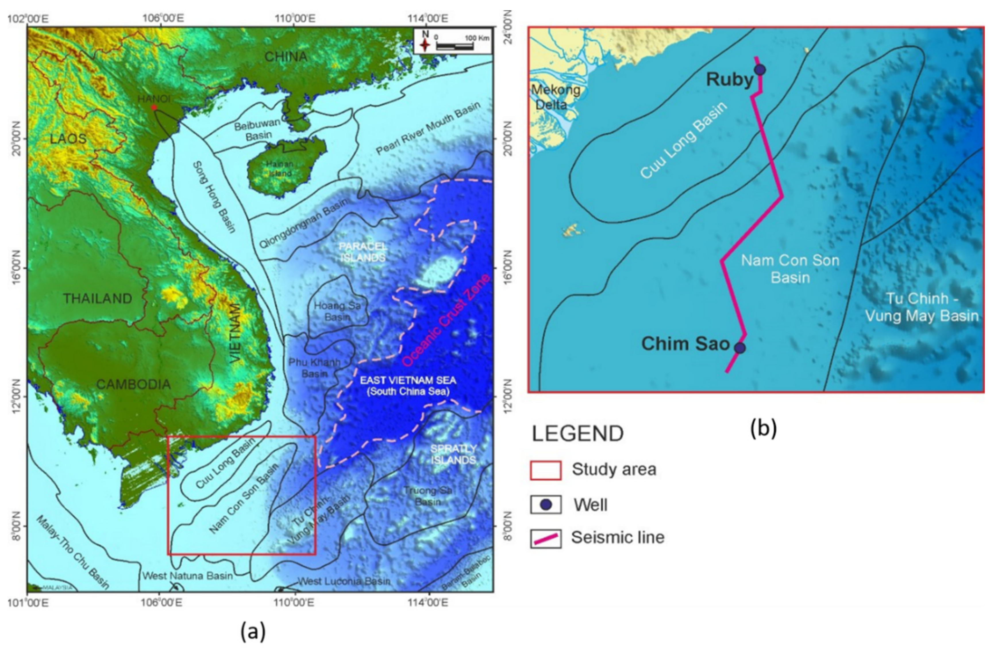
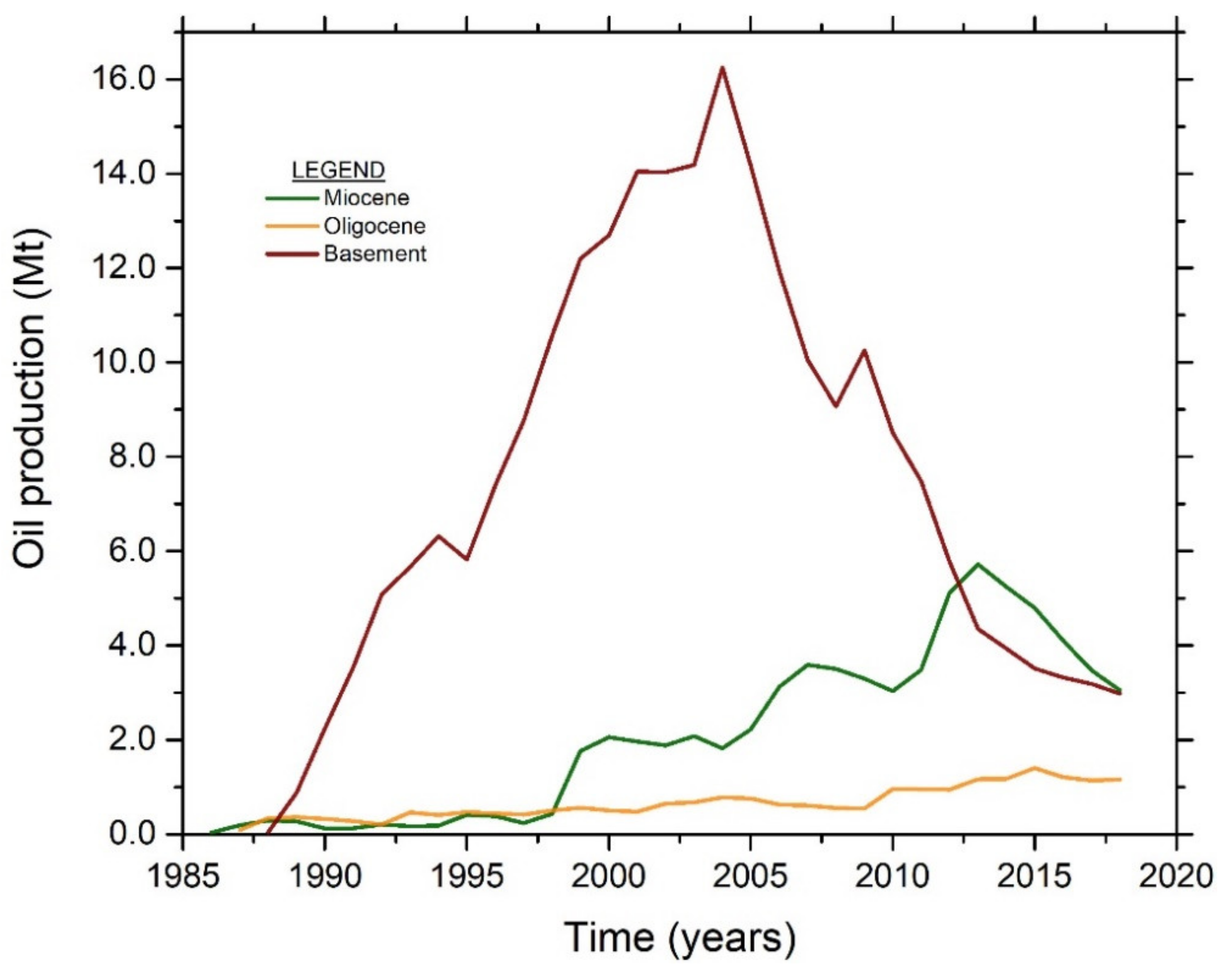
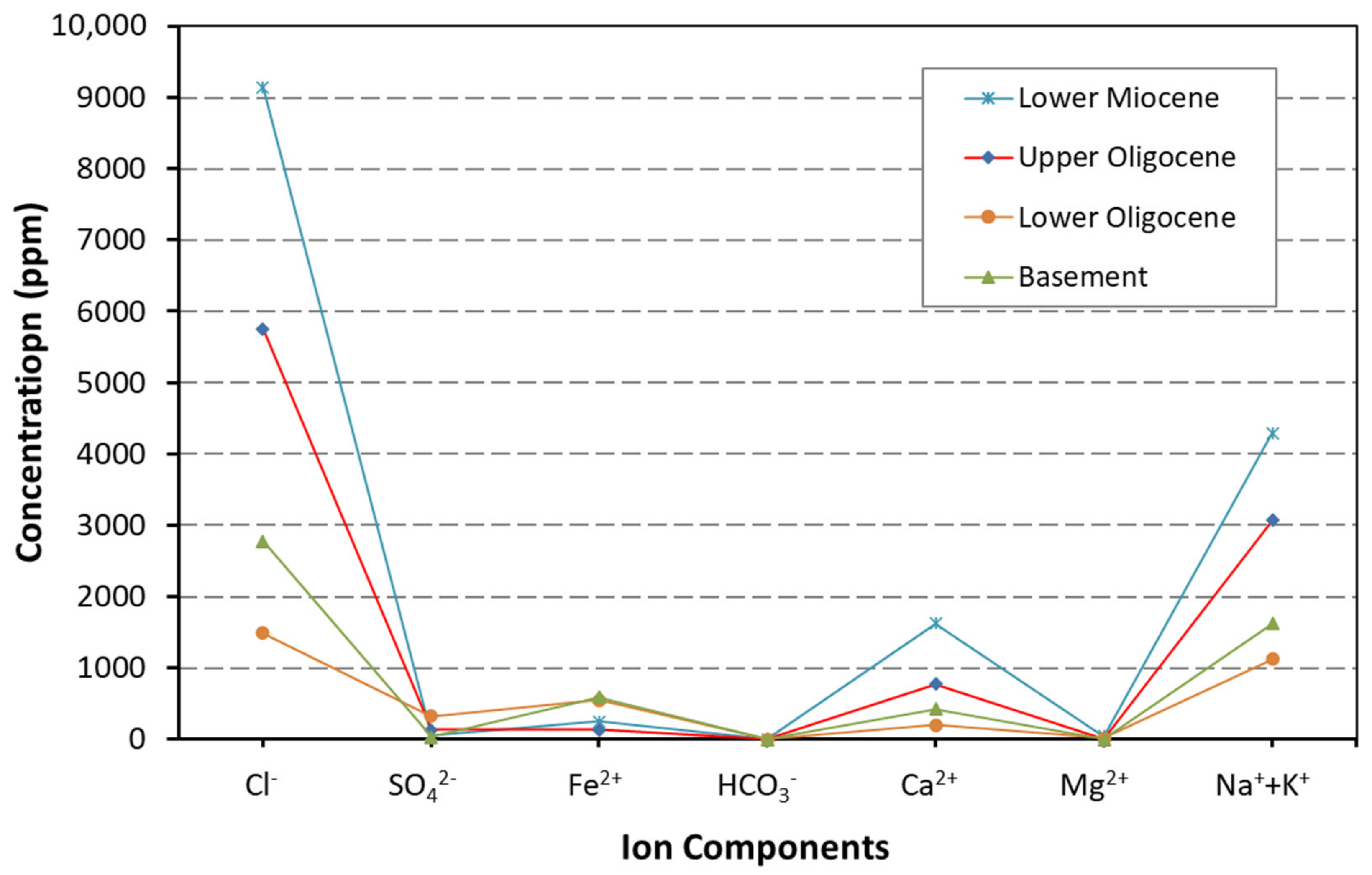
4.1. Geology of the Study Site

The Cuu Long Basin is separated from the Nam Con Son Basin to the SE by the Con Son Swell (Figure 11). The geologic history of the Cuu Long Basin can be divided into four phases as follows: (i) The pre-rift phase (Late Jurassic–Paleocene) with widespread emplacement of granitic plutons and NE-trending swarm dykes. These structural fabrics constitute the basis for the granitic basement play in the Cuu Long Basin; (ii) Rifting phase (Eocene ?–early Late Oligocene): in this period, the basin was opened in NW-SE direction, which reactivated earlier NE-SW trends as listric normal faults. These normal faults form grabens and half-grabens filled initially with coarse-grained sediments. As rifting continued and waned at the late Early Oligocene–early Late Oligocene, the basin expands into a widespread lacustrine environment; (iii) Compression phase (early Late Oligocene–early Early Miocene): Combined with pre-rift and syn-rift trends, the compression phases created pervasive fracture network in the granitic basement, which is crucial to the success of the basement play. Furthermore, during this time, lacustrine deposition is widespread and enabled the formation of the D shale, which is both an excellent source and seal for the basement play. Deep lake environment prevails throughout most of the D sequence and part of the C sequence; (iv) Thermal subsidence (late Early Miocene–Recent): After the compression phase, the basin entered a period of tectonic quiescence. The first major marine influence is marked by the Bach Ho shale (“Rotalid shale”), which can be correlated over the whole basin and serves as an excellent regional seal for the basin. Thermal subsidence and marine influence continued to the present day [45,46].

Figure 11 shows a long interbasin geological cross-section from the Cuu Long Basin, through the Con Son Swell, to the Nam Con Son Basin. The pre-Tertiary basement may be 6 to 8 km deep. The Ruby Field is located in the most northern part of Cuu Long Basin. The Ruby structure is an anticlinal drape that overlies one of these intra basin horst features. Hydrocarbon in the Ruby Field was discovered in the Early Miocene, Oligocene as well as the basement. The Nam Con Son Basin is separated from the Cuu Long Basin by a broad SW-NE trending basement ridge called Con Son Swell. It is about 550 km long and 200 km wide across its widest southern part. From the granitic outcrop on Con Son Island, it is believed that some part of Con Son Swell is built of Late Cretaceous granitoids. On the other hand, the Chim Sao Field is located towards the southwestern end of the Nam Con Son Basin. The stratigraphic section penetrated in the Chim Sao Field ranges in age from the recent strata to the Oligocene formation. Elsewhere in the Nam Con Son Basin, a basement of Late Jurassic to Early Cretaceous weathered and fractured granites and granodiorites have been penetrated. Hydrocarbon in Chim Sao Field was found in Early and Middle Miocene sands.

4.2. Results and Discussion

As the coreflooding experiment for LSWF is quite expensive and time-consuming in general, and for the Chim Sao field in particular, we have investigated the feasibility of LSWF using a numerical simulation approach in this study. First, the availability of low salinity water in this oil field is checked based on the reservoir petrophysical properties and production information. Figure 12 shows the ion concentrations of formation water of the main reservoir in the Chim Sao field, indicating that the Lower Oligocene formation water can be a good candidate for LSW source as its total salinity is essentially below 2000 ppm. In the first step of LSWF modeling for the Chim Sao field, the new code was applied to simulate a core flooding experiment with the input data of reservoir and fluid properties being shown in

Table 3. The petrophysical and physical properties of core samples collected from Chim Sao field, NCS Basin.

Description	Variables	Unit	HS Value (Lower Miocene Formation)	LS Value (Lower Oligocene Formation
Porosity	ϕ	%	14.7	14.7
Absolute permeability	K	mD	100	100
Reservoir temperature	T	°C	93	93
Corey water coefficient	nw	_	2.5	2
Corey oil coefficient	no	_	3.5	3
Water viscosity	μw	cP	0.45	0.42
Oil viscosity	μo	cP	3.55	n/c
Initial water saturation	sw,init	%	36.5	36.5
Connate water saturation	sw,c	%	20	20
Residual oil saturation	sor	%	20	15

. It is noted that the real ion concentrations of LSW from Lower Oligocene sand (the possible natural LSW source) and the formation water of the injected reservoir (Lower Miocene sand) were used in our LSWF simulation for the Chim Sao field. Figure 13 shows the results of simulated ion concentrations during the HS and LS injection stages, which show a very similar trend to those in Figure 10 for the Ruby field, where the injected water was an artificial one. Figure 14 shows the results of the recovery factor calculated for a two-stage LSWF simulation in the Chim Sao field, first with high salinity (HS) water flooding up to 4.4 PVI for maintaining reservoir pressure, then followed up by an LS water flooding up to 8 PVI. The simulation results obtained indicated that an EOR taking the natural LSW from Lower Oligocene to inject into the Lower Miocene oil sand could result in an increase of the recovery factor by 2.19%.

5. Conclusions and Recommendations

In this study, a comprehensive review of LSWF mechanisms was done. In line with a master EOR plan of PetroVietnam [7], the low salinity water flooding is considered as one of the possible EOR options to be applied for the mature and near-mature oil fields in Vietnam. To meet the need to quickly assess the LSWF feasibility of these oil fields, a new computation code using the finite element volume (FV) method was developed in Matlab to simulate a core flooding experiment, and it was successfully applied for the Chim Sao oil field in the Nam Con Son Basin. The major conclusions drawn from this study are as follows:

• Based on the results of a laboratory core flooding experiment conducted for the Ruby oil field in the Cuu Long Basin concerning a low salinity water flooding (LSWF) of the Lower Miocene sand, the multiple ion exchange (MIE) was identified by [8] as one of the most suitable mechanisms for this oil sand. The simulation conducted in this study also has confirmed the same for the Lower Miocene sand in the Nam Con Son Basin;
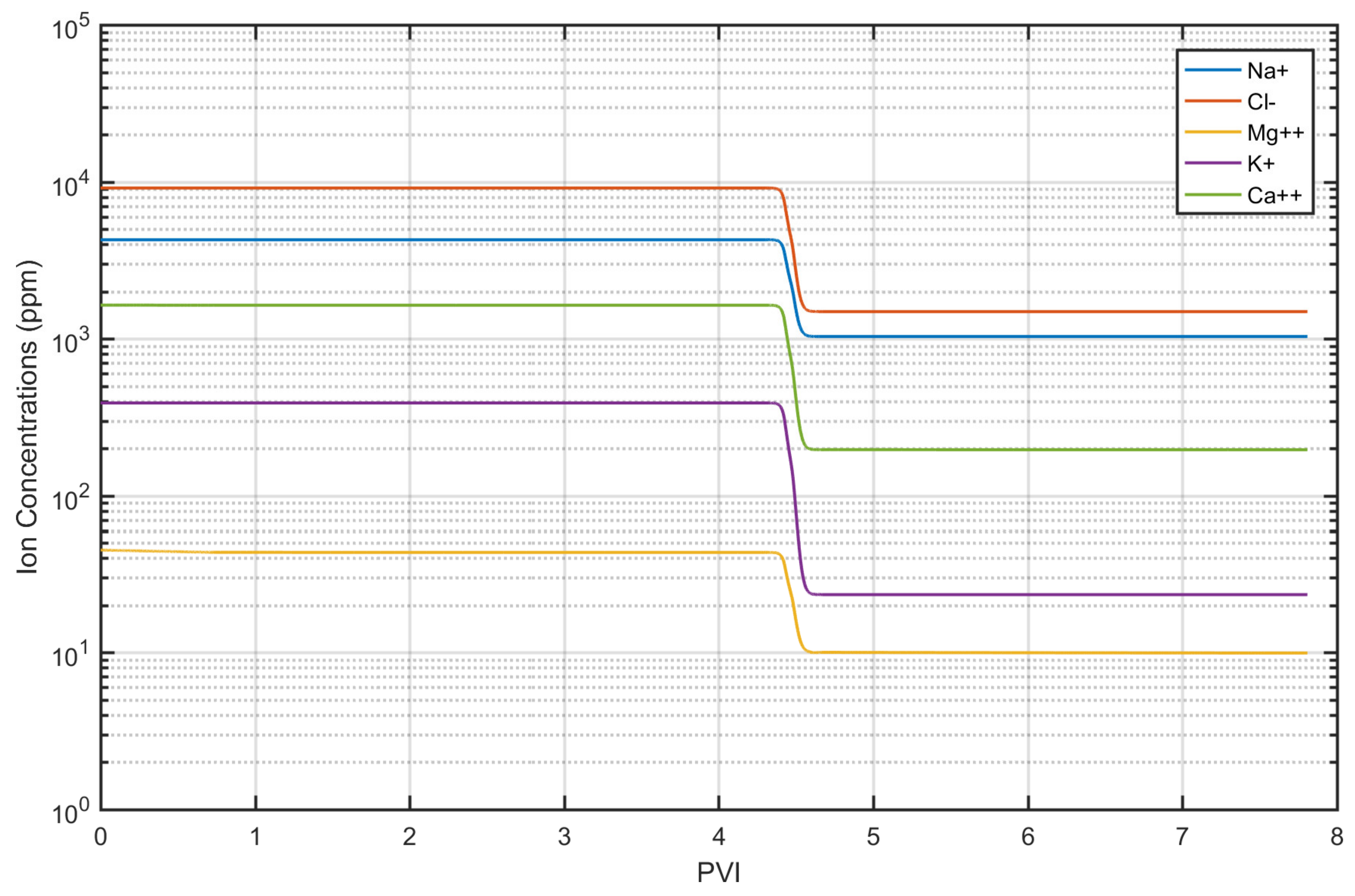
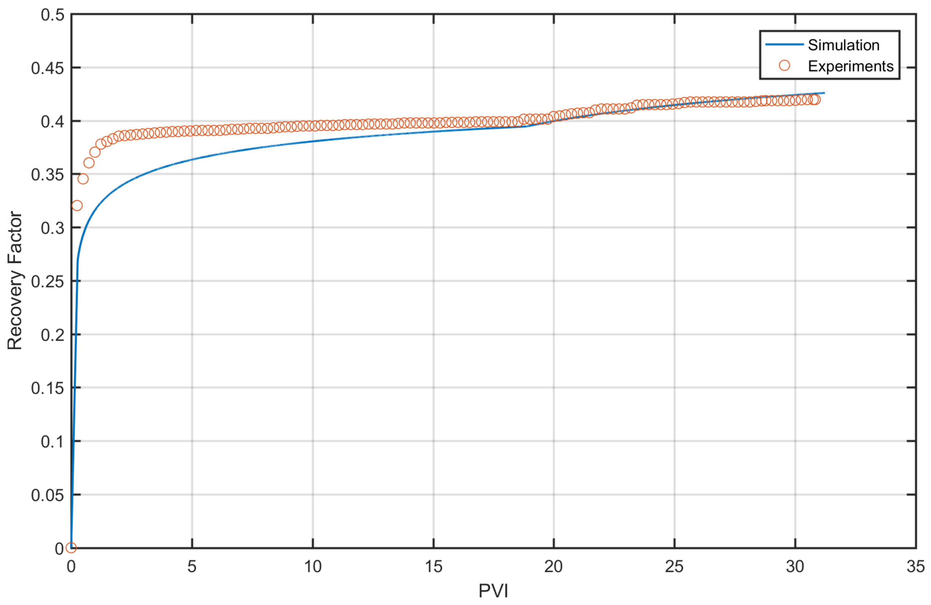
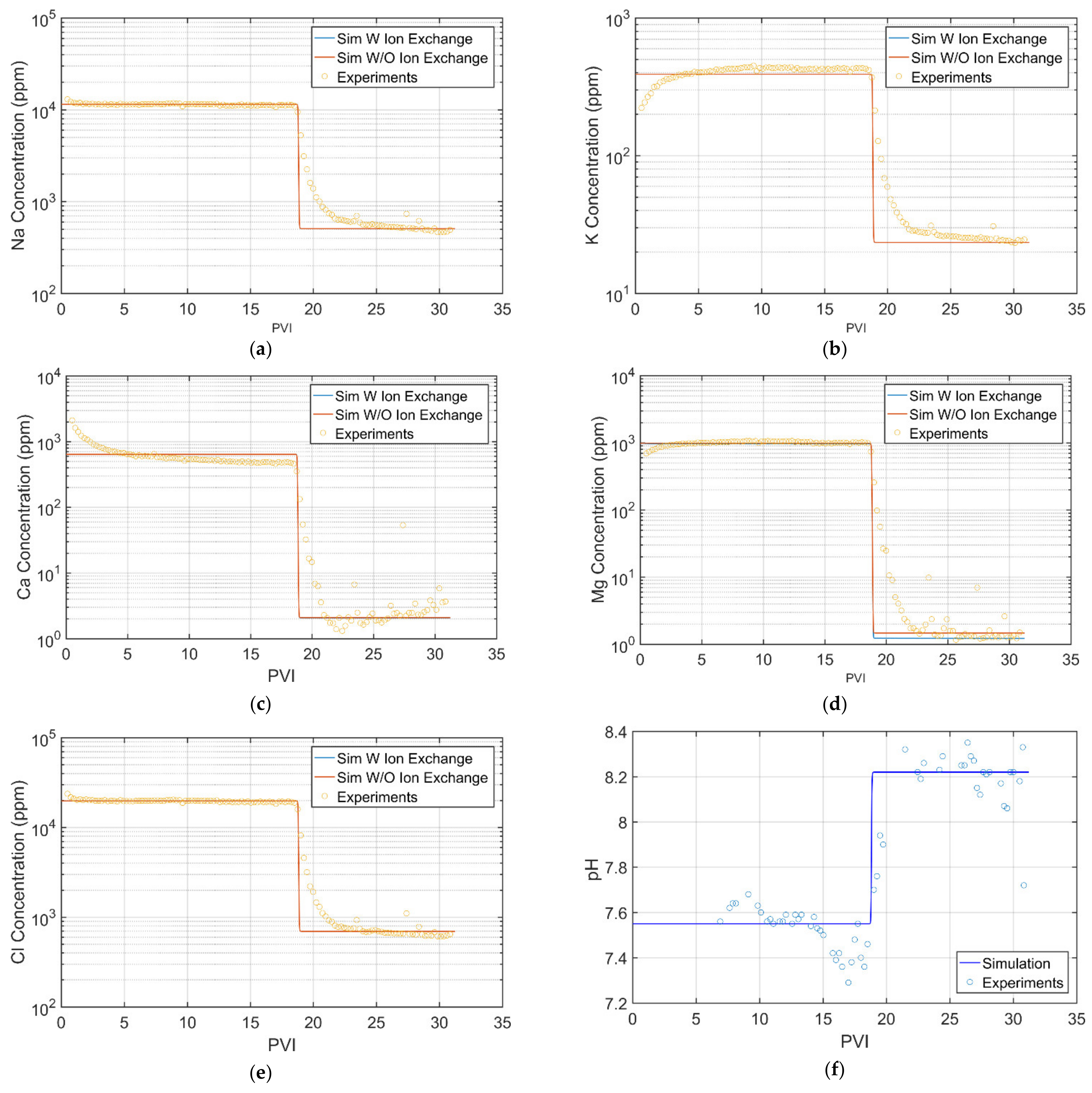
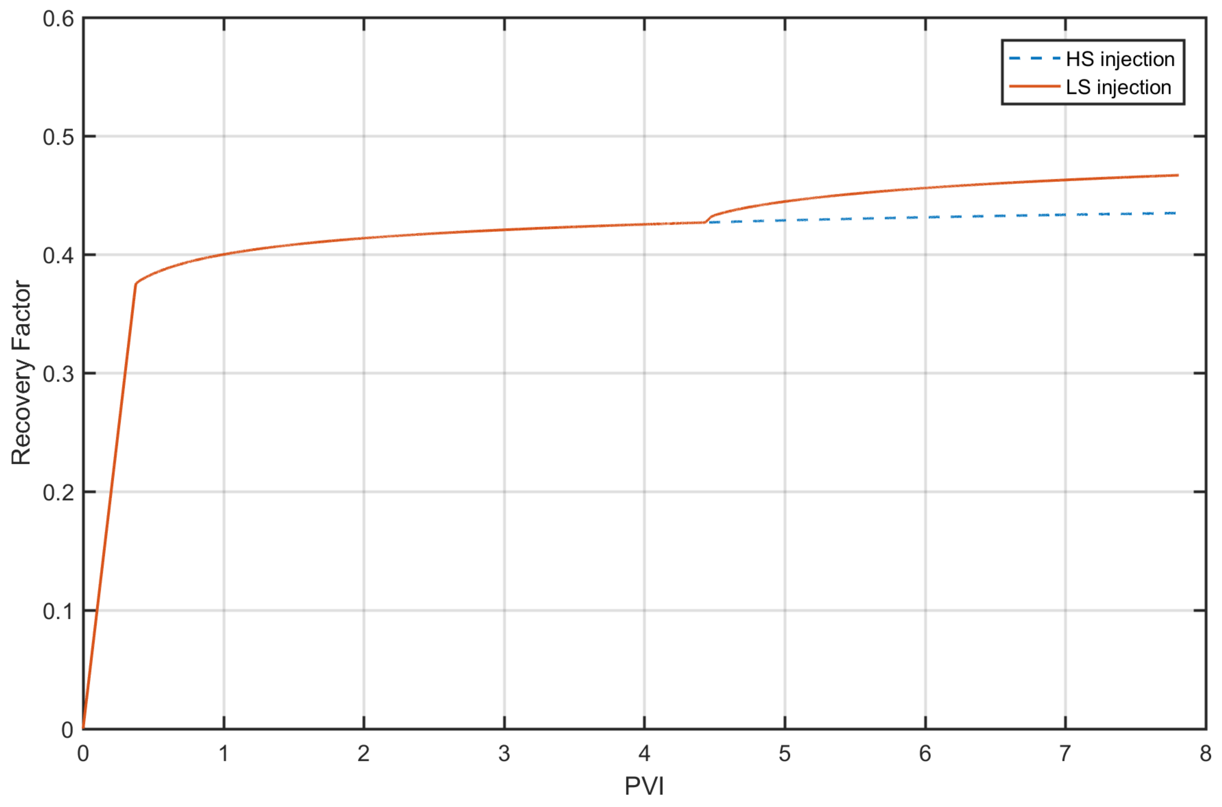
• A new computation code based on the finite volume element (FV) method was successfully developed in this study to simulate the ion transport in the aqueous in coupling with chemical reaction. The numerical simulations were run, and the results were compared with and are well-validated by the experimental results of the laboratory core flooding experiment for the Ruby field in the Cuu Long Basin in term of oil recovery factor, multi-ion concentrations (Na⁺, K⁺, Mg²⁺, Ca²⁺, Cl⁻ and H⁺);
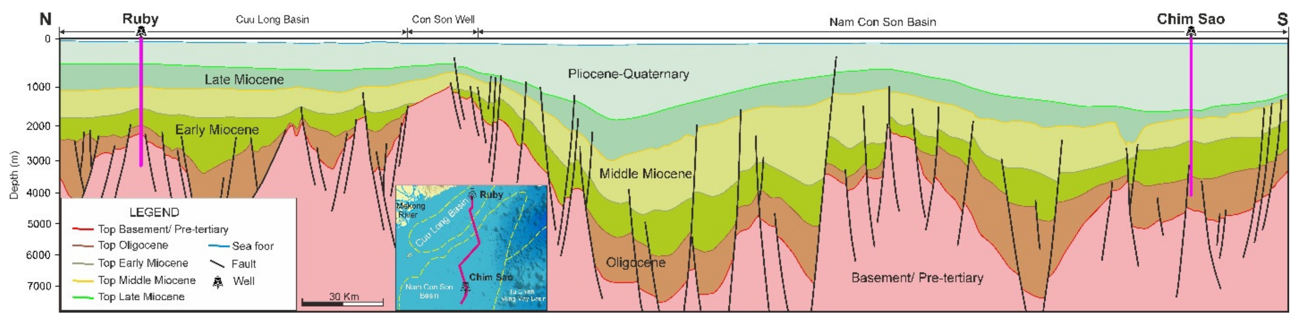
• This study’s major outcome was the successful simulation of LSWF using the natural low salinity water from the Lower Oligocene formation to inject into the overlying Lower Miocene sand, a main oil productive unit in the Chim Sao oilfield, the Nam Con Son Basin. The simulation results obtained show that such an LSWF could increase the oil recovery factor by 2.19%;
• It is recommended the application of the new code be applied for assessing the other mature oil fields in terms of applicability of LSWF to enhance their oil recovery, and some LSWF pilot full-scale field tests should be planned in the near future in the Nam Con Son Basin, Vietnam. In addition, further development of the code should consider the general form of flow equation (Equations (1a) and (1b)) in coupling with PhreeQC for chemical reactions the simulation to take care of the capillary pressure effect.

References

1. Thang, P.D.; Ngoc, P.Q.; Giao, P.H. A quick overview of oil matured field in Vietnam. In Proceedings of the SPE/VPI Virtual Workshop: Mature Field Development and IOR/EOR Technology, Hanoi, Vietnam, 23–25 February 2021. [Google Scholar]
2. Thang, P.D.; Giao, P.H. Polymer injection as a possible EOR method for a fractured granite basement reservoir in the Cuu Long Basin, Vietnam. J. Pet. Petrochem. Eng. 2017, 1, 129–140. [Google Scholar]
3. Thang, T.V. Application of Water-Alternating-Gas to Enhance Oil Recovery in the Miocene Reservoir, Cuu Long Basin; Hanoi University of Mining and Geology: Hanoi, Vietnam, 2020. [Google Scholar]
4. Thang, T.V.; Lan, L.X. Screening of water alternative gas injection method for enhanced oil recovery offshore viet nam oilfields. J. Mine. Tech. 2011, 34, 28–33. [Google Scholar]
5. Son, T.T.; Linh, H. Study on the Application of Thermal Stability Surfactant for High Temperature Reservoirs, Offshore Vietnam for Enhanced Oil Recovery; Vietnam Petroleum Insitute: Hanoi, Vietnam, 2011. [Google Scholar]
6. Linh, H.; Son, T.T.; Quy, N.M.; Long, H. Study on the Application of Nano—Surfactant for EOR of White Tiger Basement Reservoir, Offshore Vietnam; Vietnam Petroleum Institute: Hanoi, Vietnam, 2017. [Google Scholar]
7. Quy, N.M.; Long, H.; Giang, P.T. Enhanced Oil Recovery Master Plan for Mature Oil Fields, Offshore Viet Nam; Petro Vietnam: Hanoi, Vietnam, 2020. [Google Scholar]
8. Morishita, R.; Matsuyama, R.; Ishiwata, T.; Tsuchiya, Y.; Giang, P.T.; Takahashi, S. Oil and water interactions during low-salinity enhanced oil recovery in water-wet porous media. Energy Fuels 2020, 34, 5258–5266. [Google Scholar] [CrossRef]
9. Derjaguin, B.V.; Landau, L. Theory of the stability of strongly charged lyophobic sols and of the adhesion of strongly charged particles in solutions of electrolytes. Prog. Surf. Sci. 1993, 43, 30–59. [Google Scholar] [CrossRef]
10. Verwey, E.J.; Overbeek, T. Theory of the Stability of Lyophobic Colloids; Elsevier: New York, NY, USA, 1948. [Google Scholar]
11. McGuire, P.L.; Chatham, J.R.; Paskvan, F.K.; Sommer, D.M.; Carini, F.H. Low salinity oil recovery: An exciting new EOR opportunity for Alaska’s North Slope. In Proceedings of the SPE Western Regional Meeting, Irvine, CA, USA, 30 March–1 April 2005. [Google Scholar]
12. Austad, T.; RezaeiDoust, A.; Puntervold, T. Chemical mechanism of low salinity water flooding in sandstone reservoirs. In Proceedings of the SPE Improved Oil Recovery Symposium, Tulsa, OK, USA, 24–28 April 2010. [Google Scholar]
13. Tang, G.-Q.; Morrow, N.R. Influence of brine composition and fines migration on crude oil/brine/rock interactions and oil recovery. J. Pet. Sci. Eng. 1999, 24, 99–111. [Google Scholar] [CrossRef]
14. Sharma, M.M.; Filoco, P.R. Effect of brine salinity and crude-oil properties on oil recovery and residual saturations. J. Spe. 2000, 5, 293–300. [Google Scholar] [CrossRef]
15. Zhang, Y.; Morrow, N.R. Comparison of secondary and tertiary recovery with change in injection brine composition for crude-oil/sandstone combinations. In Proceedings of the SPE/DOE Symposium on Improved Oil Recovery, Tulsa, OK, USA, 22–26 April 2006. [Google Scholar]
16. Sheng, J.J. Critical review of low-salinity waterflooding. J. Pet. Sci. Eng. 2014, 120, 216–224. [Google Scholar] [CrossRef]
17. Nasralla, R.A.; Nasr-El-Din, H.A. Double-layer expansion: Is it a primary mechanism of improved oil recovery by low-salinity waterflooding. SPE Res. Eva. Eng. 2014, 17, 49–59. [Google Scholar] [CrossRef]
18. Anderson, W.G. Wettability literature survey-part 1: Rock/oil/brine interactions and the effects of core handling on wettability. J. Pet. Tech. 1986, 38, 1125–1144. [Google Scholar] [CrossRef]
19. Morrow, N. Wettability and its effect on oil recovery. J. Pet. Sci. Eng. 1990, 42, 1476–1484. [Google Scholar] [CrossRef]
20. Morrow, N.; Tang, G.; Valat, M.; Xie, X. Prospects of improved oil recovery related to wettability and brine composition. J. Pet. Sci. Eng. 1998, 20, 106–112. [Google Scholar] [CrossRef]
21. Srisuriyachai, F.; Pancharoen, M.; Laochamroonvoraponse, R.; Juckthong, P.; Kukiattikoon, A.; Sirirojrattana, B. Improvement of relative permeability and wetting condition of sandstone by low salinity waterflooding. In Proceedings of the IOP Conference Series: Earth and Environmental Science, Prague, Czech Republic, 2–4 July 2019. [Google Scholar]
22. Lager, A.a.W.K.J.; Black, C.J.J.; Singleton, M.; Sorbie, K.S. Low salinity oil recovery-an experimental investigation. Petrophysics 2008, 49, 28–35. [Google Scholar]
23. Rivet, S.M. Coreflooding Oil Displacements with Low Salinity Brine; University of Texas at Austin: Austin, TX, USA, 2009. [Google Scholar]
24. Fjelde, I.; Asen, S.M.; Omekeh, A.V. Low salinity water flooding experiments and interpretation by simulations. In Proceedings of the SPE Improved Oil Recovery Symposium, Tulsa, OK, USA, 14–18 April 2012. [Google Scholar]
25. Evje, S.; Hiorth, A. A model for interpretation of brine dependent spontaneous imbibition experiments. Adv. Water Resour. 2011, 34, 1627–1642. [Google Scholar] [CrossRef]
26. Hiorth, A.; Cathles, L.M.; Madland, M.V. The impact of pore water chemistry on carbonate surface charge and oil wettability. Transp. Porous Media 2010, 85, 1–21. [Google Scholar] [CrossRef]
27. Srisuriyachai, F.; Muchalintamolee, N. Cation interference in low salinity water injection in sandstone formation. In Proceedings of the 76th EAGE Conference and Exhibition, Amsterdam, The Netherlands, 16–19 June 2014. [Google Scholar]
28. Parkhurst, D.L.; Appelo, C.A.J. User’s Guide to PHREEQC (Version 2)—A Computer Program for Speciation, Batch-Reaction, One-Dimensional Transport, and Inverse Geochemical Calculations; Water-Resources Investigations Report; United States Geological Survey: Reston, VA, USA, 1999. [Google Scholar]
29. Lie, K. An Introduction to Reservoir Simulation Using Matlab/GNU Octave: User guide for the MATLAB Reservoir Simulation Toolbox (MRST); Cambridge University Press: Cambrige, UK, 2019. [Google Scholar]
30. Bao, K.; Lie, K.; Møyner, O.; Liu, M. Fully implicit simulation of polymer flooding with MRST. J. Comput. Geosci. 2017, 21, 1219–1244. [Google Scholar] [CrossRef]
31. Mykkeltvedt, T.S.; Raynaud, X.; Lie, K.-A. Fully implicit higher-order schemes applied to polymer flooding. J. Comput. Geosci. 2017, 21, 1245–1266. [Google Scholar] [CrossRef]
32. Shojaei, M.; Ghazanfari, M.H.; Masihi, M. Relative permeability and capillary pressure curves for low salinity. J. Nat. Gas. Sci. Eng. 2015, 25, 30–38. [Google Scholar] [CrossRef]
33. Koenig, H. Modern Computational Methods. In Series in Computational and Physical Processes in Mechanics and Thermal Sciences; Taylor & Francis: Oxfordshire, UK, 1998. [Google Scholar]
34. Pozrikidis, C. Fluid Dynamics: Theory, Computation, and Numerical Simulation; Springer: New York, NY, USA, 2009. [Google Scholar]
35. Alsofi, A.M.; Blunt, M.J. Control of Numerical Dispersion in Simulations of Augmented Waterflooding. In Proceedings of the SPE Improved Oil Recovery Symposium, Tulsa, OK, USA, 24–28 April 2010. [Google Scholar]
36. Jerauld, G.R.; Webb, K.J.; Lin, C.-Y.; Seccombe, J. Modeling low-salinity waterflooding. In Proceedings of the SPE Annual Technical Conference and Exhibition, San Antonio, TX, USA, 24–27 September 2006. [Google Scholar]
37. Jerauld, G.R.; Lin, C.; Webb, K. Modeling low salinity waterflooding. Spe. Res. Eval. Eng. 2008, 11, 1000–1012. [Google Scholar] [CrossRef]
38. Lantz, R.B. Quantitative evaluation of numerical diffusion (truncation error). J. Soci. Pet. 1977, 11, 315–320. [Google Scholar] [CrossRef]
39. Wouter, J.D. Simulation of Geochemical Processes during Low Salinity Water Flooding by Coupling Multiphase Buckley-Leverett Flow to the Geochemical Package PHREEQC—A Case Study for an Oil Field on the Norwegian Continental Shelf; University of Technology Delft: Delft, The Netherlands, 2012. [Google Scholar]
40. Hirsch, C. Numerical Computation of Internal and External Flows—Fundamentals of Computational Fluid Dynamics; Elsevier: Oxford, UK, 2007. [Google Scholar]
41. Chen, Z. Reservoir Simulation: Mathematical Techniques in Oil Recovery; Society for Industrial and Applied Mathematics (SIAM): Philadelphia, PA, USA, 2008. [Google Scholar]
42. Charlton, R.S.; Parkhurst, D.L. Modules based on the geochemical model PHREEQC for use in scripting and programming languages. Comput. Geosci. 2011, 37, 1653–1663. [Google Scholar] [CrossRef]
43. Corey, A. The interrelation between gas and oil relative permeabilities. Prod. Mon. 1954, 19, 38–41. [Google Scholar]
44. Tripathi, I.; Mohanty, K. Instability due to wettability alteration in displacements through porous media. J. Chem. Eng. Sci. 2015, 63, 5366–5373. [Google Scholar] [CrossRef]
45. Huchon, P.; Nguyen, T.N.H.; Chamot-Rooke, N. Finite extension across the South Vietnam basins from 3D gravimetric modelling: Relation to South China Sea kinematics. Mar. Pet. Geol. 1998, 15, 619–634. [Google Scholar] [CrossRef]
46. Tapponnier, P.; Peltzer, V.; Armijo, R. On the mechanics of the collision between India and Asia. Geol. Soc. Lond. Spec. Publ. 1986, 19, 113–157. [Google Scholar] [CrossRef]
Figure 1. Oil production profiles of Lower Miocene clastic reservoirs of Cuu Long Basin.
Energies 14 02658 g001
Figure 2. Low-salinity water flooding (LSWF) as one applicable method in the enhanced oil recovery (EOR) master plan of Petro Vietnam after Quy et al. 2020 [7].
Energies 14 02658 g002
Figure 3. The petroleum basins in Vietnam (a) and the study location in the Nam Con Son Basin (b).
Energies 14 02658 g003
Figure 4. Low salinity mechanisms of multiple ions exchange (MIE) with potassium replacing calcium and liberation of oil in the form of calcium carboxylate complex, modified after [27].
Energies 14 02658 g004
Figure 5. Finite volume (FV) discretization for simulation of 1D core flooding by Low Salinity Water (LSW) using N + 1 grid cells.
Energies 14 02658 g005
Figure 6. Workflow of LSWF numerical solutions by coupling chemical components transport and IPhreeQC.
Energies 14 02658 g006
Figure 7. Core flooding experiment apparatus for LSW [8].
Energies 14 02658 g007
Figure 8. Relative permeability.
Energies 14 02658 g008
Figure 9. Comparison of the recovery factor of LSWF simulation and experiment for the Ruby field core.
Energies 14 02658 g009
Figure 10. Results of LSWF simulation versus the experimental ones for the Ruby field. (a)–(d)the simulated and experimental concentrations of Na, K, Ca and Mg; (e)the simulated and experimental concentration of passive ion; (f) an increasing trend of pH.
Energies 14 02658 g010
Figure 11. An interbasin geological cross-section showing the Ruby field in the Cuu Long Basin and the Chim Sao field in the Nam Con Son Basin.
Energies 14 02658 g011
Figure 12. Formation water of the main reservoir in the NCS Basin.
Energies 14 02658 g012
Figure 13. The ion concentrations calculated by the new code during a two-stage water flooding simulation for the Chim Sao field core sample.
Energies 14 02658 g013
Figure 14. Recovery factor calculated during a two-stage water flooding of high salinity (HS) to 4.4 Pore Volume Injection (PVI) and Low Salinity (LS) from 4.4 to 8 PVI for the Chim Sao core sample.
Energies 14 02658 g014