Abstract
The power quality of the Electrical Power System (EPS) is greatly affected by electrical harmonics. Hence, accurate and proper estimation of electrical harmonics is essential to design appropriate filters for mitigation of harmonics and their associated effects on the power quality of EPS. This paper presents a novel statistical (Least Square) and meta-heuristic (Grey wolf optimizer) based hybrid technique for accurate detection and estimation of electrical harmonics with minimum computational time. The non-linear part (phase and frequency) of harmonics is estimated using GWO, while the linear part (amplitude) is estimated using the LS method. Furthermore, harmonics having transients are also estimated using proposed harmonic estimators. The effectiveness of the proposed harmonic estimator is evaluated using various case studies. Comparing the proposed approach with other harmonic estimation techniques demonstrates that it has a minimum mean square error with less complexity and better computational efficiency.
1. Introduction
Recently, estimation and mitigation of electrical harmonics have attained much attention due to excessive integration of non-linear, power electronic components and renewable energy sources in an Electrical Power System (EPS) [1,2]. Harmonics can be described as distortion in the fundamental voltage/current waveform of the electrical signal. In an EPS, a higher value of Total Harmonic Distortion (THD) can cause various drawbacks like deterioration of electrical components, increased power loss, and interferences for communication systems. The power quality of EPS is directly influenced by electrical harmonics. Hence, it is necessary to properly estimate and mitigate the electrical harmonics for smooth and stable operation of EPS. Moreover, various regulations and standards have been developed for harmonic levels by authorized organizations like the International Electrotechnical Commission (IEC) and Institute of Electrical and Electronics Engineers (IEEE) [3,4].
So far, various studies have been performed to model, eliminate, measure, and estimate electrical harmonics to mitigate their adverse effects. The essential problem among mentioned studies is the estimation of electrical harmonics, and different methodologies were proposed in literature to solve this issue. The accurate approximation of electrical harmonics in EPS is an extremely complex and multimodal problem [5]. Moreover, electrical harmonics are getting more prominent due to the continuous integration of non-linear power electronics equipment. Time varying noisy environment makes this problem even more complex and dynamic. So, the solution to the harmonic estimation (HE) problem needs to be upgraded [6,7]. The harmonic estimation problem deals with two types of approximations. The first one is the detection of harmonics amplitude and the second one is the detection of the harmonics phase. Amplitude estimation of particular harmonics is a linear problem, while phase and frequency estimation of particular harmonics is a nonlinear problem [8,9]. Frequency estimation of power system harmonics and their transient analysis are also sometimes resolved in harmonic estimation problem [4,10,11].
In literature, researchers solved HE problem via various mathematical, statistical, and heuristic methodologies stated in Figure 1. Initially, mathematical techniques like Fourier transform, fast Fourier transform, and discrete Fourier transform are applied, but their disadvantages, like spectral leakage, picket fence, and those which were only applicable for static signals, lead the researchers to explore more efficient tools for HE problem [12,13,14]. Partial accuracy was achieved by applying Hilbert and wavelet transformation [11,15]. To achieve greater accuracy, artificial intelligence techniques like Fuzzy Logic, Neural Network, Expert systems, and ADALINE are also used [16,17]. Although they had accurate results but their computational efficiency is very low.
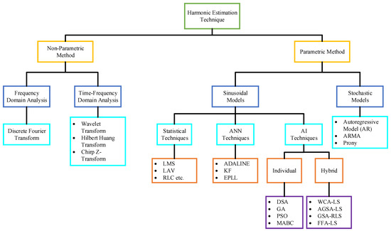
Figure 1.
Classification of methodologies used for HE problem.
To enhance computational efficiency, several statistical techniques like Kalman filter (KF), Least square (LS), Least mean square (LMS), Recursive least square (RLS), and Least average value (LAV) were adopted to solve HE problem [18,19,20,21,22]. These techniques had a simple structure, linear behavior, and higher efficiency than mathematical and AI techniques. However, their flaws, like requirement of system information and fine-tuning of the system make them difficult to be utilized.
Recently, hybrid statistical and nature inspired meta-heuristic techniques have acquired huge attention of researchers due to their self-adaptive nature, less computational efficiency, smooth structure, and solving complex engineering problems. Different strategies were reported in literature for addressing HE problem, i.e., Local Ensemble Kalman filter (LETKF) [23,24], Kalman filter and least error square (KFLES) [25], Phase-locked loop (PLL) [24,26], Particle swarm-Passive congregation (PSOPC) [27,28], Genetic Algorithm (GA) [29], Bacterial Foraging-Recursive (BFO-RLS) [30,31], Bacterial Swarming [32], Firefly algorithm (FFALS) [33], Artificial bee (ABCLS) [34], Biogeography-RLS [35], Differential search [36], Gravity search-RLS [37], A modified ABC (MABC) [3], and Frequency shifting-filtering method (FSF) [38]. GWO equipped with evolutionary operators [39] is also implemented for HE problems but it has large computational time due to the addition of tournament, selection, crossover, and mutation operators. Although the accuracy and computational efficiency of the aforementioned techniques are better but they offer complex structures with large controlling parameters. Moreover, above-mentioned studies have not estimated the frequency component of the signals, and the effectiveness of proposed estimators have been validated only on steady state conditions. However, few studies in the literature estimate the frequency component of the electrical signals [40,41], but they have not included transient conditions to authenticate the performance of HE estimator. While there is a dearth of studies [4,10,11] that considered transient conditions in HE problem, the methodologies utilized in the referred studies are based on statistical techniques that provide better accuracy, but their computational efficiency is very low. The accurate estimation of harmonics in an electrical signal (both in steady and transient state) can be further improved with the latest advancements in solution tools.
From the literature survey, it could be observed that each methodology implemented on the HE problem has its own pros and cons. Some techniques had optimal results but poor computational efficiency and some provide great computational efficiency but compromise accuracy. The authenticity of the literature harmonic estimators in the dynamic and composite power system, tends to be lessening. The investigators are advancing towards an updated estimator that can perform well in both steady and transient conditions with less complexity level, more accuracy, and low computational efficiency. So, it still needs a proper solution that can tackle the HE problem with better accuracy, having less computational time than the state-of-the-art techniques. The major contribution of this paper is as follows:
- A novel Grey Wolf Optimizer (GWO) and LS-based hybrid estimator is proposed for accurate estimation of harmonics in EPS.
- The proposed GWO-LS has the ability to cope with HE problems timely in the modern dynamic and complex smart grid/system.
- GWO is utilized for accurate estimation of non-linear part, and LS is used for accurate estimation of the linear part of HE problems.
- GWO is also utilized for the accurate estimation of frequency components of integral, sub, and inter harmonics.
- The transient analysis of the case studies is done to ascertain the effectiveness of the proposed GWO-LS harmonic estimator.
- The proposed harmonic estimator performed better in dynamic and noisy signals, reduces complexity level, and improves the presented harmonic estimator’s computational efficiency and accuracy.
- The effectiveness of the proposed estimator is evaluated on standard test systems used by various researchers.
2. Problem Formulation of Harmonic Estimation
The estimation of electrical voltage or current signals having electrical harmonics of dynamic nature is computed in two stages. The first stage deals with the non-linear approximation of harmonic’s phase and frequency by GWO, while the second stage deals with the harmonic’s amplitude approximation. Generally, an electrical signal containing harmonics is represented by the summation of sine-cosine functions having higher frequencies values that are integral multiples of the fundamental frequency and is given as [3],
where represents harmonic order, shows harmonic amplitude, indicates angular frequency while states harmonic’s phase. DC offset is shown by and is given as,
The entire model of a signal having noise is given by [37]:
here, stands for total noise in a specific signal. The digital representation of the above signal is represented as:
where shows sample number and represents sampling time. Applying trigonometric identity on the above equation yields:
Expanding decaying offset and neglecting higher frequency terms update the above equation as,
The equation to be estimated for the estimated signal becomes:
where and is the matrix of known and unknown parameters, respectively, while is updated successfully to approximate signal . The amplitude and phase of an unknown th harmonic with the decaying dc component after the matrix is updated can be as:
Finally, the objective function for the harmonic estimation problem is formulated as [6]:
here, is our actual power signal while is the final approximated signal by GWO-LS.
3. Proposed Methodology
3.1. Grey Wolf Optimizer
GWO is a nature inspired-heuristic algorithm proposed by Seyed Ali Mirjalili [42] and is widely employed to obtain the optimal solution for various optimization problems. GWO is inspired by the social behavior of grey wolves; naturally, they live in a group form called packs, and the members of each group vary from 5 to 12. Strong social hierarchy is a unique feature of grey wolves. This social hierarchy is based on four ranks of wolves that are termed as alpha (α), beta (β), delta (δ), and omega (ω) wolf. The ‘α’ is the superior of all because of its leadership quality, managerial skills, and decision-making power, while ‘β’ wolf is inferior to α and acts as its adviser but discipliner for the rest of the pack. The third level belongs to delta wolves, and they submit themselves to both alpha and beta wolves. They are also helpful in hunting, care-taking of the whole pack. The lowest level of the pack is an omega wolf having lethargic nature.
Another fascinating phenomenon of grey wolves is their unique hunting mechanism, which undergoes five steps: (1) tracking, (2) chasing, (3) encircling, (4) harassing, and (5) attacking. Figure 2 displays the complete hunting process of grey wolves. Figure 2A shows the wolf tracking and chasing, while Figure 2B–D reveals how wolves encircle and harass their prey. Similarly, the attacking behavior of wolves is depicted in Figure 2E. The encircling behavior of the grey wolf is modeled using the following equations.
where presents the current iteration, shows the distance between specific wolf and prey while and are the control variables for updating iteration. indicates the best location of grey wolves (Local best) while depicts the position of prey with respect to the grey wolf (Global best). The coefficient vectors and are computed as follows:
where is computed using and its value decreases from 2 to 0. is a control variable having a value in the range of 0–2 while and are two random numbers between [0, 1]. The hunting mechanism of the grey wolf is modeled by:
here, and represent the position of from the prey and distance between and prey, respectively. Similarly, , , , and describe the position and distance of respective wolves. The grey wolves terminate the hunting step by attacking the prey, and the attacking phenomenon relates to the exploitation phase of the GWO algorithm. The value of decreases from 2 to 0 to model the attacking behavior. The position vector is a random value in the range of [−2, 2]. When the value of variable lies in [−1, 1], the new position of the searching agent can be generated at any point between its current location and the prey location. If || < 1 (convergence), this value compels the wolf for attacking the prey, while if || > 1 (divergence) wolves search more for the better prey (exploration process) as shown in Figure 3. Another coefficient vector supports the searching mechanism of GWO, and it describes the obstacles which can occur in nature during the hunting step. The value of allows the wolf to prevent obstacles and approach the prey. Therefore, we can say that and are the control variables here.
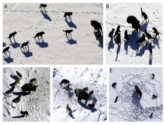
Figure 2.
Prey Hunting mechanism of Grey Wolves [42]. (A) tracking and chasing (B–D) encircling and harassing and (E) attacking.
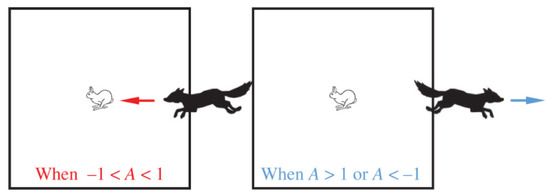
Figure 3.
Exploration and Exploitation in GWO.
3.2. Hybrid GWO-LS Harmonic Estimator
In this paper, a hybrid of statistical technique Least square method (LSM) [43] and a meta-heuristic technique GWO is proposed to solve the HE problem. The purpose of hybridizing two different nature techniques is to minimize the computational burden, increasing computational efficiency and accurate estimation of harmonics. The prominent feature of GWO is its social hierarchy and is well adapted for solving complex problems, and its working methodology is explained in the previous section, while the selection of LSM to develop the proposed harmonic estimator is based on various reasons. Firstly, it reduces the computational time of the GWO. Secondly, it moves to an exact solution as a statistical technique rather than trapping in local optima. So, it provides accurate results in linear estimation (Estimation of harmonic amplitude) of the HE problem. Thirdly it reduces the computational burden of the GWO and improves the convergence characteristics of GWO-LS as a whole. In the proposed hybrid harmonic estimator, LSM is utilized for accurate estimation of the linear part (harmonic amplitude) of the HE problem, while GWO is utilized for a proper approximation of the non-linear part (harmonic phase and frequency) of the HE problem.
For proper estimation of harmonics in the desired signal, which is a matrix of grey wolves having number of searching agents are initialized according to a number of power system harmonics to be estimated. The objective function of the HE problem is to minimize Mean Square Error (MSE). First of all, a matrix of number of searching agents (Grey Wolves) is defined where the location of a single searching agent consists of number of harmonics.
Numerous searching agents combine to form an agent matrix .
here, indicates the population size of grey wolves, and is the total harmonics number in a single search agent. A single searching agent consists of various locations, and these locations are equal to the total number of harmonics in a signal. The location of each search agent is initialized randomly as follows:
where and are the lower and upper bounds specified by the HE problem, respectively. The GWO-LS estimator aims to properly approximate the harmonics’ amplitude and phase of the harmonics in a time-varying noisy environment.
The error signal, which is obtained by the comparison of the actual signal and approximated signal, is fed to the optimization framework. This framework operates to derogate the estimation error until best result is obtained. The proposed harmonic estimator GWO-LS is said to be the least complex estimator due to the smaller number of control variables. It has only two control variables irrespective of GA-LS having four, PSO-LS having five, BFO having four, F-BFO-LS having six, BFO-RLS having four, BBO-RLS having four, GSA-RLS having five, and MABC having four controlling variables that improve the computational time ultimately. The detail description of GWO-LS tuning parameters is given in Table 1 while the detailed flowchart of GWO-LS is depicted in Figure 4.

Table 1.
Tuning Parameters for GWO-LS framework.
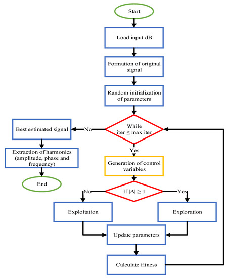
Figure 4.
Flowchart of GWO-LS Harmonic Estimator.
3.3. Computational Procedure
The proposed methodology to solve the HE problem comprises of following steps:
- Load input database.
- A signal named “original signal” is formulated by utilizing an input database.
- Initialization of HE and GWO-LS parameters.
- GWO-LS is applied for updating unknown parameters.
- Formation of estimated signal by updated parameters.
- Comparison of the original signal and estimated signal to evaluate objective function (MSE).
4. Simulation Results and Discussion
In this paper, two case studies are utilized to validate the effectiveness of the proposed harmonic estimator. These case studies are widely used in literature for the comparative analysis of the HE problem and are given as:
- Test System I: Estimating integral harmonics without including Sub and Inter harmonics in time-varying noisy environments.
- Test System II: Estimation of integral harmonics including Sub and Inter harmonics in a time-varying noisy environment.
The signal-to-noise ratio levels are selected as 10 dB, 20 dB, and 40 dB for a fair comparison of the proposed estimator with literature available estimators. In addition to creating time varying noisy environment, the constructed signals are made more complex for estimation by including transients at different time intervals. Moreover, three different performance indicators are utilized to examine the performance of the proposed GWO-LS estimator in comparison with the state-of-the-art estimator available in the literature. The selected performance indicators are given as:
- Mean Square Error (MSE) which can be computed using (13).
- Residual Sum of Squares (RSS) and is calculated as:
- Performance Index (PER) is another evaluation indicator used in this study for the comparison of GWO-LS with the state of art techniques and is determined as:
The simulation work is carried out in MATLAB 2019a programming environment on a personal computer having Windows 8 operating system with a 2.30 GHz processor and 6GB RAM.
4.1. Test System I: Estimation of Integral Harmonics without Including Sub and Inter Harmonics in Time-Varying Noisy Environment
The test signals generated by variable frequency drives (VFDs), electric arc furnaces, and power electronics devices are used for the estimation of integral harmonics in the current study. These signals are extensively used in literature for the comparative analysis of various harmonic estimators. The data of frequency, phase, and amplitude required for these signals is given in Table 2. The original test signal, which is a continuous signal, is generated using data provided in Table 1 [3,39]. The test signal is modeled and discretized by a renowned Nyquist criterion having 64 samples in one cycle, and the sampling frequency is set to be 3.2 kHz. The GWO-LS framework has been applied to estimate harmonics in this test signal having multiple levels of adaptive noise with the inclusion of decaying DC offset. The time-varying noisy environment is created by adding the different random noises and DC offset values in the original signal. To validate the performance of presented estimator in approximating dynamic parameters, a short transient is produced in 5th harmonic from 0.12 s to 0.26 s.
Table 2.
Harmonic Contents of Actual Signal.
The simulation parameters for the HE problem and GWO-LS are stated in Table 3. These values are taken from the literature harmonic estimators [3,39,43]. Moreover, the parametric values of Table 3 are selected in such a way so that a fair comparison between the proposed and literature harmonic estimator can be performed. The searching agent is an important simulation parameter. Its value is selected as 50 because the MSE comes out to be least for this value. The variation of Evaluation parameters with respect to searching agents is shown in Figure 5.
Table 3.
Case Study I Parameters for Simulation.
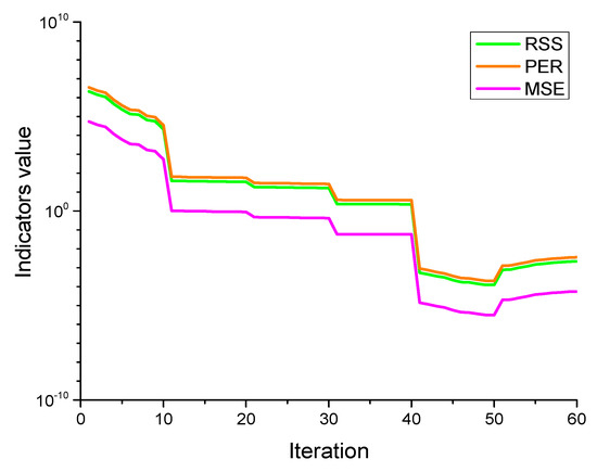
Figure 5.
Variation of evaluation parameters of RSS, PER and MSE with respect to searching agents.
Two signals are generated using the proposed harmonic estimator; the first one is the actual original signal made from input data with five integral harmonics. The second signal is an approximated one that is obtained by GWO-LS containing the approximated harmonics amplitudes and phases. These two signals are compared via MSE. The actual and approximated harmonics are then compared with respect to the percentage error. The simulation is carried out on four signals which are actual signals with no noise, a signal having 40 dB, 20 dB, and 10 dB noises (SNRs). The output values of best and worst harmonics amplitudes and phases with their percentage errors from actual harmonic values are tabulated in Table 4.
Table 4.
Case Study I Parameters after Simulation.
The comparison of actual and estimated signals is shown in Figure 6 at different SNRs. It is evident from Figure 6a that the estimated signal using GWO-LS exactly matches the original signal. However, it can be observed from Figure 6c,d that the signals become corrupted with the addition of different noise levels and decaying DC offset. In the presence of a 40 dB noise level, the proposed GWO-LS estimator accurately approximates the original signal while small deviations are observed in the original and the approximated signal when added noise is 20 dB. The estimation of the signal is more difficult in the presence of a 10 dB noise level, but a comparison of results from Table 5 indicates that the GWO-LS estimator outclasses the state of art techniques in such complex signal estimation.
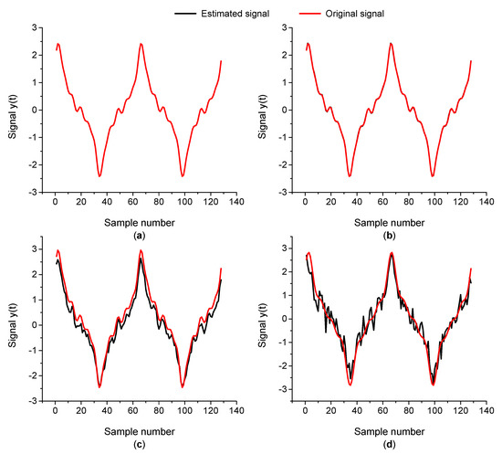
Figure 6.
Actual and Estimated signal comparison (a) non-noisy, (b) 40 dB noise level, (c) 20 dB noise level, and (d) 10 dB noise level.
Table 5.
GWO-LS Numerical Comparison for Case Study I.
The convergence characteristics of the proposed GWO-LS estimator using selected indicators at different noisy signals are shown in Figure 7. The proposed estimator converges in less than 120 iterations for a non-noisy signal estimation. Similarly, GWO-LS takes 145, 162, and 184 iterations to converge for the 40 dB, 20 dB and 10 dB signal, respectively. Figure 7 indicates that the number of iterations to converge increases as the signal’s noise level increases. It is evident from this Figure that the proposed harmonic estimator takes a higher time for the convergence of signal having a higher noise level. The computational time comparison of GWO-LS with the literature techniques is given in Table 6. It can be observed that the computational efficiency of the proposed harmonic estimator is much higher.
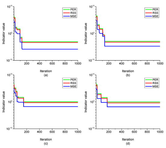
Figure 7.
The convergence characteristics of the GWO-LS framework for the case study I (a) non-noisy signal (b) 40 dB (c) 20 dB and (d) 10 dB.
Table 6.
GWO-LS Numerical Comparison for Case Study II.
The convergence behavior of GWO-LS for estimation of integral harmonic’s amplitude and phases is shown in Figure 8. It can be seen from Figure 8a that the proposed harmonic estimator speedily converges for the first harmonic, whereas a large number of iterations are required to converge for the seventh harmonic. Figure 8b depicts that the proposed GWO-LS framework requires almost the same number of iterations for all harmonics. The estimation of amplitude and phase of the seventh harmonic is much more complex than the rest of the harmonic contents under a non-noisy and noisy environment within the framework of time-varying nature.
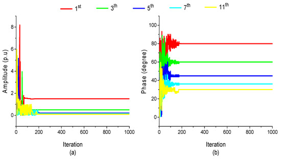
Figure 8.
Variation in estimated (a) amplitude and (b) phase in the course of iterations for the first 5 odd harmonics.
To evaluate the proposed GWO-LS harmonic estimator’s effectiveness, the obtained results are compared with available harmonic estimators in literature, including F-BFO-LS, BFO-RLS, and BBO-RLS GSA-RLS and MABC in terms of percentage error and computational time. The comparison of GWO-LS with literature techniques is tabulated in Table 5. The percentage error of GWO-LS for the 1st, 3rd, 5th, 7th, and 11th harmonic phase are 7.70, 1.48, 6.60, 2.7, and 8.33, respectively. The minimum error is achieved for 1st, 3rd, 5th, 7th, and 11th using GWO-LS in comparison with other harmonic estimators. The comparison between the proposed and literature harmonic estimator in case of harmonics amplitude and phase can be better seen in Figure 9 and Figure 10. It is clear from both the Figures that the proposed GWO-LS estimator has the least percentage error for all the harmonic contents. The behavior of the proposed estimator for approximating frequency components of integral harmonics is demonstrated by Figure 11. It can be clearly seen from Figure 11 that GWO-LS takes a greater number of iterations for estimating frequency than the harmonics amplitude and phase estimation. The proposed harmonic estimators approximate the fundamental frequency in 284 iterations, frequency of 3rd, 5th, 7th, and 11th harmonic in 266, 257, 261, and 276 number of iterations, respectively. It indicates that estimation of fundamental frequency takes higher iterations in case of integral harmonics approximation. It can be concluded form the pictorial and tabular analysis that GWO-LS accurately estimates the frequency components of integral harmonics along with the amplitude and phase of the harmonics.
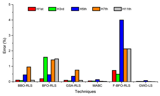
Figure 9.
Comparison of amplitudes error for case study I.
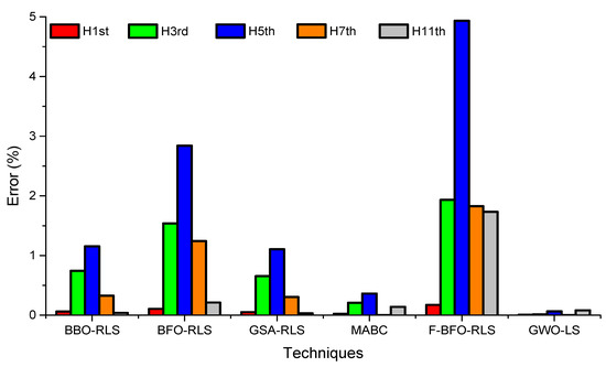
Figure 10.
Comparison of phase errors for case study I.
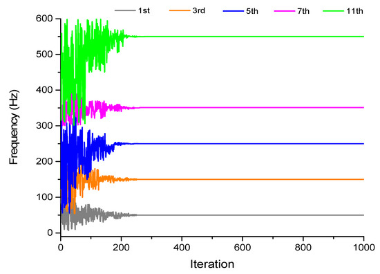
Figure 11.
Frequency estimation for case study I.
Figure 12 demonstrates the GWO-LS behavior for estimating the amplitude of the harmonics in both steady and transient conditions. It is evident from Figure 12 that GWO-LS gives accurate estimation results in steady-state cases while a slight variation is observed for the transient case. The proposed estimator shows estimation variation from 0.17 s to 0.20 s clearly visible in Figure 12b. Similarly, the computational time of GWO-LS to accurately estimate a signal is 0.572 s. It can be observed from Table 5 that the time required to estimate a signal in a noisy environment is minimum for GWO-LS in comparison with all other techniques and it estimates the harmonic amplitudes and phases accurately in the least computational time.
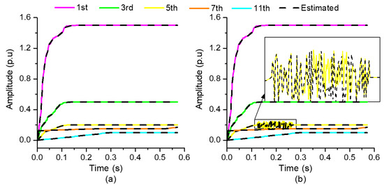
Figure 12.
Estimation in harmonics amplitude (a) steady state condition (b) transient in 5th harmonic.
4.2. Test System II: Estimation of Integral Harmonics Including Sub and Inter Harmonics in a Time-Varying Noisy Environment
In this test system, the power signal is made more complex and distorted by the inclusion of sub and inter harmonics. These sub and inter harmonics have amplitude magnitudes of 0.505, 0.25, and 0.35, respectively, while their phase are 75, 65, and 20, having the frequency of 20, 180, and 230 Hz, respectively [3,38]. The resultant power signal is simulated under both noisy and non-noisy environments. All the other harmonic contents (Amplitudes and phases of integral harmonics) and model evaluation setup remains the same as presented in the previous case study. However, to validate the performance of the presented estimator in approximating dynamic parameters, a short transient is produced in 1st inter harmonic from 0.38 s to 0.5 s.
The numerical values obtained after simulation for this case study are presented in Table 7. If we compare this Table with Table 4 we can see that all values of MSE become higher after considering sub and inter harmonics which indicates that consideration of such harmonics is difficult to estimate. The variation of MSE for the case study for different values of searching agents is presented in Figure 13. It can be seen that the minimum value of MSE is achieved for the 50 number of searching agents. The MSE for this case study is greater than that of case study I due to the inclusion of sub and inter harmonics.
Table 7.
Case Study II Parameters after Simulation.
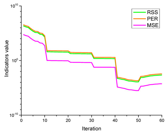
Figure 13.
Searching agents for case study-II.
The pictorial form of the original and estimated signal for the GWO-LS estimator can be seen in Figure 14. It can be observed that the power signal is completely changed after the inclusion of sub and inters harmonics. The GWO-LS estimates the non-noisy and 40 dB signal exactly with great accuracy, as shown in Figure 14. The power signal having 10 dB noise is much difficult to estimate than the others due to higher noise. However, still proposed estimator provides better results than estimators presented in the literature.
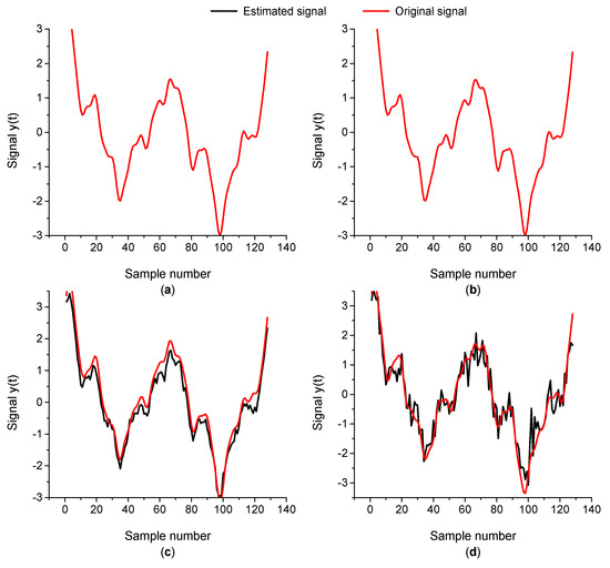
Figure 14.
Actual and Estimated signal comparison (a) non-noisy, (b) 40 dB noise level, (c) 20 dB noise level and (d) 10 dB noise level.
The convergence characteristics for this case study are shown in Figure 15. Figure 15 indicates that the number of iterations to converge increases as the signal’s noise level increases. It is evident from this Figure that the proposed harmonic estimator takes a higher time for the convergence of signal having a higher noise level. Moreover, the presented harmonic estimator takes greater time to converge when compared to case study I. The GWO-LS takes fewer iterations, i.e., 136, to converge for non-noisy signal, but the number of iterations increases with the addition of sub and inter harmonics. GWO-LS takes maximum iterations for 10 dB noisy cases that are 190 iterations.
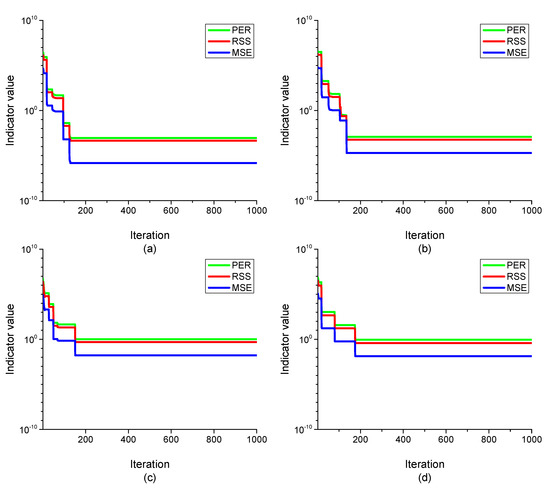
Figure 15.
The convergence characteristics of the GWO-LS framework for case study II (a) non-noisy signal (b) 40 dB (c) 20 dB and (d) 10 dB.
The convergence behavior of GWO-LS estimator for the approximation of sub and inter harmonics over the course of iterations is described in Figure 16. The amplitude and phase of subharmonic take more iteration to converge and more difficult than the amplitude and phase of inter harmonics. Sub and inter harmonics are hard to approximate due to their fractional frequency nature. The amplitudes of subharmonics and second inter harmonic converge in 314 and 323 iterations, while first inter harmonic takes 289 iterations to converge. The phase of sub and inter harmonics converge in 300, 272, and 288 iterations, respectively. The presented estimator takes more iterations to converge for approximating sub and inter harmonics amplitudes and phases than the integral harmonics under time varying noisy environment but still it gives better results than the state of art techniques.
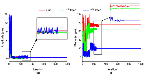
Figure 16.
Variation in estimated (a) amplitude and (b) phase in the course of iterations for the sub and inter harmonics.
The behavior of the proposed estimator for approximating frequency components of sub and inter harmonics is demonstrated by Figure 17. It can be clearly seen from Figure 17 that GWO-LS takes a greater number of iterations for estimating frequency than the harmonics amplitude and phase estimation. The proposed harmonic estimators approximate the sub frequency in 317 iterations, frequency of first and second inter harmonics in 298 and 264 number of iterations, respectively. It reveals that estimation of sub harmonic frequency takes higher iterations while considering all harmonics. Figure 18 demonstrates the GWO-LS behavior for estimating the amplitude of the harmonics in both steady and transient conditions. It is evident from Figure 18 that GWO-LS gives accurate estimation results in steady state cases while a slight variation is observed for the transient case. The proposed estimator shows estimation variation from 0.45 to 0.5 s clearly visible in Figure 18b.
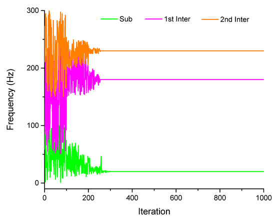
Figure 17.
Frequency estimation for case study II.
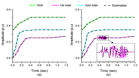
Figure 18.
Estimated harmonic amplitude (a) steady state condition and (b) transient in 1st inter harmonic.
The comparison of the GWO-LS framework with the literature techniques in terms of percentage error between original and approximated harmonic amplitudes and phases is plotted in Figure 19 and Figure 20. Both the Figures demonstrate that the proposed estimator has the minimum percentage error while estimating integral, sub and inter harmonics. Moreover, the comparison of the results of the GWO-LS estimator is also stated in tabular form as Table 6. It is evident from the Table 6 analysis that GWO-LS harmonic estimator is computationally far better than literature estimators by taking 1.17976 s for the approximation of power signal having a sub and inter harmonics. The percentage error between the original harmonic amplitude and phase and the GWO-LS also proved the proposed methodology’s effectiveness. The performance comparison of the presented harmonic estimator with the state of art techniques in terms of performance index also proved the effectiveness of the GWO-LS in the estimation of the sub, inter, and integral harmonics demonstrated in Figure 21 and Table 8. It can be derived from Table 8 and Figure 21 that the proposed estimator has 3.11, 2.61, 1.83 performance indexes for the 40 dB, 20 dB, and 10 dB cases; respectively, which are better than the literature results. Hence, we can conclude that the given harmonic estimator gave promising results in harmonic parameters estimation (sub, inter, and integral harmonics) under a highly noisy and time-varying environment.
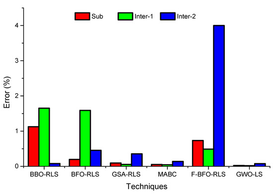
Figure 19.
Comparison of amplitudes erros for case study II.
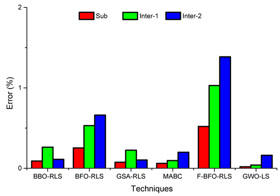
Figure 20.
Comparison of phase error for case study-II.
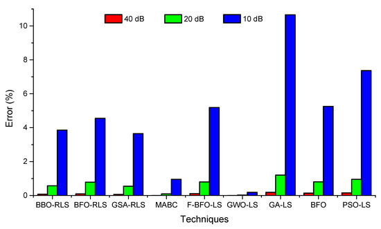
Figure 21.
Comparison of performance index for case study II.
Table 8.
PER comparison of GWO-LS with Literature harmonics estimator for Noisy signals.
5. Conclusions
In this paper, a hybrid harmonic estimator GWO-LS is proposed to estimate harmonics in a power signal. In the proposed harmonic estimator, GWO and LS estimate the non-linear part (phase and frequency) and linear part (amplitude) of a power signal, respectively. For validation of the proposed estimator, two test systems are adopted, among which the first test system contains power harmonics while the second test system considers sub and inter harmonics. Moreover, three different performance indicators are utilized to examine the effectiveness of the proposed approach. The obtained results were compared with recently developed harmonic estimators BFO, F-BFO-LS, ABC-LS, BBO-RLS, GSA-RLS, and MABC. Comparative evaluation of results in terms of percentage error, performance index, and computational time depicts that the proposed GWO-LS estimator estimates the harmonics in a power signal more accurately. The proposed estimator provides less computational complexity, which is essential for the detection of harmonics timely to maintain power quality. The proposed GWO-LS estimator requires 43.5% and 20.6% less time to accurately estimates harmonics in comparison with MABC. Moreover, the obtained percentage error for phase and amplitude indicates that GWO-LS estimates harmonics in a power signal with better accuracy. Furthermore, the proposed estimator accurately estimates harmonics having transient at different time intervals. In addition, the proposed estimator’s PER values are much smaller than the state of art techniques, which clearly verifies that the developed methodology performs the HE problem more accurately and rapidly with a simple structure having fewer controlling parameters.
6. Future Recommendations
- Practical and industrial implementation of proposed research for accurate estimation of electrical harmonics amplitude and phase.
- Proposed harmonic estimator can be helpful in designing active filters to nullify the effects of harmonics thus improving power quality.
- Determine the emission level of higher harmonic components and identifying the source of voltage distortion in the power supply system of industrial enterprises.
- Detailed Analysis of the Steady and transient Conditions of the electrical signals having sub, inter, and integral harmonics.
Author Contributions
Conceptualization and draft writing, M.A.; methodology, T.N.M.; software implementation, A.A.; results validation and formal analysis, M.F.N.; investigation and data curation, I.A.K.; methodology, proofread and edit, R.B. All authors have read and agreed to the published version of the manuscript.
Funding
This research received no external funding.
Data Availability Statement
Not Applicable.
Conflicts of Interest
The authors declare no conflict of interest.
References
- Ahmed, A.; Faisal, M.; Khan, N.; Khan, I.; Member, S.; Alquhayz, H.; Khan, M.A.; Kiani, A.T. A Novel Framework to Determine the Impact of Time Varying Load Models on Wind DG Planning. IEEE Access 2021, 9, 1–16. [Google Scholar] [CrossRef]
- Klyuev, R.V.; Fomenko, O.A.; Gavrina, O.A.; Sokolov, A.A.; Sokolova, O.A.; Dzeranov, B.V.; Morgoev, I.D.; Zaseev, S.G. Analysis of non-sinusoidal voltage at metallurgical enterprises. IOP Conf. Ser. Mater. Sci. Eng. 2019, 663. [Google Scholar] [CrossRef]
- Kabalci, Y.; Kockanat, S.; Kabalci, E. A modified ABC algorithm approach for power system harmonic estimation problems. Electr. Power Syst. Res. 2018, 154, 160–173. [Google Scholar] [CrossRef]
- Hackl, C.M.; Landerer, M. Modified Second-Order Generalized Integrators with Modified Frequency Locked Loop for Fast Harmonics Estimation of Distorted Single-Phase Signals. IEEE Trans. Power Electron. 2020, 35, 3298–3309. [Google Scholar] [CrossRef]
- Ashraf, M.M.; Ullah, M.O.; Malik, T.N.; Waqas, A.B.; Iqbal, M.; Siddiq, F. Robust Extraction of Harmonics using Heuristic Advanced Gravitational Search Algorithm-based Least Square Estimator. Nucleus 2017, 54, 219–231. [Google Scholar]
- Ashraf, M.M.; Ullah, M.O.; Malik, T.N.; Waqas, A.B.; Iqbal, M.; Siddiq, F. A Hybrid Water Cycle Algorithm-Least Square based Framework for Robust Estimation of Harmonics. Nucleus 2018, 55, 47–60. [Google Scholar]
- Labrador Rivas, A.E.; da Silva, N.; Abrão, T. Adaptive current harmonic estimation under fault conditions for smart grid systems. Electr. Power Syst. Res. 2020, 183. [Google Scholar] [CrossRef]
- Enayati, J.; Moravej, Z. Real-time harmonic estimation using a novel hybrid technique for embedded system implementation. Int. Trans. Electr. Energy Syst. 2017, 27, 1–13. [Google Scholar] [CrossRef]
- Yao, J.; Yu, H.; Dietz, M.; Xiao, R.; Chen, S.; Wang, T.; Niu, Q. Acceleration harmonic estimation for a hydraulic shaking table by using particle swarm optimization. Trans. Inst. Meas. Control. 2017, 39, 738–747. [Google Scholar] [CrossRef]
- Chen, C.I.; Chang, G.W. Virtual instrumentation and educational platform for time-varying harmonic and interharmonic detection. IEEE Trans. Ind. Electron. 2010, 57, 3334–3342. [Google Scholar] [CrossRef]
- Urbina-Salas, I.; Razo-Hernandez, J.R.; Granados-Lieberman, D.; Valtierra-Rodriguez, M.; Torres-Fernandez, J.E. Instantaneous Power Quality Indices Based on Single-Sideband Modulation and Wavelet Packet-Hilbert Transform. IEEE Trans. Instrum. Meas. 2017, 66, 1021–1031. [Google Scholar] [CrossRef]
- Jain, S.K.; Singh, S.N. Harmonics estimation in emerging power system: Key issues and challenges. Electr. Power Syst. Res. 2011, 81, 1754–1766. [Google Scholar] [CrossRef]
- Yao, J.; Wan, Z.; Fu, Y. Acceleration Harmonic Estimation in a Hydraulic Shaking Table Using Water Cycle Algorithm. Shock Vib. 2018, 2018. [Google Scholar] [CrossRef]
- Yaghoobi, J.; Alduraibi, A.; Zare, F. Current harmonic estimation techniques based on voltage measurements in distribution networks. Australas. Univ. Power Eng. Conf. AUPEC 2018 2018, 1–6. [Google Scholar] [CrossRef]
- Garanayak, P.; Naayagi, R.T.; Panda, G. A High-Speed Master-Slave ADALINE for Accurate Power System Harmonic and Inter-Harmonic Estimation. IEEE Access 2020, 8, 51918–51932. [Google Scholar] [CrossRef]
- Huang, C.L.; Yang, S.C. Sensorless Vibration Harmonic Estimation of Servo System Based on the Disturbance Torque Observer. IEEE Trans. Ind. Electron. 2020, 67, 2122–2132. [Google Scholar] [CrossRef]
- Rodrigues, N.M.; Ramos, P.M.; Janeiro, F.M. Comparison of harmonic estimation methods for power quality assessment. J. Phys. Conf. Ser. 2018, 1065. [Google Scholar] [CrossRef]
- Malagon-Carvajal, G.; Bello-Pena, J.; Ordonez-Plata, G.; Duarte, C. Time-to-frequency domain SMPS model for harmonic estimation: Methodology. Renew. Energy Power Qual. J. 2017, 1, 825–830. [Google Scholar] [CrossRef]
- Sahu, B.; Dhar, S.; Dash, P.K. Frequency-scaled optimized time-frequency transform for harmonic estimation in photovoltaic-based microgrid. Int. Trans. Electr. Energy Syst. 2020, 30, 1–23. [Google Scholar] [CrossRef]
- Kiani, A.T.; Nadeem, M.F.; Ahmed, A.; Khan, I.; Elavarasan, R.M.; Das, N. Exponential Function-Based Dynamic Inertia Weight Particle Swarm Optimization. Energies 2020, 13, 4037. [Google Scholar] [CrossRef]
- Ahmed, A.; Faisal, M.; Ali, I.; Bo, R.; Khan, I.A. Probabilistic generation model for optimal allocation of wind DG in distribution systems with time varying load models. Sustain. Energy Grids Networks 2020, 22, 100358. [Google Scholar] [CrossRef]
- Ray, P.K.; Subudhi, B. Ensemble-Kalman-filter-based power system harmonic estimation. IEEE Trans. Instrum. Meas. 2012, 61, 3216–3224. [Google Scholar] [CrossRef]
- Singh, S.K.; Sinha, N.; Goswami, A.K.; Sinha, N. Several variants of Kalman Filter algorithm for power system harmonic estimation. Int. J. Electr. Power Energy Syst. 2016, 78, 793–800. [Google Scholar] [CrossRef]
- Karimi-Ghartemani, M.; Ooi, B.T.; Bakhshai, A. Application of enhanced phase-locked loop system to the computation of synchrophasors. IEEE Trans. Power Deliv. 2011, 26, 22–32. [Google Scholar] [CrossRef]
- Xi, Y.; Tang, X.; Li, Z.; Cui, Y.; Zhao, T.; Zeng, X.; Guo, J.; Duan, W. Harmonic estimation in power systems using an optimised adaptive Kalman filter based on PSO-GA. IET Gener. Transm. Distrib. 2019, 13, 3968–3979. [Google Scholar] [CrossRef]
- Durdhavale, S.R.; Ahire, D.D. A Review of Harmonics Detection and Measurement in Power System. Int. J. Comput. Appl. 2016, 143, 975–8887. [Google Scholar]
- Lu, Z.; Ji, T.Y.; Tang, W.H.; Wu, Q.H. Optimal harmonic estimation using a particle swarm optimizer. IEEE Trans. Power Deliv. 2008, 23, 1166–1174. [Google Scholar] [CrossRef]
- Kiani, A.T.; Nadeem, M.F.; Ahmed, A.; Sajjad, I.A.; Haris, M.S.; Martirano, L. Optimal Parameter Estimation of Solar Cell using Simulated Annealing Inertia Weight Particle Swarm Optimization (SAIW-PSO). In Proceedings of the 2020 IEEE International Conference on Environment and Electrical Engineering and 2020 IEEE Industrial and Commercial Power Systems Europe (EEEIC/I&CPS Europe), Madrid, Spain, 9–12 June 2020; IEEE: Piscataway, NJ, USA, 2020; pp. 1–6. [Google Scholar] [CrossRef]
- Bettayeb, M.; Qidwai, U. A hybrid least squares-GA-based algorithm for harmonic estimation. IEEE Trans. Power Deliv. 2003, 18, 377–382. [Google Scholar] [CrossRef]
- Mishra, S. Hybrid least-square adaptive bacterial foraging strategy for harmonic estimation. IEE Proc. Gener. Transm. Distrib. 2005, 152, 379–389. [Google Scholar] [CrossRef]
- Subudhi, B.; Ray, P.K. A hybrid Adaline and Bacterial Foraging approach to power system harmonics estimation. In Proceedings of the 2010 International Conference on Industrial Electronics, Control and Robotics, Rourkela, India, 27–29 December 2010; IEEE: Piscataway, NJ, USA, 2010; pp. 236–242. [Google Scholar] [CrossRef]
- Ji, T.Y.; Li, M.S.; Wu, Q.H.; Jiang, L. Optimal estimation of harmonics in a dynamic environment using an adaptive bacterial swarming algorithm. IET Gener. Transm. Distrib. 2011, 5, 609–620. [Google Scholar] [CrossRef]
- Singh, S.K.; Sinha, N.; Goswami, A.K.; Sinha, N. Optimal estimation of power system harmonics using a hybrid Firefly algorithm-based least square method. Soft Comput. 2017, 21, 1721–1734. [Google Scholar] [CrossRef]
- Biswas, S.; Chatterjee, A.; Goswami, S.K. An artificial bee colony-least square algorithm for solving harmonic estimation problems. Appl. Soft Comput. J. 2013, 13, 2343–2355. [Google Scholar] [CrossRef]
- Singh, S.K.; Sinha, N.; Goswami, A.K.; Sinha, N. Power system harmonic estimation using biogeography hybridized recursive least square algorithm. Int. J. Electr. Power Energy Syst. 2016, 83, 219–228. [Google Scholar] [CrossRef]
- Kabalci, Y.; Kockanat, S.; Kabalci, E. A differential search algorithm application for solving harmonic estimation problems. In Proceedings of the 2017 9th International Conference on Electronics, Computers and Artificial Intelligence (ECAI), Targoviste, Romania, 29 June–1 July 2017; pp. 1–5. [Google Scholar] [CrossRef]
- Singh, S.K.; Kumari, D.; Sinha, N.; Goswami, A.K.; Sinha, N. Gravity Search Algorithm hybridized Recursive Least Square method for power system harmonic estimation. Eng. Sci. Technol. Int. J. 2017, 20, 874–884. [Google Scholar] [CrossRef]
- Xu, Y.; Liu, Y.; Li, Z.; Li, Z.; Wang, Q. Harmonic estimation base on center frequency shift algorithm. Mapan J. Metrol. Soc. India 2017, 32, 43–50. [Google Scholar] [CrossRef]
- Saxena, A.; Kumar, R.; Mirjalili, S. A harmonic estimator design with evolutionary operators equipped grey wolf optimizer. Expert Syst. Appl. 2020, 145, 113125. [Google Scholar] [CrossRef]
- Carbajal, F.B.; Olvera, R.T. An adaptive neural online estimation approach of harmonic components. Electr. Power Syst. Res. 2020, 186, 106406. [Google Scholar] [CrossRef]
- Cupertino, F.; Lavopa, E.; Zanchetta, P.; Sumner, M.; Salvatore, L. Running DFT-based PLL algorithm for frequency, phase, and amplitude tracking in aircraft electrical systems. IEEE Trans. Ind. Electron. 2011, 58, 1027–1035. [Google Scholar] [CrossRef]
- Mirjalili, S.; Mirjalili, S.M.; Lewis, A. Grey Wolf Optimizer 1 1. Adv. Eng. Softw. 2014, 69, 46–61. [Google Scholar] [CrossRef]
- Li, Y.; Deng, Z.; Wang, T.; Zhao, G.; Zhou, S. Coupled harmonic admittance identification based on least square estimation. Energies 2018, 11, 2600. [Google Scholar] [CrossRef]


Publisher’s Note: MDPI stays neutral with regard to jurisdictional claims in published maps and institutional affiliations. |
© 2021 by the authors. Licensee MDPI, Basel, Switzerland. This article is an open access article distributed under the terms and conditions of the Creative Commons Attribution (CC BY) license (https://creativecommons.org/licenses/by/4.0/).