New Methodology for Computing the Aircraft’s Position Based on the PPP Method in GPS and GLONASS Systems

Abstract

In the field of air navigation, there is a constant pursuit for new navigation solutions for precise GNSS (Global Navigation Satellite System) positioning of aircraft. This study aims to present the results of research on the development of a new method for improving the performance of PPP (Precise Point Positioning) positioning in the GPS (Global Positioning System) and GLONASS (Globalnaja Nawigacionnaja Sputnikovaya Sistema) systems for air navigation. The research method is based on a linear combination of individual position solutions from the GPS and GLONASS systems. The paper shows a computational scheme based on the linear combination for geocentric XYZ coordinates of an aircraft. The algorithm of the new research method uses the weighted mean method to determine the resultant aircraft position. The research method was tested on GPS and GLONASS kinematic data from an airborne experiment carried out with a Seneca Piper PA34-200T aircraft at the Mielec airport. A dual-frequency dual-system GPS/GLONASS receiver was placed on-board the plane, which made it possible to record GNSS observations, which were then used to calculate the aircraft’s position in CSRS-PPP software. The calculated XYZ position coordinates from the CSRS-PPP software were then used in the weighted mean model’s developed optimization algorithm. The measurement weights are a function of the number of GPS and GLONASS satellites and the inverse of the mean error square. The obtained coordinates of aircraft from the research model were verified with the RTK-OTF solution. As a result of the research, the presented solution’s accuracy is better by 11–87% for the model with a weighting scheme as a function of the inverse of the mean error square. Moreover, using the XYZ position from the RTKLIB program, the research method’s accuracy increases from 45% to 82% for the model with a weighting scheme as a function of the inverse of the square of mean error. The developed method demonstrates high efficiency for improving the performance of GPS and GLONASS solutions for the PPP measurement technology in air navigation.

1. Introduction

To date, the trend of using GNSS (Global Navigation Satellite System) satellite technology in aviation has been exclusively based on single-frequency receivers, recording the publicly available L1-C/A code measurement. Consequently, ICAO (International Civil Aviation Organization) technical standards in the aspect of quality of GNSS positioning in aviation are referred to the L1 frequency [1]. Thus, for many years, only GNSS L1-C/A code observations were used in flight tests to determine the accuracy, reliability, continuity and availability of the aircraft navigation solution. However, the development of GNSS satellite receiver technology and the growth of the GNSS space segment made it possible to use observations on the other carrier frequencies as well. In practice, the use of GNSS dual-frequency observations in navigation calculations adds value to the aircraft position determination process.

For GNSS satellite observations, we distinguish both absolute and differential (relative) positioning methods in navigation calculations [2]. Among the absolute positioning methods, one of the precise measurement techniques is the dual-frequency PPP (Precise Point Positioning) method [3]. The PPP measurement technique uses code observations (P1 and P2) and phase observations (L1 and L2) from a dual-frequency GNSS satellite receiver on-board the aircraft [3]. Thus, during the flight operation, the aircraft crew should be equipped only with a dual-frequency GNSS receiver for precise computation of the aircraft flight path using the PPP method. A completely different situation occurs in the case of differential positioning, where the differential RTK (Real-Time Kinematic) technique with an OTF (On The Fly) solution for GNSS phase measurements is used as a precise measurement technique [4]. The differential RTK technique uses a GNSS satellite receiver on-board the aircraft and a GNSS satellite receiver installed at the reference station (base station) [5]. The differential RTK technique requires the use of a minimum of two GNSS satellite receivers, which, in turn, translates into increased costs and the need to purchase technical infrastructure. In order to reduce the financial costs and the number of personnel to operate the GNSS reference station infrastructure, the PPP measurement technique is increasingly used in flight tests.

The common feature of the absolute PPP method and the differential RTK technique is their use to determine an aircraft’s reference position in flight tests. Consequently, both measurement methods are significant for the problem of determining the true trajectory of an aircraft determined from dual-frequency GNSS observations. Knowing the aircraft’s true position is essential for both pilots and air traffic ground personnel, including controllers and navigators.

2. Related Papers

The problem of determining an aircraft’s actual position using the PPP method has been presented and described in many research papers worldwide. Most research papers on PPP positioning in air navigation had described and presented position solutions using GPS (Global Positioning System) or GLONASS (Globalnaja Nawigacionnaja Sputnikovaya Sistema) navigation systems. That is, of course, related to the fact that only GPS and GLONASS systems are certified by ICAO for GNSS satellite navigation in aviation [1]. It can be concluded that GPS and GLONASS, as global GNSS navigation systems, provide continuous satellite positioning in aviation.

The literature review provides a multi-faceted approach to the application of the PPP measurement technique in air navigation. Reference [6] propose using a PPP solution to determine the position of an aircraft with respect to the differential solution from the AUSPOS program. The aircraft’s position was determined in the CSRS-PPP (Canadian Spatial Reference System–Precise Point Positioning) program using the least-squares method for GPS observations. The maximum coordinate difference between the GAPS (GPS Analysis and Positioning Software) and AUSPOS (online GPS processing service) solution was up to ±0.5 m for the horizontal coordinates and ±1 m for the vertical coordinate. In turn, the paper [7] proposed the use of a PPP solution to determine the position of a helicopter with respect to a DD (Double Difference) differential solution in postprocessing. The helicopter position was determined in the P3 (software developed by the University of Calgary) software package using Kalman filtering for GPS observations. The maximum coordinate difference between the PPP solution and the differential DD solution reached ±0.5 m for all ENU (East-North-Up) components. A similar solution was proposed in work [8], in which helicopter positioning accuracy was determined using the P3 (software developed by the University of Calgary) software package with the PPP method. The initial positioning accuracy of the helicopter was about 2.7 m, while, in the final phase of the flight, it was higher than 0.1 m for BLh (B: Latitude, L: Longitude and h: ellipsoidal height) coordinates. In paper [9], P3 software was used to determine the positioning accuracy of an aircraft flying at high speed. The values of positioning errors of the aircraft between the PPP solution and the differential DD solution were up to ±0.2 m for the horizontal coordinates and ±1.1 m for the vertical coordinate. However, paper [10] used the PPP method to determine a helicopter’s position with respect to the KGPS (Kinematic GPS) solution in the PNAV program. The helicopter position was determined using Kalman filtering for GPS observations. The maximum coordinate difference between the PPP solution and the KGPS PNAV solution was up to ±1 m for all ENU components. Furthermore, in work [11], the PPP method was used to determine the UAV (Unmanned Aerial Vehicle) position in GIPSY and RTKLIB software. The UAV reference position was determined using the DGPS (Differential GPS) technique for GPS phase observations. The paper presents different scenarios for UAV position determination for the PPP method: iterative method, filtering of GPS observations and the smoothing of code observations by GPS phase observations. The maximum coordinate difference between the PPP and DGPS solutions reached ±1 m for all ENU components. In paper [12], the PPP method’s accuracy in PP-RTX software was investigated in more than 100 flight tests. The PP-RTX solution’s typical accuracy with respect to the ASB (Applanix Smartbase) differential solution was up to ±0.2 m for all ENU components. In turn, the paper [13] proposed to test the PPP method in TriP, IT and GrafNav software in a flight experiment. This paper presented the results of the comparison of the aircraft coordinate determination between the TriP, IT, GrafNav software and the GPSurvey baseline solution. The typical positioning accuracy of the aircraft from the PPP method was up to ±0.7 m for all ENU components. On the other hand, the paper [14] presented the results of the positioning accuracy of the aircraft from the CSRS-PPP and GrafNav solutions concerning the DD differential solution. The average positioning accuracy from the PPP method was ±0.2 ÷ 0.4 m; however, numerous anomalies can be observed from the GrafNav solution when the accuracy decreases to the level of ±1.5 m. Interesting solutions for applying the PPP method for single-frequency GPS receivers were presented in papers [15,16]. The papers described the application of the method of smoothing code measurements with GPS phase measurements using IGS (International GNSS Service) products in air navigation. The typical GPS positioning accuracy for the PPP method in works [15,16] was about ±1 m for all ENU and BLh frame components. Another very interesting solution for the needs of aerial photogrammetry was the application of the PPP method in the process of digital aerotriangulation in the works [17,18]. The PPP method was used to determine the UAV position during the photogrammetric flight. The obtained PPP positioning accuracy was higher than ±0.3 m in [17] and higher than ±1.2 m in [19] in the ENU coordinate frame. The use of the PPP method in air navigation allowed for combining navigation solutions using different sensors, e.g., a GNSS receiver and an INS (Inertial Navigation System) system. The works [19,20,21,22] presented a combined solution of aircraft positioning using the PPP/INS method in relation to the differential GPS RTK solution. The obtained PPP/INS positioning accuracy was: higher than ±0.2 m in [19], higher than ±0.4 m in work [20] and higher than ±0.1 m in [21,22]. In paper [23], the IGS and CNES (Centre National d’Etudes Spatiales) Analysis Center products were applied in aerial triangulation and, also, to determine the coordinates of an airplane.

During in-flight tests in Poland, the PPP measurement technique has not been widely used as an aircraft flight reference position so far. An example of testing the vertical plane’s actual flight trajectory was described in the paper [24]. In the previous flight experiments in Poland, the differential RTK technique in the OTF mode was used as the aircraft reference position. Such a solution was proposed, and in-flight tests described, among others, in research papers [25,26,27]. Therefore, in Polish scientific research, there is a lack of confirmation and verification of the PPP measurement method as an alternative measurement technique to determine the aircraft’s real trajectory. The use of the PPP method in flight tests in Poland has been limited only to testing the precision of determining aircraft coordinates [3,28,29]. Moreover, in works [30,31], the PPP method was used to determine the aircraft’s precise trajectory to test the accuracy of SPP (Single-Point Positioning) code positioning in air navigation in Polish aviation. It is worth mentioning that the PPP method was used in air navigation in Poland for positioning using the GLONASS navigation system. Thus, paper [32] presented a model for determining the position of a Cessna-172 aircraft using GLONASS observations in the CSRS-PPP program. In turn, paper [33] presented the results of GLONASS positioning in the PPP method in relation to the joint GPS/GLONASS solution in the RTKLIB program. Furthermore, paper [34] presented the results of PPP positioning in GLONASS from RTKLIB and CSRS-PPP solution.

The research problem of using the PPP method in air navigation, discussed in this paper, concerns both real-time positioning and post-processing mode. The presented publications [6,7,8,9,10,11,12,13,14,15,16,17,18,19,20,21,22,23,24,25,26,27,28,29,30,31,32,33] presented research works both in real-time and post-processing mode. Therefore, the PPP positioning problem in air navigation is dual, i.e., it concerns real-time applications and the post-processing mode. The use of both is crucial and has its properties. In real-time, this is a navigation domain and allows the user to read real-time positions using the PPP method. The pilot must have confidence and credibility in the computer software that performs the calculations, and above all, the software must be tested and validated for air navigation. On the other hand, post-processing for the PPP method is primarily a post-factum analysis of the determined plane coordinates, reduction of systematic errors, detection of outliers, etc. All this is reflected in the objective flight control laboratory. Therefore, in the case of the PPP method, application tools must be designed for real-time and post-processing calculations.

Based on the accumulated literature on PPP positioning in air navigation, it can be observed that research studies have used a solution from a single GNSS navigation system such as GPS or GLONASS. This raises the research problem of what optimal computational strategy to use to improve a single GPS or GLONASS PPP solution relative to a RTK GNSS solution. Thus, an optimization algorithm should be used to improve the performance of PPP positioning in GPS or GLONASS in air navigation. One way to solve this problem is to create a linear combination of the determined coordinates from the PPP GPS and PPP GLONASS methods. This solution will determine the relationship between individual PPP GPS and PPP GLONASS solutions in relation to the RTK GNSS solution. Moreover, this approach shows how to choose the optimal weighting strategy to integrate GPS/GLONASS solutions in the PPP method. The weighted model gives an additional one degree of freedom to solve the plane’s accidental position for independent GPS and GLONASS data. Moreover, in such an approach, measurement scales may be selected further to increase the air navigation PPP method’s positioning accuracy. The weighted average model is characterized by high efficiency and effectiveness in improving coordinates’ performance with appropriate selection of measuring weights [35].

The presented paper aims to show a new computational strategy for PPP positioning in air navigation for a single GPS and GLONASS solution. For this purpose, the development of a new boundary condition combining single GPS and GLONASS solutions in the PPP method is proposed. This condition is based on the weighted mean model. The proposed algorithm was tested on GPS and GLONASS kinematic data from an airborne experiment carried out with a Seneca Piper PA34-200T aircraft at a civil airport in Mielec, Poland. The presented numerical solution was performed in Scilab based on the aircraft position results obtained from CSRS-PPP. The presented results are unique for the application of the PPP method in Polish aviation.

3. Research Method

This section shows the PPP positioning algorithm for a single GPS and GLONASS solution. Additionally, a new PPP positioning algorithm improving the GPS and GLONASS single solution is presented.

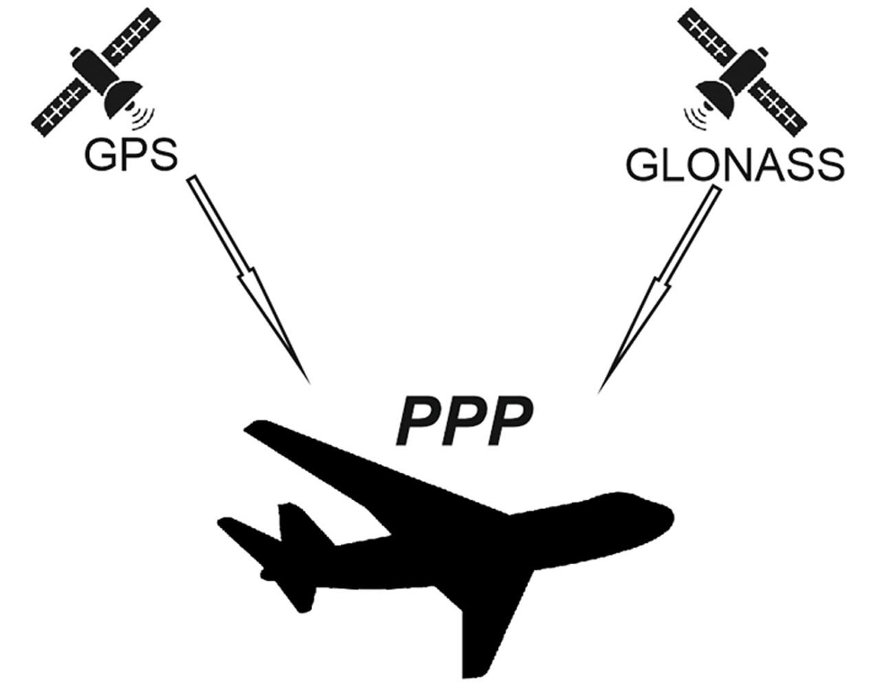
3.1. Positioning Model of the PPP Method for GPS and GLONASS Solutions

The basic observation equation of the PPP measurement technique can be written as follows [33,34,36]:

-

for GPS or GLONASS:

$$\{\begin{array}{l}{P}_3=d+c·\left(dtr-dts\right)+Trop+Rel+M_{P3}\\ L_3=d+c·\left(dtr-dts\right)+Trop+B_3+Rel+\delta w+M_{L3 }\end{array}$$

(1)

where:

P₃ and L₃—observation equations of the GPS or GLONASS linear Ionosphere-Free combination;

P₃ = α·P₁ + β·P₂;

L₃ = α·L₁ + β·L₂;

(P₁, P₂)—GPS or GLONASS code observations;

(L₁, L₂)—GPS or GLONASS phase observations;

α = +f₁²/(f₁² − f₂²), GPS or GLONASS linear coefficient;

β = −f₂²/(f₁² − f₂²), GPS or GLONASS linear coefficient;

(f₁, f₂)—frequencies of the GPS or GLONASS signals;

d—geometric satellite-receiver distance in GPS or GLONASS system; takes into account the phase centre characteristics of the satellite antenna and the receiver [37],

$$d=\sqrt{{\left(X_{}^r-X_{}^s\right)}^2+{\left(Y_{}^r-Y_{}^s\right)}^2+{\left(Z_{}^r-Z_{}^s\right)}^2}$$

(2)

($X_{}^r$,$Y_{}^r$,$Z_{}^r$)—XYZ geocentric coordinates of the aircraft;

($X_{}^s$,$Y_{}^s$,$Z_{}^s$)—orbital coordinates of the GPS or GLONASS satellite;

c—the speed of light;

dtr—correction of the receiver’s clock in the GPS or GLONASS system;

dts—correction of the satellite’s clock in the GPS or GLONASS system;

Trop—Tropospheric delay in GPS or GLONASS measurements;

Trop = SWD + SHD;

SHD—slant path tropospheric delay for the hydrostatic component;

SWD—slant path tropospheric delay for the wet component;

SHD = mf_H·ZHD;

SWD = mf_W·ZWD;

(mf_H, mf_W)—mapping functions for the hydrostatic and wet paths of the tropospheric delay;

ZHD—hydrostatic component of tropospheric delay;

ZWD—wet component of tropospheric delay;

Rel—relativistic effects in GPS or GLONASS measurements;

B₃—float value of phase ambiguity in GPS or GLONASS measurements;

δw—phase wind-up in GPS or GLONASS system;

M_P3—multipath effect of GPS or GLONASS code observations;

M_L3—multipath effect of GPS or GLONASS phase observations.

The unknown parameters in the PPP measurement technique in the GPS and GLONASS solutions are, respectively [38], residuals to the approximate coordinates of the receiver $[\delta X,\delta Y,\delta Z]$, the receiver’s clock correction $dtr$, phase ambiguities $B_3$ (determined for each visible GPS and GLONASS satellite) and the wet component of the tropospheric delay $ZWD$. The above-mentioned unknown parameters are determined by the least-squares method in a sequential stochastic process in GPS and GLONASS systems, respectively, as follows [39]:

$$Sx={\left(A_{}^T\cdot P\cdot A+C_x^{-1}\right)}^{-1}{A}_{}^T\cdot P\cdot l$$

(3)

where:

$Sx$—vector of the unknown parameters,

$A$—design matrix,

$$A=\left[\begin{array}{cccccccccc}\frac{X_{i-1}^r-X_{}^s}{d_{i-1}}& \frac{Y_{i-1}^r-Y_{}^s}{d_{i-1}}& \frac{Z_{i-1}^r-Z_{}^s}{d_{i-1}}& 1& 0& 0& \dots & \dots & \dots & m{f}_W\\ \dots & \dots & \dots & 1& 1& 0& \dots & \dots & \dots & \dots \\ \dots & \dots & \dots & 1& 0& 0& \dots & \dots & \dots & \dots \\ \dots & \dots & \dots & 1& 0& 1& \dots & \dots & \dots & \dots \\ \dots & \dots & \dots & 1& 0& 0& \dots & 0& 0& \dots \\ \dots & \dots & \dots & \dots & \dots & \dots & \dots & 1& 0& \dots \\ \dots & \dots & \dots & \dots & \dots & \dots & \dots & 0& 0& \dots \\ \dots & \dots & \dots & 1& 0& 0& \dots & 0& 1& m{f}_W\end{array}\right]$$

(4)

$(X_{i-1}^r,Y_{i-1}^r,Z_{i-1}^r,)$—geocentric XYZ coordinates of the aircraft per observation time epoch $(i-1)$,

$(i-1)$—previous observation time epoch,

$d_{i-1}$—approximately the geometric satellite-receiver distance in GPS or GLONASS system;

$P$—matrix of weights,

$C_x^{}$—variance-covariance matrix,

$C_x={\left(A_{}^T\cdot P\cdot A+C_x^{-1}\right)}^{-1}+C_n$,

$C_n$—the process disturbance noise matrix,

$l$—vector of difference between observations and modelled parameters.

The final aircraft coordinates from the PPP method from the GPS or GLONASS solutions are determined as recorded below [40]:

$$\{\begin{array}{c}{X}_i^r=X_{i-1}^r+\delta X_{}\\ Y_i^r=Y_{i-1}^r+\delta Y_{}\\ Z_i^r=Z_{i-1}^r+\delta Z_{}\end{array}$$

(5)

where:

$(X_i^r,Y_i^r,Z_i^r)$—geocentric XYZ coordinates of the aircraft per observation time epoch $(i)$, and $(i)$—the current observation time epoch.

3.2. New Mathematical Scheme for Improving the GPS and GLONASS Solution in the PPP Method

The new concept of PPP positioning from the GPS and GLONASS solution was based on the resultant linear combination model in which weighting factors $(a,b,c,d,e,f)$ were used. In the new approach, the aircraft’s resultant position is determined in geocentric XYZ coordinates based on a single PPP GPS and PPP GLONASS solution. The new algorithm’s goal is to determine the best match between the PPP GPS and PPP GLONASS solution relative to the flight reference position calculated from the differential RTK technique. Moreover, the proposed algorithm determines the most optimal solution of the resultant position of the aircraft, i.e., it will be checked which measuring scales improve the performance of determining the resultant aircraft coordinates. The proposed calculation scheme of the resultant position of the aircraft is described below:

$$\{\begin{array}{c}{X}_k=\frac{a\cdot X_g+b\cdot X_r}{a+b}\\ Y_k=\frac{c\cdot Y_g+d\cdot Y}{c+d}\\ Z_k=\frac{e\cdot Z_g+f\cdot Z_r}{e+f}\end{array}$$

(6)

where:

$X_g=X_i^r$ (see Equation (3)), position of aircraft from GPS solution along X axis,

$Y_g=Y_i^r$ (see Equation (3)), position of aircraft from GPS solution along Y axis,

$Z_g=Z_i^r$ (see Equation (3)), position of aircraft from GPS solution along Z axis,

$X_r=X_i^r$ (see Equation (3)), position of aircraft from GLONASS solution along X axis,

$Y_r=Y_i^r$ (see Equation (3)), position of aircraft from GLONASS solution along Y axis,

$Z_r=Z_i^r$ (see Equation (3)), position of aircraft from GLONASS solution along Z axis,

$(a,b,c,d,e,f)$—determined linear coefficients, dimensionless values,

$(X_k^{},Y_k^{},Z_k^{})$—resultant position of aircraft.

Equation (4) combines 2 independent GPS and GLONASS determinations of the aircraft position using the PPP method. In this way, the aircraft’s resultant position is determined every given measurement epoch, typically in the time interval of 1 s. It should be noted that the critical parameters in Equation (4) are the values of linear coefficients. In the analyzed example, a weighting scheme based on the following weighting factors was proposed:

$$\{\begin{array}{c}a=c=e=\frac{1}{n{s}_g}\vee a=c=e=\frac{1}{C{l}_g^2}\\ b=d=f=\frac{1}{n{s}_r}\vee b=d=f=\frac{1}{C{l}_r^2}\end{array}$$

(7)

where:

$n{s}_g$—number of GPS satellites,

$n{s}_r$—number of GLONASS satellites,

$C{l}_g$—mean error of the determined coordinates from the PPP GPS solution,

$C{l}_r$—mean error of the determined coordinates from the PPP GLONASS solution.

The calculation process of determining the resultant position of the aircraft according to Equation (4) uses weighting factors $(a,b,c,d,e,f)$. In the analyzed model, two approaches for determining the weighting factors $(a,b,c,d,e,f)$ were proposed. The first approach is based on a weighing scale as a function of the reciprocal of the number of GPS or GLONASS satellites. On the other hand, the second approach is based on the measurement weight as a function of the inverse of the square of the mean coordinate errors of the aircraft from the PPP GPS and PPP GLONASS solutions. On this basis, it is possible to optimize the calculation process of the aircraft’s resultant position. It means that based on Equation(4), the resultant plane position for the PPP method will be calculated, and by the way, it will be shown which measurement weight is the best for this type of mathematical model, as in Equation (4). That is important, because we are looking for mathematical models in air navigation to improve the aircraft’s position. All the more, determining the appropriate measurement weight here is crucial to improving the accuracy of PPP positioning in aeronautical navigation.

The algorithm for determining the values in the $C{l}_g$ and $C{l}_r$ parameters is described below [41]:

$$\{\begin{array}{c}\frac{1}{C{l}_g^2}=\frac{1}{m{x}_g^2+m{y}_g^2+m{z}_g^2}\\ \frac{1}{C{l}_r^2}=\frac{1}{m{x}_r^2+m{y}_r^2+m{z}_r^2}\end{array}$$

(8)

where:

$(m{x}_g,m{y}_g,m{z}_g)$—mean coordinate errors determined from the GPS variance–covariance matrix $C_x^{}$ (see Equation (2)),

$\{\begin{array}{c}m{x}_g=C_x(1,1)\\ m{y}_g=C_x(2,2)\\ m{z}_g=C_x(3,3)\end{array}\begin{array}{c}\end{array}from\begin{array}{c}\end{array}PPP\begin{array}{c}\end{array}GPS\begin{array}{c}\end{array}solution$ (see Equation (2)),

$(m{x}_r,m{y}_r,m{z}_r)$—mean coordinate errors determined from the GLONASS variance–covariance matrix $C_x^{}$ (see Equation (2)),

$\{\begin{array}{c}m{x}_r=C_x(1,1)\\ m{y}_r=C_x^{}(2,2)\\ m{z}_r=C_x(3,3)\end{array}\begin{array}{c}\end{array}from\begin{array}{c}\end{array}PPP\begin{array}{c}\end{array}GLONASS\begin{array}{c}\end{array}solution$ (see Equation (2)).

In the next step, additional parameters for the resultant position of the aircraft were determined, i.e.,

-

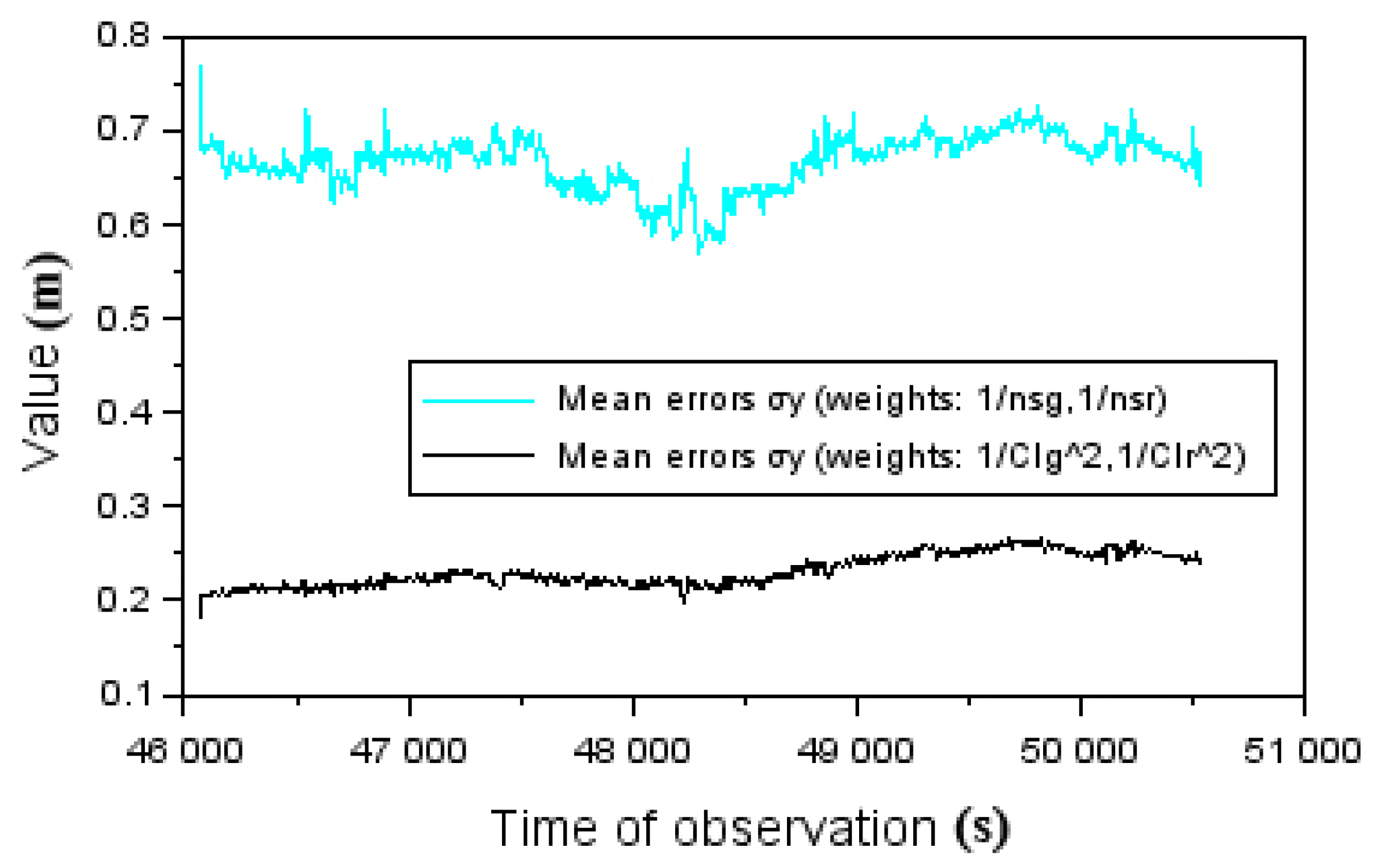
determination of the average measurement error,

-

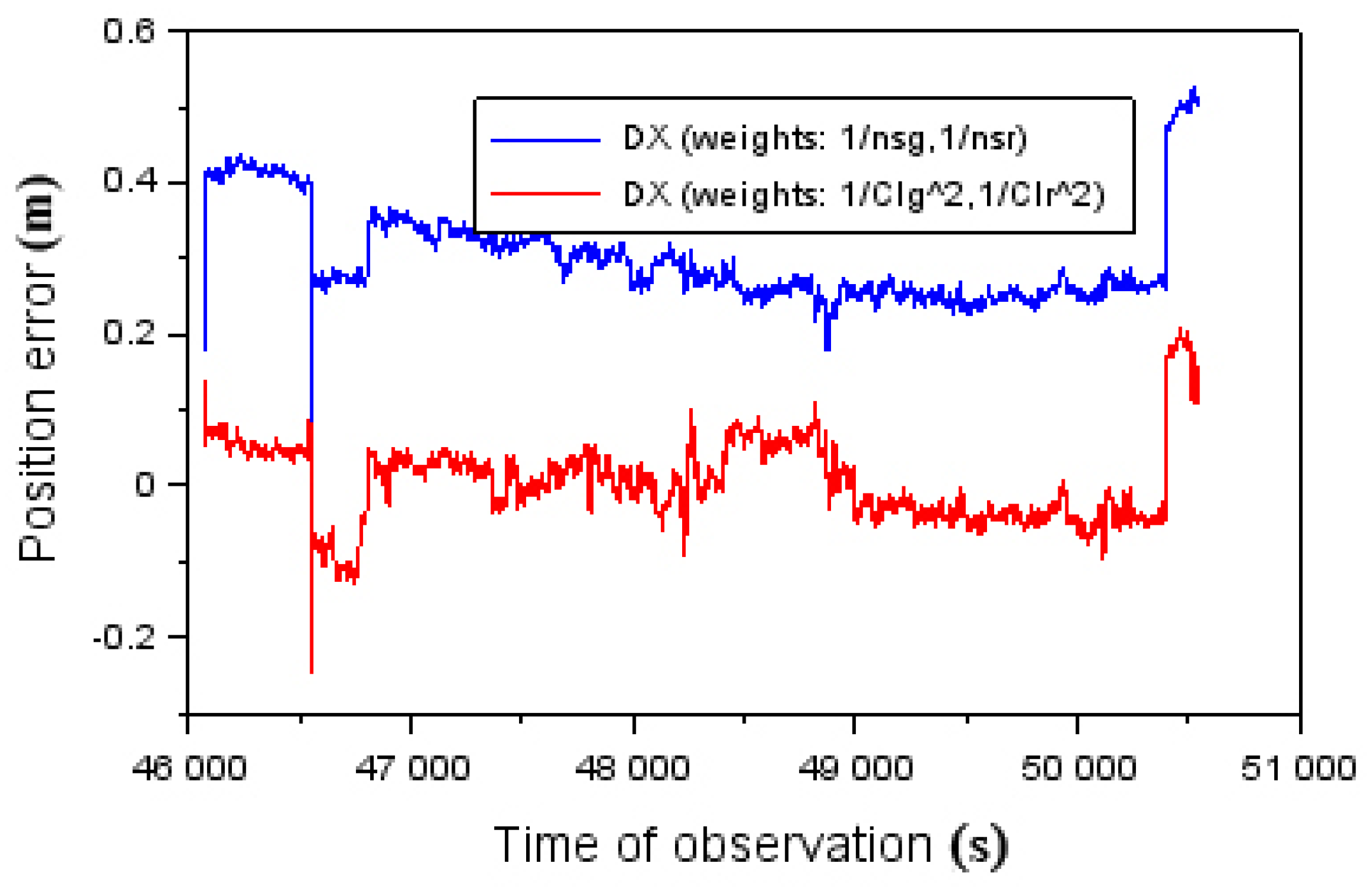
determining the corrections,

-

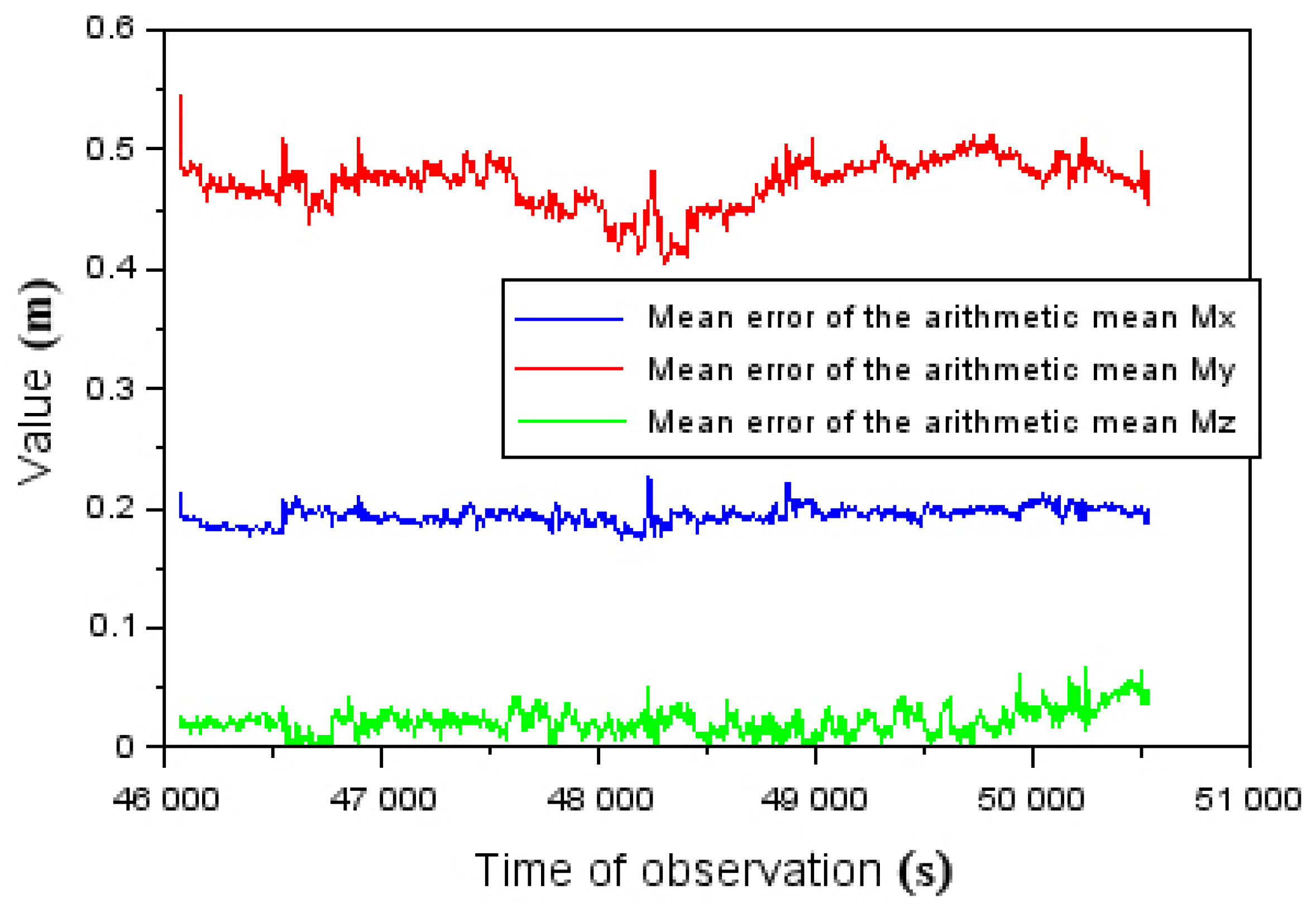
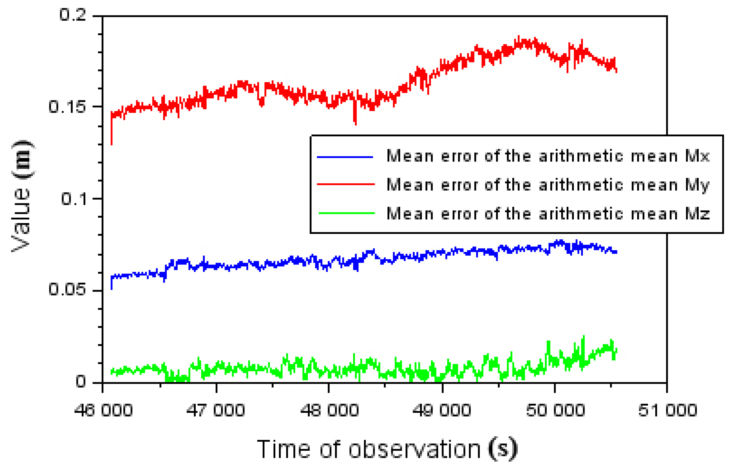
determination of the mean error of the arithmetic mean.

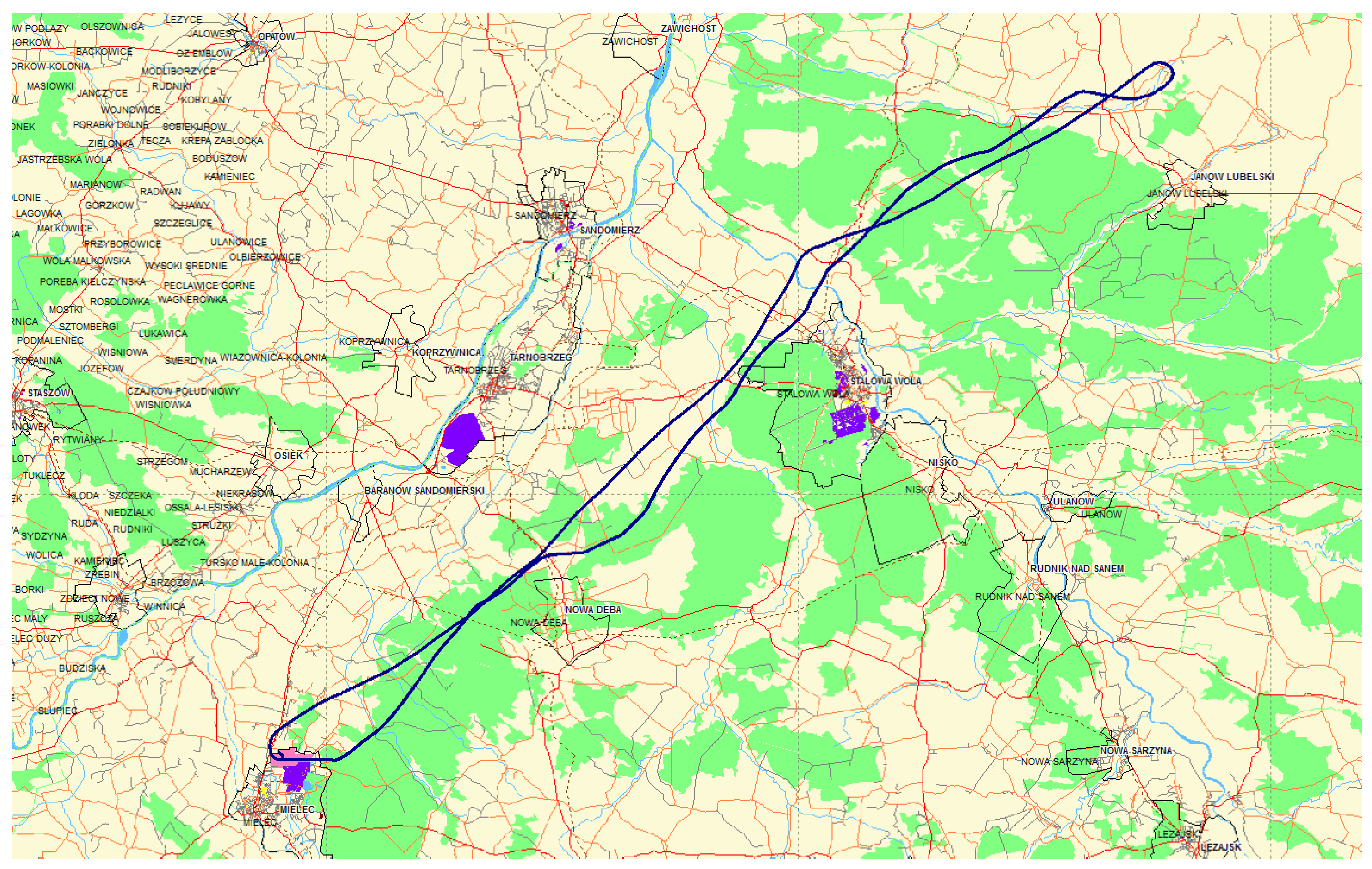
The scheme of the procedure for this stage was written in Equation (7):

$$\{\begin{array}{l}{V}_g=\{\begin{array}{c}{V}_{g,x}=X_g-X_k\\ V_{g,y}=Y_g-Y_k\\ V_{g,z}=Z_g-Z_k\end{array}\\ V_r=\{\begin{array}{c}{V}_{r,x}=X_r-X_k\\ V_{r,y}=Y_r-Y_k\\ V_{r,z}=Z_r-Z_k\end{array}\\ {\sigma }_x=\sqrt{\frac{\left[V_{g,x}^T\cdot P_g\cdot V_{g,x}+V_{r,x}^T\cdot P_r\cdot V_{r,x}\right]}{n-1}}\\ {\sigma }_y=\sqrt{\frac{\left[V_{g,y}^T\cdot P_g\cdot V_{g,y}+V_{r,y}^T\cdot P_r\cdot V_{r,y}\right]}{n-1}}\\ {\sigma }_z=\sqrt{\frac{\left[V_{g,z}^T\cdot P_g\cdot V_{g,z}+V_{r,z}^T\cdot P_r\cdot V_{r,z}\right]}{n-1}}\\ M_x=\frac{{\sigma }_x}{\sqrt{n}}\\ M_y=\frac{{\sigma }_y}{\sqrt{n}}\\ M_z=\frac{{\sigma }_z}{\sqrt{n}}\end{array}$$

(9)

where:

$P_g$—matrix of weights for PPP GPS solution, $P_g=\frac{1}{n{s}_g}\begin{array}{c}\end{array}\vee \begin{array}{c}\end{array}{P}_g=\frac{1}{C{l}_g^2}$ (see Equation (5)),

$P_r$—matrix of weights for PPP GLONASS solution, $P_r=\frac{1}{n{s}_r}\begin{array}{c}\end{array}\vee \begin{array}{c}\end{array}{P}_r=\frac{1}{C{l}_r^2}$ (see Equation (5)),

$V_g$—all residuals between PPP GPS solution and resultant aircraft position,

$V_{g,x}$—residuals between PPP GPS solution and resultant aircraft position along X axis,

$V_{g,y}$—residuals between PPP GPS solution and resultant aircraft position along Y axis,

$V_{g,z}$—residuals between PPP GPS solution and resultant aircraft position along Z axis,

$V_r$—all residuals between PPP GLONASS solution and resultant aircraft position,

$V_{r,x}$—residuals between PPP GLONASS solution and resultant aircraft position along X axis,

$V_{r,y}$—residuals between PPP GLONASS solution and resultant aircraft position along Y axis,

$V_{r,z}$—residuals between PPP GLONASS solution and resultant aircraft position along Z axis,

$n$—number of solutions, $n=2$,

$({\sigma }_x,{\sigma }_y,{\sigma }_z)$—mean errors of measurement along XYZ axis,

$(M_x,M_y,M_z)$—mean error of the arithmetic mean along XYZ axis.

Then, the calculations are verified in the form of the global chi-square test, in accordance with the algorithm [41]:

$$\{\begin{array}{l}{\sigma }_x^2\cdot (n-1)=V_{g,x}^T\cdot P_g\cdot V_{g,x}+V_{r,x}^T\cdot P_r\cdot V_{r,x}\le {\chi }_{f,1-\alpha }^2\\ {\sigma }_y^2\cdot (n-1)=V_{g,y}^T\cdot P_g\cdot V_{g,y}+V_{r,y}^T\cdot P_r\cdot V_{r,y}\le {\chi }_{f,1-\alpha }^2\\ {\sigma }_z^2\cdot (n-1)=V_{g,z}^T\cdot P_g\cdot V_{g,z}+V_{r,z}^T\cdot P_r\cdot V_{r,z}\le {\chi }_{f,1-\alpha }^2\end{array}$$

(10)

where:

${\chi }_{f,1-\alpha }^2$—the table value of the chi-square test,

$f=n-1$—number of degrees of freedom,

$1-\alpha =0.95$—confidence level.

The chi-square test is performed independently for the designated coordinates along each XYZ axis. The calculations’ verification is determined with a confidence level of 0.95 for degrees of freedom equal to a number $f=n-1$. The chi-square test determines the internal reliability of the presented research method. The values ${\chi }_{f,1-\alpha }^2$ are taken from the mathematical table of the chi-square test. For the chi-square test to be fulfilled, numerical values of parameters: ${\sigma }_x^2\cdot (n-1)$, ${\sigma }_y^2\cdot (n-1)$ and ${\sigma }_z^2\cdot (n-1)$ must be equal or less than the tabular value of ${\chi }_{f,1-\alpha }^2$. If it did not happen, then the test of internal reliability of calculations is not fulfilled, and the algorithm with the confidence level of 0.95 does not meet the requirements.

The last element of the calculations of the presented research method is the external control of the proposed algorithm, i.e., determining the accuracy of the presented algorithm, as shown below [35]:

$$\{\begin{array}{c}DX=X_k-X_{RTK}\\ \begin{array}{l}DY=Y_k-Y_{RTK}\\ DZ=Z_k-Z_{RTK}\end{array}\end{array}$$

(11)

where:

$(DX,DY,DZ)$—position errors, and

$(X_{RTK},Y_{RTK},Z_{RTK})$—reference trajectory of aircraft based on RTK-OTF solution [35].

Position errors are determined independently along the XYZ coordinate axes for the entire flight path for each measurement epoch. Accuracy determination will confirm whether the proposed weighing scheme is optimal for improving the PPP GPS and PPP GLONASS positioning performances. Furthermore, the accuracy analysis will also show which weighting scheme is better, whether using weighting in the function of the number of satellites or using the inverse square of the error of the mean of the determined coordinates.

Considering the entire algorithm of the research methodology, it can include elements of calculations carried out in real time and post-processing mode. Starting from the beginning of the algorithm, the classic PPP method, i.e., Equations (1)–(3), can be implemented both in real time and post-processing. The boundary condition is, of course, the use of a dual-frequency dual-system GPS/GLONASS receiver. Next, the new proposed algorithm, i.e., Equations (4)–(8), can also be performed in real time and post-processing mode. However, it should be noted that, in Equation (4), there are measurement weights from Equations (5) and (6). In this case, parallel programming must be performed for both weighting processes. Of course, this weighting condition should first be tested in post-processing to determine the best measurement weight-fitting model for GPS + GLONASS data integration. Equation (9), in turn, determines the aircraft positioning accuracy for the PPP measurement technique. The algorithm allows for numerical analysis in post-processing mode. However, it is possible to perform it in real time, but it involves sending RTK corrections from the reference station to the GNSS on-board receiver, which requires an appropriate internet connection, transmission technique and data transmission power. Therefore, it is a difficult task in real time, when the aircraft’s position changes dynamically every 1 s.

4. Research Test

To analyze the application of the presented research method in aviation, GPS/GLONASS satellite data were used from a flight test performed with a Seneca Piper PA34-200T aircraft at the civil airport EPML (European Poland Mielec) in Mielec, Poland. The test flight took place in the morning and lasted from 12:47:50 to 14:02:24, according to GPST time. The horizontal trajectory of the test flight is shown in Figure 1.

A Topcon HiperPro dual-frequency dual-system geodetic receiver was deployed on-board the Seneca Piper PA34-200T aircraft to record GPS/GLONASS code-phase observations on the L1/L2 frequency. The Topcon HiperPro receiver was located in the cockpit. The Topcon HiperPro receiver recorded GPS/GLONASS code-phase observations with an interval of 1 s. The flight test was performed in real time. The receiver was collecting real-time GPS/GLONASS data for the numerical analysis.

The stage of the first scientific research for this paper was carried out in geodetic software CSRS-PPP v.3 [42]. CSRS-PPP software used the PPP absolute positioning method to determine the coordinates of the aircraft. The position of the Seneca Piper PA34-200T aircraft was determined from the GPS and GLONASS solutions and expressed in geocentric coordinates, according to Equations (1)–(3). The IGS products, such as precision ephemeris, precision satellite clocks and satellite and receiver antenna phase center characteristics, were used in the calculations. In addition, the P1/P2 codes and L1/L2 phase observations in GPS and GLONASS from the Topcon HiperPro on-board receiver were used in the calculations. The calculations assumed a pseudo-range measurement error of 0.3 m in GPS and 0.6 m in GLONASS and a phase measurement error of 0.003 m in GPS and 0.006 m in GLONASS. The elevation mask was 10 degrees for the GPS and GLONASS observation cut-off. For the stochastic modeling of the determined parameters, the following settings were assumed [38,39]:

-

the coordinates of the aircraft are modeled from white noise,

-

the receiver clock offset is modeled from white noise,

-

the phase ambiguity for each satellite is modeled as a constant value;

-

the ZWD is modeled as a random walk parameter.

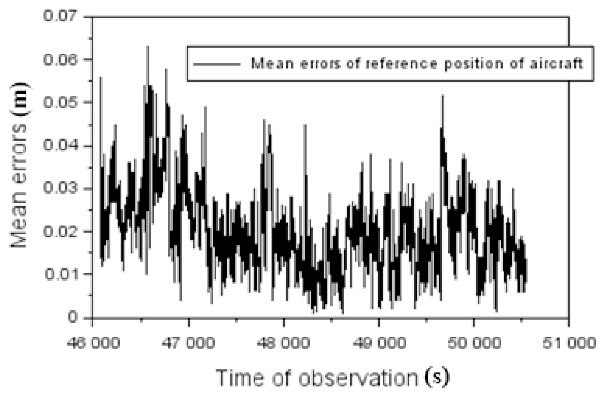
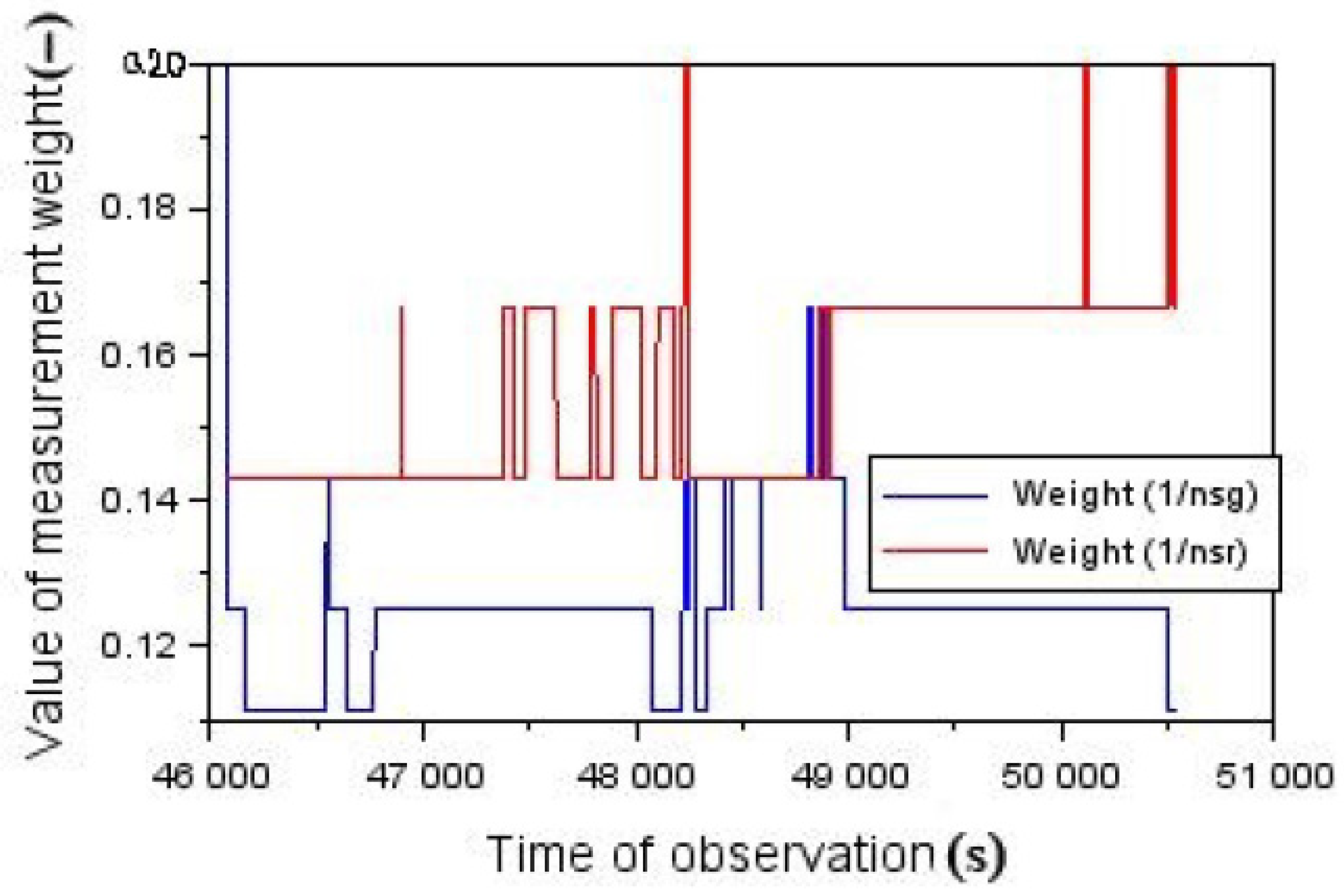
Other model parameters, such as the multipath effect, tidal and geodynamic corrections and phase slip, were used in the calculations.

The second part of the research was carried out in Scilab v.6.0.0 [43] for Equations (4)–(9). In the Scilab program, the Seneca Piper PA34-200T aircraft’s position coordinates were imported from the GPS and GLONASS solutions, and then, the alignment model was set up according to Equation (4). The final calculations in Scilab were performed for mathematical Equations (4)–(9). Calculations in Scilab were performed for all readings of the aircraft position from the GPS and GLONASS solutions. The reference position of the aircraft was calculated using the RTK-OTF solution in Trimble Total Control v.2.700 software.

Numerical calculations in the CSRS-PPP software, Scilab software and Trimble Total Control program were performed post-factum after a flight test of a Seneca Piper PA34-200T aircraft.

For the purposes of scientific research in aviation, the state of the ionosphere was determined by the VTEC (Vertical TEC) parameter. The VTEC value was determined based on the GIM (Global Ionosphere Maps) ionosphere model from the CODE (Center for Orbit Determination in Europe) Analysis Center in Switzerland [44]. The VTEC parameter fluctuated during the flight tests from 16.8 TECU to 17.3 TECU.

5. Results

The presentation of the research results began with determining the mean reference position errors from the RTK-OTF solution. Figure 2 shows the results of the mean reference flight position errors. The mean errors were resolved as in Equation (6), and these values are the resultant mean errors for the XYZ coordinates. The RTK-OTF solution used precise GPS and GLONASS phase observations at the L1/L2 frequencies. Analyzing the obtained results, the resultant aeroplane position’s mean errors were from 0.005 m to 0.063 m. Over 52% of the mean error results were less than 0.02 m. In turn, over 84% of the results of the mean error were less than 0.03 m.

In the next step, the measurement weights, i.e., the values of the coefficients $(a,b,c,d,e,f)$ used in Equation (4), are shown. The weighting factors’ values were calculated based on Equation(5). In Figure 3, the values of the coefficients $(a,b,c,d,e,f)$ for measuring the weights $(a=c=e=\frac{1}{n{s}_g}=P_g;b=d=f=\frac{1}{n{s}_r}=P_r)$ are shown. For the solution of the PPP GPS position, the measurement weight was from 0.111 to 0.200. On the other hand, for the PPP GLONASS position solution, the measuring balance results were from 0.143 to 0.200. You can see that the measurement weights were not the same as the numbers of the GPS and GLONASS satellites, which also varied during the experiment.

Moreover, Figure 4 shows the results of the coefficient values $(a,b,c,d,e,f)$ for measuring weights $(a=c=e=\frac{1}{C{l}_g^2}=P_g;b=d=f=\frac{1}{C{l}_r^2}=P_r)$. In this case, the coefficient values $(a=c=e)$ for the GPS PPP solution ranged from 0.012 to 0.037. For the PPP GLONASS solution, the values of the coefficients varied from 0.008 to 0.014.

The next test results concerned the distribution of corrections $(V_{g,x},V_{g,y},V_{g,z},V_{r,x},V_{r,y},V_{r,z})$ for the XYZ components. Figure 5, Figure 6 and Figure 7 show the correction values as a function of the experiment’s duration. The dispersion along the X-axis is from −0.903 m to +0.675 m. When analyzing the dispersion of corrections in the function of measuring weights, it can be noticed that the corrections $V_{g,x}$ range from +0.204 m to +0.675 m. In turn, respectively, the distribution of corrections $V_{r,x}$ from the minimum and maximum values is from −0.903 m to −0.362 m. For the Y component, the spread of corrections is from −2.162 m to +1.644 m. In the case of corrections $V_{g,y}$, their values are from +1.007 m to +1.644 m. For corrections $V_{r,y}$, their values are from −2.162 m. to −0.856 m. The distribution of corrections along the Z-axis is very interesting. When we compare the results of corrections between Figure 5, Figure 6 and Figure 7, we can see at once that the distributions in Figure 7 are an order of magnitude smaller than in Figure 5 and Figure 6. That causes the scatter of the Z coordinate obtained results as the smallest around the expected value. Especially when we look at the distribution of corrections in Figure 7, it can be concluded that their dispersion is from −0.284 m to +0.201 m. It can be seen that we deal with the results that best correspond to the expected values of the Z components. The $V_{g,z}$ corrections distribution is from +0.097 m to +0.201 m and $V_{r,z}$ corrections from −0.284 m to +0.026 m, respectively.

Then, in Figure 8, Figure 9 and Figure 10, the results of the calculated mean errors $({\sigma }_x,{\sigma }_y,{\sigma }_z)$ are presented separately for the resultant XYZ coordinates of the aircraft position. It should be added that the parameter values $({\sigma }_x,{\sigma }_y,{\sigma }_z)$ are shown for two weight models, i.e., $P_g=\frac{1}{n{s}_g}\begin{array}{c}\end{array}\vee \begin{array}{c}\end{array}{P}_g=\frac{1}{C{l}_g^2}$ and $P_r=\frac{1}{n{s}_r}\begin{array}{c}\end{array}\vee \begin{array}{c}\end{array}{P}_r=\frac{1}{C{l}_r^2}$. When observing Figure 8, Figure 9 and Figure 10, it can be seen that, when we use the weight in the inverse of the mean error function, we get better results than when we weight in the joint function of the number of tracked GPS or GLONASS satellites. Therefore, the values ${\sigma }_x$ are from 0.246 m to 0.323 m when using measuring weights $P_g=\frac{1}{n{s}_g}$ and $P_r=\frac{1}{n{s}_r}$. On the other hand, when we use measuring weights $P_g=\frac{1}{C{l}_g^2}$ and $P_r=\frac{1}{C{l}_r^2}$, then the ${\sigma }_x$ values are from 0.071 m to 0.110 m. The ${\sigma }_x$ values were reduced by over 66% when we used weights $(P_g=\frac{1}{C{l}_g^2};P_g=\frac{1}{C{l}_r^2})$ compared to weights $(P_g=\frac{1}{n{s}_g};P_r=\frac{1}{n{s}_r})$ in the calculations. The mean errors ${\sigma }_y$ were from 0.571 m to 0.769 m when using weights $P_g=\frac{1}{n{s}_g}$ and $P_r=\frac{1}{n{s}_r}$. On the other hand, when we used measuring weights $P_g=\frac{1}{C{l}_g^2}$ and $P_r=\frac{1}{C{l}_r^2}$, then the ${\sigma }_y$ values were from 0.183 m to 0.267 m. The ${\sigma }_y$ values were reduced by about 65% when we used weights $(P_g=\frac{1}{C{l}_g^2};P_g=\frac{1}{C{l}_r^2})$ compared to the application of $(P_g=\frac{1}{n{s}_g};P_r=\frac{1}{n{s}_r})$ in the calculations. The mean errors ${\sigma }_z$ had values from 0.001 m to 0.089 m when using weights $P_g=\frac{1}{n{s}_g}$ and $P_r=\frac{1}{n{s}_r}$. When we used measuring weights $P_g=\frac{1}{C{l}_g^2}$ and $P_r=\frac{1}{C{l}_r^2}$, then the ${\sigma }_z$ parameters ranged from 0.001 m to 0.029 m. In this case, it can also be said that the use of measuring weights $(P_g=\frac{1}{C{l}_g^2};P_g=\frac{1}{C{l}_r^2})$ reduced the mean errors ${\sigma }_z$ by over 65% compared to the solution using $(P_g=\frac{1}{n{s}_g};P_r=\frac{1}{n{s}_r})$.

The test results in Figure 11 and Figure 12 show the $(M_x,M_y,M_z)$ parameter values for the solution using measuring weights $(P_g=\frac{1}{n{s}_g};P_r=\frac{1}{n{s}_r})$ and $(P_g=\frac{1}{C{l}_g^2};P_g=\frac{1}{C{l}_r^2})$. The $(M_x,M_y,M_z)$ values for weights $(P_g=\frac{1}{C{l}_g^2};P_g=\frac{1}{C{l}_r^2})$ are up to 0.544 m. In turn, the $(M_x,M_y,M_z)$ values for weights $(P_g=\frac{1}{C{l}_g^2};P_g=\frac{1}{C{l}_r^2})$ are up to 0.189 m. It can be concluded that the $(M_x,M_y,M_z)$ parameters for solving a position using $(P_g=\frac{1}{C{l}_g^2};P_g=\frac{1}{C{l}_r^2})$ improved by about 65% to 66% compared to the corresponding results for these quantities when weights $(P_g=\frac{1}{n{s}_g};P_r=\frac{1}{n{s}_r})$ were used.

Table 1. The results of the global chi-square test.

Coordinate	Measurement Weight	$\mathbf{Maximum} \mathbf{Values} \mathbf{of} {\mathit{\sigma }}_0^2\cdot (\mathit{n}-1),$ $\mathbf{Where}: {\mathit{\sigma }}_0^{}=({\mathit{\sigma }}_{\mathit{x}}^{},{\mathit{\sigma }}_{\mathit{y}}^{},{\mathit{\sigma }}_{\mathit{z}}^{})$	$\mathbf{Statistical} \mathbf{Value} \mathbf{of} {\mathit{\chi }}_{\mathit{f},1-\mathit{\alpha }}^2$
X	$(P_g=\frac{1}{n{s}_g};P_r=\frac{1}{n{s}_r})$	0.323	3.841
Y	$(P_g=\frac{1}{n{s}_g};P_r=\frac{1}{n{s}_r})$	0.769	3.841
Z	$(P_g=\frac{1}{n{s}_g};P_r=\frac{1}{n{s}_r})$	0.089	3.841
X	$(P_g=\frac{1}{C{l}_g^2};P_g=\frac{1}{C{l}_r^2})$	0.110	3.841
Y	$(P_g=\frac{1}{C{l}_g^2};P_g=\frac{1}{C{l}_r^2})$	0.267	3.841
Z	$(P_g=\frac{1}{C{l}_g^2};P_g=\frac{1}{C{l}_r^2})$	0.029	3.841

shows the results of the ${\sigma }_0^2\cdot (n-1)$ chi-square test’s parameters and table values ${\chi }_{f,1-\alpha }^2$ at the $1-\alpha =0.95$ confidence level and for $f=n-1$ degrees of freedom. The parameter results ${\sigma }_0^2\cdot (n-1)$ were smaller than the tabulated ${\chi }_{f,1-\alpha }^2$ values, so the global chi-square statistical test, which determines the internal reliability of the performed alignment, was fulfilled and implemented. In the analyzed case, the tabular value of the chi-square test was 3.841. Value ${\sigma }_0^{}$ denotes parameters $({\sigma }_x^{},{\sigma }_y^{},{\sigma }_z^{})$, respectively. Moreover, the number of degrees of freedom $f=n-1$ is equal to 1. The chi-square test in the analyzed example was carried out and checked for each measurement epoch. The chi-square test was fulfilled for all measurement epochs, making the obtained test results more reliable in the experiment.

The last stage of the research concerned determining the accuracy of the presented research method. In this, Equation (9) from the research methodology was used. The position errors $DX$ were from +0.032 m to +0.527 m for weights $(P_g=\frac{1}{n{s}_g};P_r=\frac{1}{n{s}_r})$. On the other hand, for weights $(P_g=\frac{1}{C{l}_g^2};P_g=\frac{1}{C{l}_r^2})$, the position errors $DX$ were from −0.244 m to +0.206 m. It could be observed that the positioning accuracy along the X-axis improved by about 87% in the case of using weights $(P_g=\frac{1}{C{l}_g^2};P_g=\frac{1}{C{l}_r^2})$ in relation to the results of $DX$ determined for the $(P_g=\frac{1}{n{s}_g};P_r=\frac{1}{n{s}_r})$ weighing process. The $DY$ position errors were from −1.051 m to −0.492 m for $(P_g=\frac{1}{n{s}_g};P_r=\frac{1}{n{s}_r})$ weighing. On the other hand, for $(P_g=\frac{1}{C{l}_g^2};P_g=\frac{1}{C{l}_r^2})$, the $DY$ position errors were −0.433 m to +0.173 m. It can be concluded that the positioning accuracy along the Y-axis improved by over 85% in the case of using $(P_g=\frac{1}{C{l}_g^2};P_g=\frac{1}{C{l}_r^2})$ in relation to the $DY$ results determined for the $(P_g=\frac{1}{n{s}_g};P_r=\frac{1}{n{s}_r})$. The $DZ$ position errors were from −0.451 m to +0.183 m for weights $(P_g=\frac{1}{n{s}_g};P_r=\frac{1}{n{s}_r})$. In turn, for $(P_g=\frac{1}{C{l}_g^2};P_g=\frac{1}{C{l}_r^2})$, the $DZ$ position errors were −0.396 m to +0.228 m. It is worth noting that the positioning accuracy along the Z-axis improved by more than 11% when weights $(P_g=\frac{1}{C{l}_g^2};P_g=\frac{1}{C{l}_r^2})$ were used in relation to the results determined for weights $(P_g=\frac{1}{n{s}_g};P_r=\frac{1}{n{s}_r})$ (Please see Figure 13, Figure 14 and Figure 15).

6. Discussion

In the discussion of the results, the attention is mainly focused on determining the proposed test method’s external reliability. For this purpose, the proposed algorithm was verified in terms of determining positioning accuracy. In the discussion, the aircraft position’s obtained results using the PPP method from the RTKLIB program [45,46] for the weighted average model used were analyzed. Such a check is crucial, because we obtain independent confirmation of the proposed mathematical algorithm’s correctness (4–9). In particular, in the proposed research method’s external control, the key factor is Equation (9), thanks to which, the position errors can be determined [47]. Therefore, the weighted average model results will be compared to the reference coordinates determined by RTK-OTF. Figure 16, Figure 17 and Figure 18 show the positioning accuracy between the weighted average model and the RTK technique as a function of the measurements used. The $DX$ position errors were from +0.157 m to +1.668 m for weights $(P_g=\frac{1}{n{s}_g};P_r=\frac{1}{n{s}_r})$. On the other hand, for $(P_g=\frac{1}{C{l}_g^2};P_g=\frac{1}{C{l}_r^2})$, the $DX$ position errors were from −0.077 m to +0.883 m. It can be observed that the positioning accuracy along the X-axis improved by about 45% in the case of using weights $(P_g=\frac{1}{C{l}_g^2};P_g=\frac{1}{C{l}_r^2})$ in relation to the $DX$ results determined when weights $(P_g=\frac{1}{n{s}_g};P_r=\frac{1}{n{s}_r})$ were used.

The $DY$ position errors were from −0.745 m to +0.812 m for $(P_g=\frac{1}{n{s}_g};P_r=\frac{1}{n{s}_r})$ weighing. In turn, for $(P_g=\frac{1}{C{l}_g^2};P_g=\frac{1}{C{l}_r^2})$, the $DY$ position errors were from −0.081 m to +0.754 m. It can be observed that the positioning accuracy along the Y-axis improved by about 82% in the case of using $(P_g=\frac{1}{C{l}_g^2};P_g=\frac{1}{C{l}_r^2})$ in relation to the $DY$ results determined for weights $(P_g=\frac{1}{n{s}_g};P_r=\frac{1}{n{s}_r})$.

The $DZ$ position errors ranged from −2.021 m to −0.228 m for $(P_g=\frac{1}{n{s}_g};P_r=\frac{1}{n{s}_r})$. On the other hand, for $(P_g=\frac{1}{C{l}_g^2};P_g=\frac{1}{C{l}_r^2})$ weighing, the position errors were −1.604 m to +0.295 m. It is worth noting that the positioning accuracy along the Z-axis improved by over 59% when $(P_g=\frac{1}{C{l}_g^2};P_g=\frac{1}{C{l}_r^2})$ weighting was used in relation to the $DZ$ results determined for the $(P_g=\frac{1}{n{s}_g};P_r=\frac{1}{n{s}_r})$ weighing process.

The aircraft positioning results obtained during the research using the PPP method for the GPS and GLONASS solutions showed the high quality and accuracy of the moving object’s determined coordinates. The presented research method significantly improved the accuracy of PPP GPS and PPP GLONASS positioning in relation to the RTK solution. The obtained research results showed that the applied computational scheme of the mathematical model fits well in the modern trend of scientific research on the application of the PPP method in air navigation, as in other works [6,7,8,9,10,11,12,13,14,15,16,17,18,19,20,21,22,23,24,25,26,27,28,29,30,31,32,33,34]. That is important, because the developed computational algorithm improved the performance of position determination and, at the same time, the accuracy of PPP positioning, as in works [6,7,8,9,10,11,12,13,14,15,16,17,18,19,20,21,22,23,24,25,26,27,28,29,30,31,32,33,34]. It should be mentioned that the research problem of improving the performance of the PPP method in air navigation is a current and extremely interesting topic; hence, there have been a large number of research papers [6,7,8,9,10,11,12,13,14,15,16,17,18,19,20,21,22,23,24,25,26,27,28,29,30,31,32,33,34] undertaken by scientists worldwide. The topic should be constantly developed in the aviation industry, especially in Poland, which needs modern solutions in implementing GNSS systems in aviation. The use of PPP measurement technology in the positioning of aircrafts can accelerate research on the determination of the quality of GNSS satellite positioning in aviation, especially the positioning accuracy parameter. The submitted research work shows that modern navigation solutions in Polish aviation are needed and require implementation.

7. Conclusions

The paper presented the results of research on the application of a new research method for improving the performance of computing aircraft coordinates from GPS and GLONASS solutions for the PPP measurement technique. The paper addressed the problem of improving GPS and GLONASS positioning accuracy in the PPP method by developing a new computational algorithm based on a linear combination of individual GNSS solutions, i.e., GPS and GLONASS. The algorithm used a weighted mean model between the XYZ geocentric coordinates from the GPS and GLONASS. The mathematical relationship was based on the determination of six linear coefficients $(a,b,c,d,e,f)$, which linked the XYZ position coordinate readings together. The whole computational scheme was solved by the weighted mean model, taking into account different measurement weights. The measurement weights were a function of the number of GPS and GLONASS satellites and, also, as the inverse of the square of the mean error. Moreover, the whole algorithm was tested on GPS and GLONASS kinematic data from an airborne experiment carried out with a Seneca Piper PA34-200T aircraft at the Mielec airport. A dual-frequency dual-system GPS/GLONASS receiver was placed on-board the aircraft, which made it possible to record the GNSS observations, which were then used to calculate the aircraft’s position in CSRS-PPP software. The calculated XYZ position coordinates from the CSRS-PPP software were used in the developed optimization algorithm and implemented in the Scilab programming language. The accuracy of the presented research method was checked and verified with the results obtained from the RTK-OTF solution. Moreover, the proposed solution’s accuracy was better by 11–87% for the model with the weighting scheme as a function of the inverse of the square of the mean error. The performance of the algorithm was also tested for results from another navigation software, i.e., RTKLIB. In this case, the algorithm’s accuracy for the improvement of PPP positioning was better by 45–82% for the model with the weighting scheme as a function of the inverse of the square of the mean error. The presented method’s effectiveness was relatively high and could be used to improve the performance of GPS and GLONASS in PPP positioning method for air navigation.

References

1. International Civil Aviation Organization. ICAO Standards and Recommended Practices (SARPS), Annex 10, Volume 1 (Radio Navigation Aids). 2006. Available online: https://www.ulc.gov.pl/pl/prawo/prawomi%C4%99dzynarodowe/206-konwencje (accessed on 15 January 2021).
2. Krasuski, K. Application the GPS Code Observations in BSSD Method for Recovery the Position of the Aircraft. J. Autom. Mob. Robot. Intell. Syst 2017, 11, 45–52. [Google Scholar] [CrossRef]
3. Krasuski, K. Utilization CSRS-PPP software for recovery aircraft’s position. Sci. J. Sil. Univ. Technol. Ser. Transp. 2015, 89, 61–68. [Google Scholar] [CrossRef]
4. Grzegorzewski, M.; Jaruszewski, W.; Fellner, A.; Oszczak, S.; Wasilewski, A.; Rzepecka, Z.; Kapcia, J.; Poplawski, T. Preliminary results of DGPS/DGLONASS aircraft positioning in flight approaches and landings. Annu. Navig. 1999, 1, 41–53. [Google Scholar]
5. Grzegorzewski, M. Navigating an aircraft by means of a position potential in three dimensional space. Annu. Navig. 2005, 9, 111. [Google Scholar]
6. El-Mowafy, A. Precise Point Positioning in the airborne mode. Artif. Satell. 2011, 46, 33–45. [Google Scholar] [CrossRef] [Green Version]
7. Abdel-tawwab Abdel-salam, M. Precise Point Positioning Using Undifferenced Code and Carrier Phase Observations. Ph.D. Thesis, University of Calgary, Calgary, AB, Canada, September 2005. [Google Scholar]
8. Gao, Y.; Chen, K. Performance Analysis of Precise Point Positioning using real-time orbit and clock products. J. Glob. Position. Syst. 2004, 3, 95–100. [Google Scholar] [CrossRef]
9. Gao, Y.; Wojciechowski, A. High precision kinematic positioning using single dual frequency GPS receiver. Int. Arch. Photogramm. Remote Sens. Spat. Inf. Sci. 2004, 34, 845–850. [Google Scholar]
10. Shimizu, Y.; Murata, M. Flight Evaluation of GPS Precise Point Positioning Software for Helicopter Navigation. SICE J. Control Meas. Syst. Integr. 2008, 1, 362–367. [Google Scholar] [CrossRef]
11. Gross, J.N.; Watson, R.M.; D’Urso, S.; Gu, Y. Flight-Test Evaluation of Kinematic Precise Point Positioning of Small UAVs. Int. J. Aerosp. Eng. 2016, 1259893. [Google Scholar] [CrossRef] [Green Version]
12. Hutton, J.J.; Gopaul, N.; Zhang, X.; Wang, J.; Menon, V.; Rieck, D.; Kipka, A.; Pastor, F. Centimeter-Level Robust Gnss-Aided Inertial Post-Processing for Mobile Mapping Without Local Reference Stations. In Proceedings of the International Archives of the Photogrammetry, Remote Sensing and Spatial Information Sciences, XXIII ISPRS Congress, Prague, Czech Republic, 12–19 July 2016; Volume XLI-B3, pp. 819–826. [Google Scholar] [CrossRef] [Green Version]
13. Zhang, X. Precise Point Positioning: Evaluation and Airborne Lidar Calibration; Danish National Space Center: Copenhagen, Denmark, 2006.
14. Waypoint Products Group. Airborne Precise Point Positioning (PPP) in GrafNav 7.80 with Comparisons to Canadian Spatial Reference System (CSRS) Solutions; NovAtel Inc.: Calgary, AB, Canada, 2006; 8p. [Google Scholar]
15. Chen, K.; Gao, Y. Real-Time Precise Point Positioning Using Single Frequency Data. In Proceedings of the 18th International Technical Meeting of the Satellite Division of The Institute of Navigation (ION GNSS 2005), Long Beach, CA, USA, 13–16 September 2005; pp. 1514–1523. [Google Scholar]
16. Le, A.Q.; Tiberius, C. Single-frequency precise point positioning with optimal filtering. GPS Solut. 2007, 11, 61–69. [Google Scholar] [CrossRef] [Green Version]
17. Grayson, B.; Penna, N.T.; Mills, J.P.; Grant, D.S. GPS precise point positioning for UAV photogrammetry. Photogramm. Rec. 2018, 33, 427–447. [Google Scholar] [CrossRef] [Green Version]
18. Yuan, X.; Fu, J.; Sun, H.; Toth, C. The application of GPS precise point positioning technology in aerial triangulation. ISPRS J. Photogramm. Remote Sens. 2009, 64, 541–550. [Google Scholar] [CrossRef]
19. Gao, Z.; Zhang, H.; Ge, M.; Niu, X.; Shen, W.; Wickert, J.; Schuh, H. Tightly coupled integration of ionosphere-constrained precise point positioning and inertial navigation systems. Sensors 2015, 15, 5783–5802. [Google Scholar] [CrossRef] [Green Version]
20. Gao, Z.; Shen, W.; Zhang, H.; Niu, X.; Ge, M. Real-time Kinematic Positioning of INS Tightly Aided Multi-GNSS Ionospheric Constrained PPP. Sci. Rep. 2016, 6, 30488. [Google Scholar] [CrossRef] [Green Version]
21. Kjørsvik, N.S.; Gjevestad, J.G.O.; Brøste, E.; Gade, K.; Hagen, O.-K. Tightly coupled precise point positioning and inertial navigation systems. In Proceedings of the International Calibration and Orientation Workshop EuroCOW 2010, Castelldefels, Spain, 10–12 February 2010. [Google Scholar]
22. Roesler, G.; Martell, H. Tightly coupled processing of Precise Point Position (PPP) and INS data. In Proceedings of the 22nd International Meeting of the Satellite Division of the Institute of Navigation, Savannah, GA, USA, 22–25 September 2009; pp. 1898–1905. [Google Scholar]
23. Shi, J.; Yuan, X.; Cai, Y.; Wang, G. GPS real-time precise point positioning for aerial triangulation. GPS Solut. 2017, 21, 405–414. [Google Scholar] [CrossRef]
24. Krasuski, K.; Wierzbicki, D.; Jafernik, H. Utilization PPP method in aircraft positioning in post-processing mode. Aircr. Eng. Aerosp. Tech. 2018, 90, 202–209. [Google Scholar] [CrossRef]
25. Grzegorzewski, M.; Ciećko, A.; Oszczak, S.; Popielarczyk, D. Autonomous and EGNOS Positioning Accuracy Determination of Cessna Aircraft on the Edge of EGNOS Coverage. In Proceedings of the 2008 National Technical Meeting of The Institute of Navigation, San Diego, CA, USA, 28–30 January 2008; pp. 407–410. [Google Scholar]
26. Ćwiklak, J.; Kozuba, J.; Krasuski, K.; Jafernik, H. The assessment of aircraft positioning accuracy using GPS data in RTK-OTF technique. In Proceedings of the 18th International Multidisciplinary Scientific GeoConference SGEM 2018, Sofia, Bulgaria, 2–8 July 2018; pp. 459–466, ISBN 978-619-7408-40-9. [Google Scholar] [CrossRef]
27. Krasuski, K.; Kobialka, E.; Grzegorzewski, M. Research of Accuracy of the Aircraft Position Using the GPS and EGNOS Systems in Air Transport. Commun. Sci. Lett. Univ. Zilina 2019, 21, 27–34. [Google Scholar] [CrossRef]
28. Ćwiklak, J.; Kozuba, J.; Krasuski, K.; Jafernik, H. Determination of the aircraft position in PPP method in an in-flight test—Case study. In Proceedings of the 18th International Multidisciplinary Scientific GeoConference SGEM 2018, Sofia, Bulgaria, 2–8 July 2018; pp. 133–140, ISBN 978-619-7408-40-9. [Google Scholar] [CrossRef]
29. Kozuba, J.; Krasuski, K. Utilization of the PPP method for precise positioning of the aircraft in air navigation. In Proceedings of the 22nd International Scientific Conference Transport Means 2018, Trakai, Lithuania, 3–5 October 2018; pp. 16–21. [Google Scholar]
30. Krasuski, K. Aircraft positioning using SPP method in GPS system. Aircr. Eng. Aerosp. Tech. 2018, 90, 1213–1220. [Google Scholar] [CrossRef]
31. Krasuski, K. Application the Single Difference Technique in Aircraft Positioning Using the GLONASS System in the Air Transport. Commun. Sci. Lett. Univ. Zilina 2019, 21, 51–58. [Google Scholar] [CrossRef]
32. Krasuski, K.; Jafernik, H. Applied GLONASS observations in PPP method in airborne test in Mielec. Inform. Autom. Pomiary Gospod. Ochr. Śr. 2016, 6, 83–88. [Google Scholar] [CrossRef]
33. Jafernik, H.; Krasuski, K.; Cwiklak, J. Application the PPP Method in aircraft positioning in air navigation. Revist. Eur. Derecho Navega. Marít. Aeronáut. 2017, 34, 1–10. [Google Scholar]
34. Krasuski, K.; Cwiklak, J.; Jafernik, H. Aircraft positioning using PPP method in GLONASS system. Aircr. Eng. Aerosp. Tech. 2018, 90, 1413–1420. [Google Scholar] [CrossRef]
35. Krasuski, K.; Ciećko, A.; Bakuła, M.; Wierzbicki, D. New Strategy for Improving the Accuracy of Aircraft Positioning Based on GPS SPP Solution. Sensors 2020, 20, 4921. [Google Scholar] [CrossRef] [PubMed]
36. Monico, J.F.G.; Marques, H.A.; Tsuchya, I.; Oyama, R.T.; Queiroz, W.R.S.; Souza, M.C.; Wentz, J.P. Real Time PPP Applied to Airplane Fligtht Tests. Bull. Geod. Sci. 2019, 25, e2019007. [Google Scholar] [CrossRef] [Green Version]
37. Navipedia Website. Available online: https://gssc.esa.int/navipedia/index.php/Receiver_Antenna_Phase_Centre (accessed on 30 October 2020).
38. Hadaś, T. GNSS-WARP software for real-time Precise Point Positioning. Artif. Satell. 2015, 50, 59–76. [Google Scholar] [CrossRef] [Green Version]
39. Leandro, R.; Santos, M.; Langley, R. Analyzing GNSS data in precise point positioning software. GPS Solut. 2011, 15, 1–13. [Google Scholar] [CrossRef]
40. Krasuski, K. The impact of IGS precise products in aircraft positioning in air navigation. Pomiary Autom. Robot. 2018, 2, 61–66. [Google Scholar] [CrossRef]
41. Osada, E. Geodesy; Oficyna Wydawnicza Politechniki Wrocławskiej: Wroclaw, Poland, 2001; ISBN 83-7085-663-2. [Google Scholar]
42. CSRS-PPP Tools Website. Available online: https://webapp.geod.nrcan.gc.ca/geod/tools-outils/ppp.php (accessed on 30 October 2020).
43. Scilab Website. Available online: https://www.scilab.org/ (accessed on 30 October 2020).
44. CODE LAC Website. Available online: http://ftp.aiub.unibe.ch/CODE/ (accessed on 30 October 2020).
45. Takasu, T. RTKLIB ver. 2.4.2 Manual, RTKLIB: An Open Source Program. Package for GNSS Positioning. 2013. Available online: http://www.rtklib.com/prog/manual_2.4.2.pdf (accessed on 30 October 2020).
46. Abdel-Maguid, R.H. Assessment and Testing of GPS kinematic Surveys using Precise Point Positioning Technique. J. Eng. Comput. Sci. 2016, 8, 81–94. [Google Scholar]
47. Specht, M. Consistency of the Empirical Distributions of Navigation Positioning System Errors with Theoretical Distributions—Comparative Analysis of the DGPS and EGNOS Systems in the Years 2006 and 2014. Sensors 2021, 21, 31. [Google Scholar] [CrossRef] [PubMed]
Figure 1. The aircraft trajectory in-flight experiment in Mielec airport [own material].
Energies 14 02525 g001
Figure 2. Mean errors of aircraft position from the RTK-OTF solution.
Energies 14 02525 g002
Figure 3. Values of the weights ( a = c = e = 1 n s g = P g ; b = d = f = 1 n s r = P r ) for the adjustment scheme.
Energies 14 02525 g003
Figure 4. Value of the weights ( a = c = e = 1 C l g 2 = P g ; b = d = f = 1 C l r 2 = P r ) for the adjustment scheme.
Energies 14 02525 g004
Figure 5. Residuals ( V g , x ; V r , x ) along the X-axis.
Energies 14 02525 g005
Figure 6. Residuals ( V g , y ; V r , y ) along the Y-axis.
Energies 14 02525 g006
Figure 7. Residuals ( V g , z ; V r , z ) along the Z-axis.
Energies 14 02525 g007
Figure 8. Mean errors σ x along the X-axis.
Energies 14 02525 g008
Figure 9. Mean errors σ y along the Y-axis.
Energies 14 02525 g009
Figure 10. Mean errors σ z along the Z-axis.
Energies 14 02525 g010
Figure 11. Mean errors of the arithmetic means ( M x , M y , M z ) from the adjustment scheme ( P g = 1 n s g ; P r = 1 n s r ) .
Energies 14 02525 g011
Figure 12. Mean errors of the arithmetic means ( M x , M y , M z ) from the adjustment scheme ( P g = 1 C l g 2 ; P g = 1 C l r 2 ) .
Energies 14 02525 g012
Figure 13. Position errors along the X-axis.
Energies 14 02525 g013
Figure 14. Position errors along the Y-axis.
Energies 14 02525 g014
Figure 15. Position errors along the Z-axis.
Energies 14 02525 g015
Figure 16. Position errors along the X-axis.
Energies 14 02525 g016
Figure 17. Position errors along the Y-axis.
Energies 14 02525 g017
Figure 18. Position errors along the Z-axis.
Energies 14 02525 g018