1. Introduction
With climate change issues becoming more pressing recently, the interest in research dedicated to mitigating the consequences through energy efficiency improvements has increased. Therefore, various research projects suggesting different ways of tackling the problem have emerged, aiming to help Europe reach the established energy targets. Within the European goals to cut greenhouse gas emissions by 20%, produce 20% of energy from renewables, and improve energy efficiency by 20% [
1], the EU Horizon 2020 Fostering Energy Efficiency and BehAvioural Change through Information and Communication Technology (ICT) (FEEdBACk) project specifically aims to aid in achievement of the latter objective by increasing energy efficiency through behavioral change using ICT solutions. Particularly, it aims to bridge two knowledge fields that have traditionally been apart from each other: social sciences and engineering. As was recently demonstrated in [
2], the occupants’ behavior significantly influences the building’s energy efficiency, while the motivation for energy savings varies across occupants, due to the split incentive problem [
3]. Thus, specific strategies, such as eco-feedback, social interaction, and gamification [
4,
5] have to be implemented to promote behavioral change towards more energy-responsible attitudes. The FEEdBACk project deploys various gamification techniques supported by the advanced algorithmic landscape and extensive metering and sensing infrastructure, making it stand out from the cohort of similar projects [
6,
7,
8]. While the idea, methodology, contribution, and main results of the FEEdBACk project are well detailed in respective papers [
9], this work aims to demonstrate the real-world implementation and functionality of the developed ICT-based platform, suitable for different types of tertiary and residential buildings. In the context of the current study, the platform’s operations are showcased on an office building and multiple residential dwellings. The platform is composed of various interconnected software applications that, together, are used to provide intelligent building services, thus assisting facility managers in their decision-making process and delivering optimization solutions for improved building operation and maintenance. Moreover, the usage of various forecasting techniques allows the platform to efficiently anticipate future operations, thus determining the best guidelines for planning ahead. Although most of the advanced engineering algorithms that compose the core of the platform have been presented and detailed earlier in the literature [
10,
11,
12], the platform’s integrated nature was not showcased elsewhere. Therefore, in this paper, we present the ICT-based platform’s operational results, obtained during the testing phase, and assess their quality. Although evaluating the performance of the ICT-based platform as a whole would be preferable, envisaging a single metric that could summarize this is difficult. Thus, each application’s results are discussed with respect to specific metrics deemed applicable to the underlying methodologies.
The remainder of this paper is structured as follows:
Section 2 describes the demonstration sites within the FEEdBACk project involved in the testing phase of the ICT-based platform.
Section 3 presents the ecosystem of applications deployed in the FEEdBACk project and elaborates on their purpose and functionality within the ICT-based platform.
Section 4 demonstrates the operations of the ICT-based platform, discusses particular results achieved by individual applications during the testing phase, and reflects on the performance of the ICT-based platform and its usability in the real-world.
Section 5 concludes the paper.
2. Demonstration Sites
The current paper showcases the ICT-based platform’s operational results, obtained at two demonstration sites participating in the FEEdBACk project: Porto and Lippe.
The Porto demo site located in Portugal with its oceanic climate is represented by the INESC TEC headquarters consisting of two contiguous building sections, A and B, built in different years but similar in both their internal and external structure. The combined building covers a usable area of 4000 m2 with a daily occupancy of about 400 users. Although the facilities are open 24/7, most of the users work between 9 a.m. and 7 p.m. on weekdays. The building’s Heating, Ventilation, and Air Conditioning (HVAC) system is composed of two parts: a central unit that facilitates the heating/cooling of the water circulating throughout the building and a ventilation system comprised of fans present in each rooms. For space heating, a gas boiler is used, which heats the water to 80 °C and keeps the temperature constant regardless of demand. For cooling, a compression system with an ice bank is utilized, where the latter generates the ice overnight to provide cooling functionalities for the day ahead. A set of 68 solar panels distributed over six strings, each with its own solar inverter, is located on the building’s rooftop, amounting to the total power of 14.6 kW. These panels are oriented to the South and, due to their location and disposition of the surrounding buildings, they have an excellent sun exposure without any kind of shadows, regardless the time of year. The buildings do not possess any energy storage.
The Lippe demo site is located in the village of Dörentrup in Germany and consists of about 30–40 private residential dwellings. Dörentrup is a part of the maritime-structure of North-West Germany, with an average altitude of 130 m. The winter is under the influence of the Atlantic, the summer is mostly moderately warm, and the rainfall is relatively equal over the months. The households do not differ substantially in either the occupied area or the description of underlying individual energy systems. Most of them are one- to two-floor residences which were mainly built more than 20 years ago. However, they have been recently renovated, which makes them very modern and efficient. Some of the houses are equipped with solar thermal energy or photovoltaic systems in which excess production is sent to the electricity grid. The households are predominantly heated with gas or oil, which is mainly dedicated to hot water production. About half of the households have another heating system based on wood-fire ovens. Usually, the buildings are not equipped with any ventilation; thus, this is done naturally using the window opening.
3. Ecosystem of Applications
In the FEEdBACk project, we developed a set of tools with the ultimate goal of aiding interested building stakeholders in understanding where the greatest energy costs reside, how to optimize “when and at which rate” energy should be buffered and consumed, and the best practices to improve their energy efficiency.
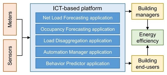
Figure 1 represents the way these tools interact with each other. Overall, they can be divided into four large groups:
External Inputs;
DEXCell;
Applications;
Gamification Platform.
External inputs can be grouped into three categories: smart meters that measure energy consumption, sensors that provide information about temperature, humidity, illuminance, and CO2 concentration, thus describing the overall quality of the environment, and finally, questionnaires that help us to segment ICT platform’s users depending on their level of ecological awareness.
DEXCell [
13], a platform provided by one of the FEEdBACk’s partners, encompasses data storage capabilities with Graphical User Interface (GUI), referred to as FEEdBACk Suite. Thus, most of the data related to the project are saved into DEXCell and visualized through GUI. This platform is more focused on building managers or owners.
The applications developed in the project, due to their specificity, are running on partners’ servers. However, all generated inputs and outputs are stored in DEXCell. The following applications are presented in this paper, with their details provided in the consecutive subsection:
Net Load Forecast application;
Occupancy Forecast application;
Load Disaggregation application;
Automation Manager application;
Behavior Predictor application.
The gamification platform consists of a set of elements that aim to provide the user, through a mobile application, an experience that leads to encouraging more efficient energy utilization and more responsible consumer behaviour. It acts as the interface between the ICT platform and the end-user, who coincides with the owner in the case of residential households. This platform aims to increase users’ engagement through interactive and competitive games and raise awareness about their energy-related behavior. Moreover, throughout the platform, users receive personalized notifications, according to the profile attributed to them using the questionnaire, and indications of energy-saving opportunities. These interactions allow users to compare themselves with their opponents in the game and understand if they are saving more or less energy, thereby increasing visibility, awareness, and commitment. Some specific strategies to improve users’ learning and understanding of energy efficiency include rewarding schemes [
14] and extensive usage of various learning objects, such as videos and quizzes, that are available weekly according to the defined learning and engagement plan.
An interested reader can find more details about each of the four groups encompassing the tools developed in the FEEdBACk project in [
9].
The applications developed using Python programming language are based on open-source libraries and run in an exclusive virtual machine operating on the Ubuntu server. The DEXCell platform uses a cloud system that automatically adapts the storage needs according to the number of simultaneous users. The gamification platform relies on a PHP web service that secures the transfer of information between the databases (DBs) and the mobile application, available in both Android and iOS. The information generated by applications, such as the gamification platform, is stored in a MySQL DB, while the information exchange between different platform’s components is supported by the REST Application Programming Interface (API).
The information stored on the platform’s DBs, which results from either data inputs or the outputs generated by the applications, amounts to 1 GB per year. The tools themselves occupy around 2 GB, where approximately 90% of that storage capacity is dedicated to the baseline creation.
3.1. Applications
As in
Section 4, we aim to demonstrate the results produced by developed applications: this section briefly introduces each of them, particularly focusing on their purpose, while the underlying methodologies are discussed in respective sections.
3.1.1. Net Load Forecast
The net load represents the balance of electrical energy consumption at the building level, defined as the difference between electrical energy demand and onsite electrical power generation from photovoltaic panels. Thus, the Net Load Forecast application aims to forecast such net load for the following day. The Net Load Forecast can be exploited in several ways, such as by being used in an optimization algorithm to maximize building’s energy self-consumption or shared with an aggregator of prosumers that participates in energy and reserves markets [
15]. In the particular context of FEEdBACk, it should be noted that, since each of the INESC TEC buildings described in
Section 2 has several smart meters installed, it is possible to measure energy consumption at a sub-building level (e.g., just the lights or HVAC), which, in turn, allows for forecasting consumption for sub-building level, thus facilitating data exploitation by the Behaviour Predictor (
Section 4.5), Load Disaggregation (
Section 4.3), and Automation Manager (
Section 4.4) applications.
3.1.2. Occupancy Forecast
This application generates buildings’ occupancy forecasts for the day ahead. Particular occupancy predictions can be attributed either to a building as a whole or to specific zones or rooms within the building. The obvious advantage of implementing this tool is that it allows the building’s management team to plan how controllable equipment, such as HVAC, should be operated. Moreover, the application helps identify energy-saving situations that do not alter the users’ comfort, such as turning off the lights in an unoccupied room.
3.1.3. Load Disagregation
Load Disaggregation application aims to provide an overview of the electricity consumption in buildings. For instance, it transforms the whole-building aggregated power measurements to specific consumption values allocated to devices’ categories. The application allows the physical monitoring of individual appliances’ power consumption to be avoided, employing a non-intrusive load-monitoring technique. Therefore, such an approach not only contributes to preserving occupants’ privacy but also saves the effort and cost of sensor installation at each power outlet in the building. Moreover, it applies to both tertiary and residential buildings.
3.1.4. Automation Manager
One of the most energy-consuming systems in a large building is the HVAC system. This system consists of central equipment that produces both heat and cold, and in certain cases, does this simultaneously. To optimize HVAC equipment’s energy consumption, taking into account future needs, the Automation Manager application was developed. This app produces day-ahead ON/OFF operational profiles of HVAC, taking exogenous variables, such as external temperature, day of the week, expected occupancy, etc, into account. If the equipment does not allow remote automation, it will be up to the building manager to program the necessary needs. However, when automation possibility exists, the system can remotely switch the HVAC equipment ON and OFF.
3.1.5. Behaviour Predictor
The Behaviour Predictor’s main purpose is to identify opportunities that lead to a reduction in electrical energy consumption and a change in behavior towards the more rational use of that energy. Analyzing the estimated consumption, this application can detect specific periods with excessive consumption and send alerts to users, giving advice on lowering their energy consumption. This advice is not intended to interfere with users’ comfort. An example of such advice would be: “Aren’t you sure about what you can do for the environment? We have detected an opportunity that will help you: there is a moderate temperature outdoors (less than 26 °C). Why don’t you turn off the air conditioner and open the windows instead?”
The following section elaborates on the methodologies underlying the applications and presents the results obtained through each of them during extensive testing on real-world data. Notably, the datasets used to assess the applications’ performance were collected at the FEEdBACk project’s demonstration sites described in
Section 2, while the training and testing periods were chosen as the trade-off between data availability, volume, and quality.
4. Results
4.1. Net Load Forecast
Net Load Forecast is based on two independent applications: Load Forecast and Photovoltaic (PV) Forecast, each with their own approach. The forecasts are generated daily at midnight, requiring a training step beforehand, which is also performed daily. For the PV Forecast, the training is done using Gradient Boosting Trees Regression [
12]. In contrast, the Load Forecast uses an approach comprising an ensemble of Naïve, Gradient Boosting Trees [
16], Conditional Kernel Density Estimation [
17], and a model based on data from the previous week. The Naïve model assumes the load of the previous working day for working days, and for weekends, it assumes the load is equal to the corresponding previous weekend day. The model based on data from the previous week’s uses the load from the previous seven days as input, along with calendar variables. The ensemble approach consists of computing each model’s prediction followed by selecting the top two performing models based on a prediction error calculated on the most recent month.
Although the algorithms were designed to produce forecasts for up to 48 h ahead, in this paper, we utilize the day-ahead window to account for the needs and interactions between the applications in FEEdBACk.
Table 1 presents the training and testing periods of the Net Load Forecast application. The training set is a moving window comprising a previous year in the Load Forecast and two years in the PV Forecast case.
In
Table 2 and
Table 3, the inputs and outputs of the two applications are detailed: both use historical data to train the models, namely, weather data and power metering, alongside calendar variables. In real-time, the algorithms use forecasts of weather variables generated by the mesoscale Weather Research and Forecasting model, currently available at [
18]. The temperature and relative humidity refer to values in the building exterior and their forecasted values are calculated on the weather station’s side. The input power metering data corresponds to 185 smart meters installed at INESC TEC and can be divided into the following categories: lights, outlets, HVAC, fan, splitter, hand dryer, lifts, server room, and server HVAC [
9]. In some cases, we use these data to monitor a single room’s load; otherwise, we aggregate it at the building level. Although smart meters collect data every 15 min (average power), PV generation measurements were obtained at hourly resolution from respective inverters (average power). As an output, we produce load forecasts for each smart meter, while PV generation is forecasted as a whole.
This section aims to provide the results of the Net Load Forecast in two steps. First, we analyze the net load of INESC TEC at the building level. Second, we investigate the disaggregated load forecast at room level, namely, the open space located at INESC TEC building B, as described in
Section 2. In the second part of the analysis, we address the following variables, which are used as input in the Behaviour Predictor application (
Section 4.5): outlets, lights, and HVAC fans. To evaluate the performance of the Net Load Forecast application we use the normalized Mean Absolute Error (nMAE) and normalized Root Mean Square Error (nRMSE) metrics defined in Equations (
1) and (
2), respectively.
where each
is the forecasted value,
is the observed value,
n is the number of observations, and
is the normalizing factor equal to the maximum observed value. One should note that error metrics were not computed for the net load, as it corresponds to the difference between the two generated forecasts. In
Table 4 the average power values produced by the forecasts were transformed into energy values to provide a meaningful comparison between the two forecasts: it can be concluded that, aggregating the entire testing period results, the PV forecast has a larger error than the load forecast. The former is overestimated, while the latter is underestimated.
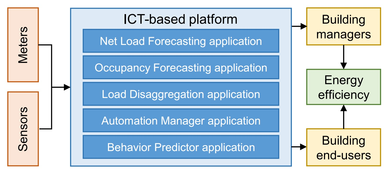
Figure 2 presents one week of Net Load Forecast compared with the ground truth.
Table 5 presents the results of Load Forecast per load type obtained in room B2.2 for the duration of the whole testing period. To assess the quality of obtained forecasts, we developed a Naïve model, as previously described. Summarizing the results presented in
Table 5, we conclude that the ensemble load forecast reasonably improves the Naïve forecast. At the same time, we notice that the ensemble load forecast slightly underestimates the total load values in all cases. To demonstrate another phenomenon that happens on the weekends, we show one typical week of the test set in
Figure 3. Particularly, one can see that weekends (days 11 and 12) pose a problem for both Naïve and ensemble models because such a load is simply very difficult to predict during non-working days in the office.
4.2. Occupancy Forecast
There are two types of algorithm developed for occupancy forecasting in the framework of the FEEdBACk project, with their methodology, design, validation, and testing detailed extensively in [
11]. The first algorithm belongs to the supervised machine learning category and deploys a support-vector machine to forecast occupancy from labeled low-frequency power data. The raw smart meter measurements are transformed using feature engineering into three feature categories: statistical, load curve shape, and time-related. More details on the manual feature extraction procedure can be found in [
11]. The second algorithm is unsupervised and uses a long short-term memory neural network with additional regressors such as holidays, weekends, and time of day to predict occupancy from ambient environment measurements obtained through the multi-sensor solution. The sensors’ data flows are fused using the trust layer-enabled majority voting procedure explained in [
11].
This section aims to showcase the operation of both algorithms comprising the Occupancy Forecasting application on the selected testing period stated in
Table 6. The training period, equally indicated in
Table 6, is used by the supervised algorithm to effectively train historical labeled data effectively.
To evaluate the performance of the Occupancy Forecasting application, we utilize the accuracy metric detailed in Equation (
3); as in the presence of ground truth, the occupancy prediction task can be framed as a classification problem:
In the present case study, the supervised occupancy forecasting algorithm is deployed at the whole-building level, while the unsupervised one is deployed at the room level. The following subsections present the results obtained through the Occupancy Forecasting application on the test dataset.
4.2.1. Supervised Occupancy Forecasting
Table 7 elaborates on the inputs and outputs of the supervised occupancy forecasting algorithm. As such a method requires training, historical information on occupancy and building load curves is collected with 15-min resolution. The prior is obtained using a clock-card method that records the number of building users at entrances. The latter is extracted using a conventional smart meter. An interested reader can find more details on the data collection process in [
9]. Along with historical data, the forecast values of power load, obtained from the Net Load Forecasting application described in
Section 4.1, are required to generate the occupancy output. In binary logic, 0 signifies absence, and 1 means presence.
Figure 4 depicts the supervised occupancy forecasting algorithm results on the selected part of the test dataset. One can notice that the algorithm’s presence and absence predictions are generally well synchronized with the ground truth. However, if the power values drop to their minimum, some misclassifications of occupancy occur. This phenomenon is particularly noticeable in October. The overall accuracy achieved by the supervised occupancy forecasting algorithm on the full test dataset is 94.7%.
4.2.2. Unsupervised Occupancy Forecasting
Table 8 declares the inputs and outputs of the unsupervised occupancy forecasting algorithm. The main inputs contain the historical measurements of temperature, relative humidity, illuminance, and equivalent CO
2 concentration obtained with 15-min resolution using the multi-sensor solution developed in the FEEdBACk project [
9]. The latter is based on the measurements of total volatile organic compounds and aims to approximate the real CO
2 concentration levels. In this case study, a single multi-sensor is used to collect necessary data as it can sufficiently cover the office space.
Figure 5 depicts the results obtained with the unsupervised occupancy forecasting algorithm along with the inputs to the Occupancy Forecasting application. Although it was not possible to collect the ground truth from the considered office space, several observations can be made based on the obtained results. First, the office appears to have less regular occupancy patterns, although the presence periods are aligned with the whole-building occupancy forecast. Second, humidity and temperature seem to have more influence on predicted occupancy, while the impact of illuminance is less obvious. Moreover, the multi-sensor location was potentially not ideal, as the equivalent CO
2 concentration measurements do not fluctuate. Possibly, the sensor was in a well-ventilated place where it could have been influenced by door and window opening, or it was located too distantly from the office user, so the equivalent CO
2 concentration did not build up. A previous study of forecasting occupancy using the unsupervised approach in conjunction with multi-sensor data demonstrated 97.6% of accuracy [
11].
4.3. Load Disaggregation
The Load Disaggregation application is based on two disaggregation algorithms: one is suitable for tertiary buildings, while the other is applicable to residential dwellings. The tertiary algorithm is supervised and utilizes training on historical data to disaggregate smart meter measurements into HVAC, light, and other categories. The two main machine-learning models deployed are XGBoost and Random forest regression. The residential disaggregation algorithm resorts to Markov models to infer eight distinct categories of domestic appliances. Particularly, for each person in the household, the algorithm generates an activity chain based on the probability of various activities with time, such as cooking, cleaning, eating, showering, etc. Afterwards, each activity is matched with a set of domestic appliances, each belonging to the specific disaggregation category, that could have been used during this activity. The quality of the devices’ assignment is determined by the error between the measured aggregated load curve and the cumulative load curve, obtained as the sum of allocated devices’ nominal powers. Further details about the methodology, design, and implementation of the residential disaggregation algorithm called Device Usage Estimation (DUE) algorithm is described in detail in [
10].
This section aims to provide the Load Disaggregation application results on the test dataset indicated in
Table 9. The training dataset is utilized by the tertiary algorithm, while the residential algorithm does not require training.
To evaluate the performance of the Load Disaggregation application, the following metrics indicated in Equations (
4) and (
5) are utilized:
where
and
are the predicted and the ground truth power of category
m at time
t. To calculate the difference between the two Energy Shares, the Energy Share Error metric explained in Equation (
6) is used:
The reasons for choosing the metrics related to Energy Share per category are detailed in [
10].
4.3.1. Tertiary Load Disaggregation
Table 10 summarizes the tertiary part of the Load Disaggregation application’s inputs and outputs. The main inputs include hourly aggregated and sub-metered energy consumption, which the algorithm transforms from its raw form to additionally include standby, mean, and total daily energy consumption. Other inputs include cooling-degree and heating-degree days obtained from [
19] as well as time-related features, namely day of the week, month, and day of the year. The outputs contain daily energy consumption shares of HVAC and light, together with the other category, which agglomerates various appliances outside the first two categories. Notably, beyond the training data acquired from the building of interest itself, the tertiary load disaggregation algorithm is additionally pre-trained on the measurements collected from similar buildings present in one of the FEEdBACk partner’s commercial database. Thus, some of the discrepancies between the obtained results and the building’s ground truth can be explained by such additional pre-training procedures.
Figure 6 depicts the results of the tertiary Load Disaggregation application on the test dataset. The Energy Share of HVAC consumption is overestimated, resulting in underestimation of the Energy Share dedicated to light. However, for both categories, the respective Energy Share Error
does not exceed 15%, which can be considered satisfactory, as it is in line with previously demonstrated results through state-of-the-art disaggregation algorithms [
10].
To provide a more thorough analysis of the results, we calculated the daily average Energy Shares per category and divided them into weekday and weekend values. As shown in
Table 11, the disaggregation algorithm catches the overall tendency of reduced energy consumption for HVAC during weekends compared to weekdays. However, the achieved values differ from the ground truth, which is related to the overestimation of the HVAC category. For the light, the algorithm predicts rather constant energy consumption throughout the week, although the ground truth shows that the share of light decreases during the weekend.
4.3.2. Residential Load Disaggregation
Table 12 describes the inputs and outputs of the residential part of the Load Disaggregation application. The unsupervised DUE algorithm utilizes the building’s load curves, collected using a conventional smart meter as the main input. Additionally, the information related to the household’s characteristics, such as the number of occupants, their age and their employment status, is collected through the survey. More details on the inputs of the residential load disaggregation algorithm can be found in [
10]. The outputs contain load curves disaggregated to eight different categories: cooking, standby, housekeeping, fridge, entertainment, ICT, heating, and lighting. Although the algorithm can provide specific load curves for each category at a 15-min resolution, its main purpose is to estimate the respective energy consumption shares. Therefore, in the course of the FEEdBACk project, the Energy Share per category
is used and displayed to household’s inhabitants.
Table 13 presents the results of the Load Disaggregation application on 10 selected households from the German demonstration site of the FEEdBACk project, as described in
Section 2. As detailed, the sub-metering of household appliances is not available at this demonstration site; the disaggregation results are compared to the statistics of electrical energy usage in German private households, depicted in
Figure 7.
Several observations can be made to summarize the results obtained. First, the Energy Share of the heating category is largely underestimated due to the existing limitation of the DUE algorithm’s current implementation. Particularly, the current DUE implementation considers only the hairdryer in the heating category, thus omitting other potential heating devices, such as heat pumps. Second, fridge and standby consumption is overestimated, while the Energy Shares of ICT, housekeeping, and entertainment are underestimated. The results of the cooking and light categories fall in the ballpark of statistical values, as their standard deviation from the statistics does not exceed 5% and equals to 3.3% and 2.2%, for cooking and light, respectively. However, one should keep in mind that statistics used for comparison date back to 2006; thus, they might not correspond to the modern energy consumption tendencies due to domestic appliances’ technological progress. Regardless, the obtained average Energy Share Errors per category do not exceed 20%, which is in line with DUE’s performance evaluated through an extensive benchmarking procedure against other state-of-the-art disaggregation methods, presented in [
10].
4.4. Automation Manager
The core of the Automation Manager application is the occupancy-centric rule-based HVAC automation algorithm, the methodology and design of which are detailed in [
11]. The algorithm aims to provide near-optimal day-ahead ON/OFF schedules for heating and cooling systems present in the building.
Table 14 summarizes the inputs and outputs of the Automation Manager application. All inputs can be divided into three categories: static, historical, and forecast. The static inputs include the building area and heating and cooling cut-off temperatures determined based on EN15251 regulation. The cut-off temperatures’ constant values were chosen to ensure the general thermal comfort of the occupants, as accounting for each individual’s comfort conditions is not possible due to variations in occupants’ metabolism rate, type of clothing, age, gender, and other personal characteristics. The historical inputs contain past values of the building’s heating demand, outdoor temperature, solar irradiance, and occupancy. The algorithm requires such historical variables to calculate the building’s heat transfer coefficients needed to calculate the thermal load. The detailed procedure of estimating these coefficients using the Newton–Raphson method is described in [
11]. The forecast variables include outdoor temperature, solar irradiance, and occupancy. While the prior two are obtained using the weather service presented in
Section 4.5, the latter constitutes the output of the Occupancy Forecasting app described in
Section 4.2. As all forecast variables except binary occupancy are retrieved with an hourly resolution, the occupancy is downsampled. The outputs of the Automation Manager application are obtained in the form of heating and cooling ON/OFF schedules with hourly resolution.
The HVAC automation algorithm functions according to the set of rules extensively described in [
9]. In this paper, we provide a shortened version of the rules’ description to help the reader further understand the results:
If the building’s thermal load is positive, the heating should be turned on. If it is negative, the cooling is on;
If the outdoor temperature is lower or equal to the heating cut-off temperature, the heating is on. If it is higher than or equal to the cooling cut-off temperature, the cooling is on;
If there is at least one occupant present in a space, heating or cooling might be turned on. If the space is empty, both systems are turned off to avoid energy waste;
No simultaneous operation of heating and cooling systems is allowed;
If the outdoor temperature fluctuations are short-term and not significant in their order of magnitude, no intermediary on/off switch should be realized. Instead, the guidelines should be kept similar to the ones of the previous time window.
To evaluate the performance of the Automation Manager application, the near-optimal or so-called improved HVAC simulated schedules are compared with the conventional time-scheduling method. The underlying logic is that improved heating and cooling schedules result in potential energy savings as they rely on occupancy forecasts and thus have a better knowledge of when either heating or cooling are actually needed in the building. The potential energy savings are calculated according to Equation (
7):
where
N is the number of the time intervals in the period of interest,
is the HVAC power consumption at time interval
. Conventional
and improved
HVAC schedule indicators represent whether the HVAC system should be turned ON or OFF at each particular time interval.
The Automation Manager case study is conducted within the training and testing periods indicated in
Table 15. The training period is required to estimate the heat transfer coefficients described previously. The testing period is the period during which we are interested in obtaining improved HVAC schedules. In the current study, the HVAC automation is applied only to working days, Monday to Friday. Additionally, the conventional time-based ON/OFF schedule is assumed to activate HVAC according to typical heating and cooling seasons in Portugal. Thus, heating is turned on from November to April, while the cooling is switched on from May to October. During each working day, the conventional schedule operates between 8 a.m. and 7 p.m.
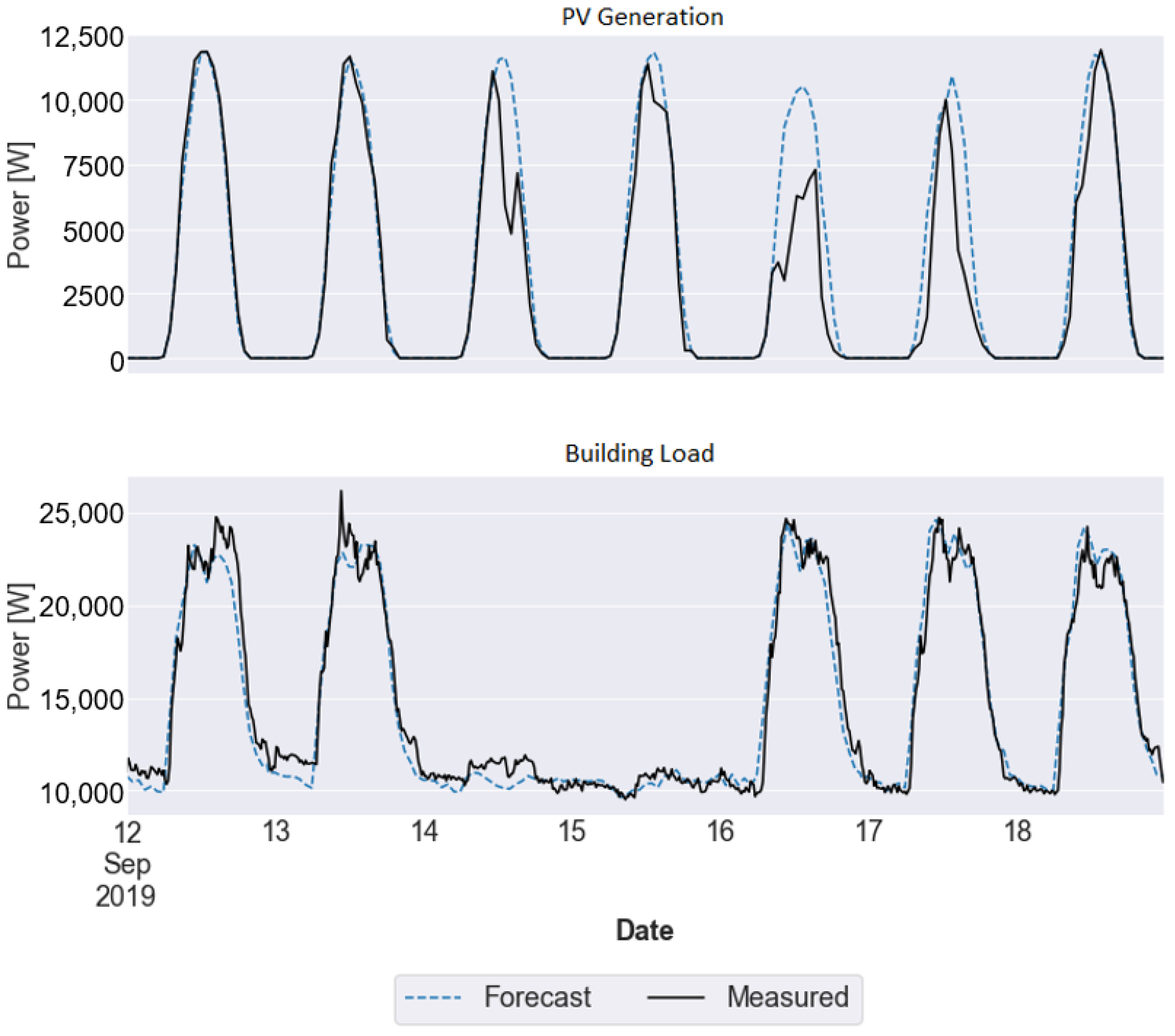
Figure 8 depicts the results obtained through the Automation Manager on the test dataset. The overall quantity of potential energy savings obtained during the testing period amounted to 25.3%. Within this value, 89.8% were achieved during the cooling season, while only 10.2% during the heating season. The underlying reasons are threefold. First, during the cooling period, the temperature values were more frequently located in the dead-band, which is the temperature range between the heating cut-off and the cooling cut-off. Therefore, the HVAC was not activated in these circumstances. Second, the heat gains from solar radiation were more substantial in summer and early autumn. Last, during the cooling season, the occupancy rate was inferior to the heating season, as the building’s users spent more time outdoors. Therefore, the HVAC was not switched on when the absence was forecasted.
4.5. Behaviour Predictor
The Behaviour Predictor application resorts to machine learning techniques to predict opportunities for lowering energy consumption. The original intention of the Behavior Predictor can be summarized in three main steps. First, at midnight, the algorithm detects hours of excessive energy consumption based on the day-ahead forecasts. Here, “excessive” is determined for each particular case by analyzing the historical data available, e.g., retrieving the median value of energy consumption when the room is empty. Second, it sends a corresponding set of alerts to the Gamification Platform that delivers these messages to building users’ smartphones. Finally, based on metered energy consumption, the impact of delivered messages on energy savings is computed and saved for future reference. The historical data of users’ reaction to notifications sent by the Gamification Platform provides valuable information that can be exploited by targeting only those building users that are forecasted to deliver significant energy savings. However, the original intention of the Behaviour Predictor could not be fully implemented due to COVID-19. Therefore, the implemented version simplifies the former and is presented in
Figure 9. The simplification is that the algorithm does not compute the forecasted energy savings when the Gamification Platform sends messages. Note that the results of Behavior Predictor rely heavily on the outputs of Occupancy Forecast (
Section 4.2) and Net Load Forecast (
Section 4.1) applications.
The Behavior Predictor is composed by five models, which can be resumed as follows:
Plugs empty: occupancy transition hour (room is occupied in hour h and will not be occupied in hour h + 1), while plug consumption is considered high relative to hours when it is unoccupied;
Plugs occupied: room is occupied, while plugs consumption is considered high relative to hours when it is occupied;
Lights: occupancy transition hour (room is occupied in hour h and will not be occupied in hour h + 1), while light consumption is considered high relative to hours when it is unoccupied;
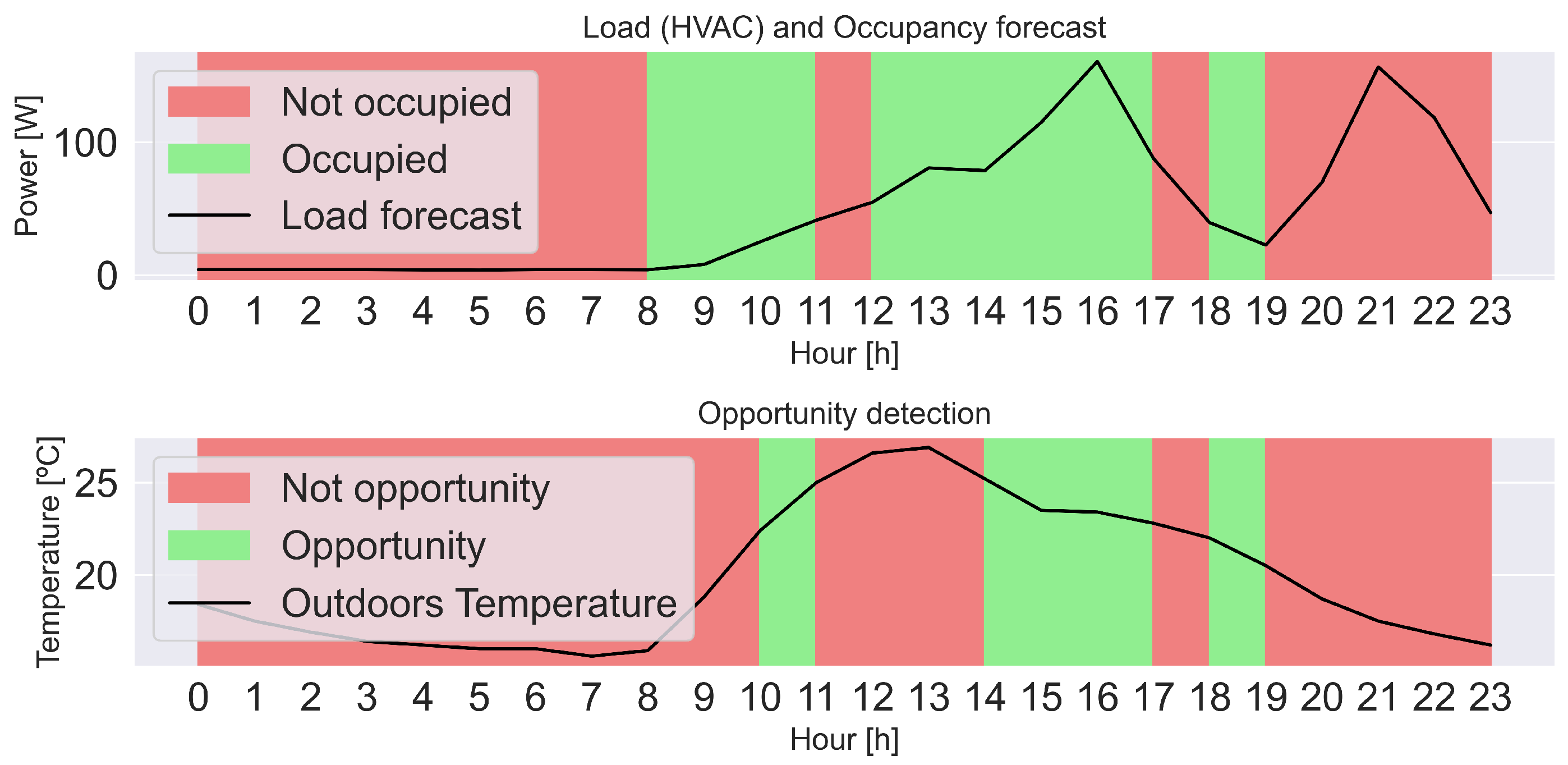
HVAC moderate: room is occupied, while outdoor temperature is moderate (<26 °C in warm months and >20 °C in cold months), while HVAC consumption is predicted to be in use;
HVAC empty: occupancy transition hour (room is occupied in hour h and will not be occupied in hour h + 1), while HVAC consumption is considered high relative to hours when it is unoccupied;
These models run daily at midnight, producing a forecast window for the next 24 h with a time step of 1 h. These forecasts can anticipate opportunities for lowering energy consumption and can be used, for example, to send notifications to building users, as envisioned by the FEEdBACk’s Gamification Platform. The output is binary; thus, each hour is either an opportunity or a non-opportunity. For this reason, in our methodology, we considered it a binary classification problem and implemented decision trees using scikit-learn [
21]. For further details about the implementation of the Behavior Predictor module, an interested reader may consult [
9].
Table 16 summarizes the inputs and outputs of the Behavior Predictor app.
The models are trained with the historical energy consumption of plugs, lights, and HVAC, obtained from smart meters. To produce results, the Behavior Predictor app uses forecasts of average power consumption produced by the Net Load Forecast app (
Section 4.1), which are obtained with 15-min resolution and transformed into hourly resolution. Moreover, we use two calendar variables: the working day variable helps avoid sending messages to the Gamification Platform that would trigger notifications to users who are not in the building. The winter variable is used to differentiate cold months (October to March) from warm months (April to September) in the HVAC moderate model. In the training phase, the threshold for acceptable use of HVAC depends on the outdoor temperature: warmer than 20 °C in cold months and cooler than 26 °C in warm months. The Occupancy Forecast app produces binary results using the unsupervised algorithm (
Section 4.2), readily used by the Behavior Predictor at the room level. As Behavior Predictor works with an hourly resolution, while the Occupancy Forecast has a time step of 15 min, we assume that when a room is occupied for at least 15 min, the room is considered occupied during that hour. The occupancy transition is a detection for the hour when the room is empty after being occupied in the previous hour. The outdoor temperature forecast [
22] is used with no further adjustments.
Table 17 presents the dates of training and testing periods, which do not overlap. The training period includes approximately 418 days and 10,000 time-stamped datapoints, while the testing period includes approximately 211 days and 5100 time-stamped data points.
The results of opportunity detection by the Behavior Predictor are summarized in
Table 18. Taking into account that working days constitute approximately 5 of each 7 days in the 211 test days (150 days), each alarm is triggered, on average, from once every working day (HVAC moderate model) to once every two working days (plugs occupied and HVAC empty models).
Some representative results are presented below. Because the Behavior Predictor app operates at the room level, the unsupervised Occupancy Forecasting algorithm is used (
Section 4.2). Thus, no ground truth values are presented.
As can be seen in
Figure 10, occupancy transition hours (i.e., room not occupied in hour
h + 1 and occupied in hour
h) are, in this case, detected as opportunities because the forecasted load, particularly plug consumption, is regarded by the algorithm as high for a non-occupancy hour. Note that, due to utilization of the unsupervised Occupancy Forecasting algorithm, the inputs provided by Occupancy Forecast and Net Load Forecast applications are independent. Thus, a high load forecast does not imply that the room is expected to be occupied (e.g., hours 11–12). This is because unsupervised Occupancy Forecast relies on sensors, not meters, whereas the Net Load Forecast app makes forecasts based on meters. This independence between the two inputs is necessary for the Behavior Predictor. If the Net Load Forecast app and Occupancy Forecast app were using the same inputs, no detection of the unoccupied room during low consumption hours would be possible.
Figure 11 presents the detected opportunities when the room is occupied with high HVAC consumption, while the temperature is moderate. Note that, in hours 13 and 14, the room is forecasted as occupied with high HVAC consumption, but outdoor temperature exceeds the threshold for a warm day. Therefore, the use of HVAC is justifiable and not regarded as an opportunity to lower HVAC consumption. This is in line with the FEEdBACk’s project objective of ensuring the comfort of building users.
5. Conclusions
In this paper, we demonstrated the real-world operation of the ICT-based platform developed in the FEEdBACk project. Particularly, we focused on five main tools, namely, Net Load Forecast, Occupancy Forecast, Load Forecast, Automation Manager, and Behavior Predictor, that compose the ecosystem of applications at the core of the ICT platform. First, using a great level of detail, we presented the inputs and outputs of each application alongside showing their interconnections. Second, we demonstrated the application results obtained during an extensive seven-month testing period in the real-world demonstration sites of the FEEdBACk project. Lastly, we evaluated the performance of applications according to specific metrics rendered suitable for underlying methodologies. As such, we showed that:
The Net Load Forecast application produced PV forecasts within 10% range of measured generation, and aggregated building load forecasts within 4.2% range of measured consumption;
The Occupancy Forecast application, consisting of a supervised and unsupervised algorithms to predict binary occupancy, achieved 94.7% classification accuracy at predicting occupancy in a supervised manner from low-frequency electrical consumption data and showed satisfactory results when using multi-sensor measurements as input to the unsupervised algorithm;
The Load Disaggregation application demonstrated average Energy Share Errors per disaggregation category within 20% range for both supervised and unsupervised methods applied to tertiary Portuguese and residential German data, respectively;
The Automation Manager application generated near-optimal HVAC operational schedules that provided 25.3% of potential energy savings, most of which came from reducing energy spent on cooling;
The Behavior Predictor application, relying on both Net Load Forecast and Occupancy Forecast applications, identified several energy-saving opportunities related to electricity consumption of plugs, lights, and HVAC. Although the results cannot be validated due to the absence of occupancy ground truth, the provided outputs of this application are satisfactory in identifying hours of high consumption related to occupancy in the room.
To conclude, despite the difficulty of imagining a single metric that summarizes the performance of the ICT-based platform as a whole, we showcased its operational viability through a multitude of algorithm-specific metrics. As a result, we not only demonstrated that the ICT-based platform developed in the FEEdBACk project is capable of functioning with real-world data, we confirmed that its application leads to significant improvements in building energy efficiency, achieved through the identification of energy-saving opportunities and intelligent management of controllable devices. Moreover, some of the developed applications, such as Load Disaggregation and Occupancy Forecasting, are suitable for standalone utilization, thus providing functionalities beyond energy efficiency that are relevant for the growing field of household energy management solutions. In addition, the ICT-based platform’s modular structure represents a valuable feature for both research and industry, as it can serve as a base for future complementary software developments, allowing great flexibility, fast prototyping and implementation, and high levels of personalization.
However, the future proliferation of such an ICT-based platform may face certain challenges related to the slow pace of smart metering rollout, long adoption times, and the cost of setup and maintenance prevailing over potential energy savings. To mitigate such foreseeable obstacles, future work should focus on standardizing platform’s specifications, thus turning it into an easily deployable solution and reducing associated costs.
Author Contributions
Conceptualization, F.S., M.D., N.W.; Methodology, M.D., F.R., J.V., N.W.; Software, M.D., F.R., J.V.; Validation, M.D., F.S., N.W.; Formal analysis, M.D., F.R., J.V.; Writing—Original Draft Preparation, M.D., F.R., A.B., J.V.; Writing—Review and Editing, M.D., FS, NW; Visualization, M.D., F.R., A.B., J.V.; Supervision, F.S., N.W.; Project Administration, F.S., N.W.; Funding Acquisition, F.S., N.W. All authors have read and agreed to the published version of the manuscript.
Funding
This project has received funding from the European Research Council (ERC) under the European Union’s Horizon 2020 research and innovation programme (grant agreement n° 768935).
Institutional Review Board Statement
Not applicable.
Informed Consent Statement
Not applicable.
Data Availability Statement
Data available on request due to restrictions. The data presented in this study are available on request from the corresponding author. The data are not publicly available due to use of personal data and the fact that project is still ongoing.
Conflicts of Interest
The authors declare no conflict of interest.
Abbreviations
The following abbreviations are used in this manuscript:
| DUE | Device Usage Estimation |
| GUI | Graphical User Interface |
| HVAC | Heating, Ventilation, and Air Conditioning |
| ICT | Information and Communication Technology |
| PV | Photovoltaic |
References
- European Commission. 2020 Climate & Energy Package. 2021. Available online: https://ec.europa.eu/clima/policies/strategies/2020_en (accessed on 3 March 2021).
- Paone, A.; Jean-Philippe, B. The Impact of Building Occupant Behavior on Energy Efficiency and Methods to Influence It: A Review of the State of the Art. Energies 2018, 11, 953. [Google Scholar] [CrossRef]
- Gillingham, K.; Harding, M.; Rapson, D. Split incentives in residential energy consumption. Energy J. 2012, 33, 1–41. [Google Scholar] [CrossRef]
- Zehir, M.; Ortac, K.; Gul, H.; Batman, A.; Aydin, Z.; Portela, J.; Soares, F.; Bagriyanik, M.; Kucuk, U.; Ozdemir, A. Development and Field Demonstration of a Gamified Residential Demand Management Platform Compatible with Smart Meters and Building Automation Systems. Energies 2019, 12, 913. [Google Scholar] [CrossRef]
- Reeves, B.; Cummings, J.J.; Scarborough, J.K.; Yeykelis, L. Increasing Energy Efficiency with Entertainment Media: An Experimental and Field Test of the Influence of a Social Game on Performance of Energy Behaviors. Environ. Behav. 2015, 47, 102–115. [Google Scholar] [CrossRef]
- UtilitEE. The UtilitEE Project. 2021. Available online: https://www.utilitee.eu/ (accessed on 15 February 2021).
- inBETWEEN. The inBETWEEN Project. 2021. Available online: https://cordis.europa.eu/project/id/768776 (accessed on 15 February 2021).
- eTEACHER. The eTEACHER Project. 2021. Available online: http://www.eteacher-project.eu/ (accessed on 15 February 2021).
- Soares, F.; Madureira, A.; Pagès, A.; Barbosa, A.; Coelho, A.; Cassola, F.; Ribeiro, F.; Viana, J.; Andrade, J.; Dorokhova, M.; et al. FEEdBACk: An ICT-Based Platform to Increase Energy Efficiency through Buildings’ Consumer Engagement. Energies 2021, 14, 1524. [Google Scholar] [CrossRef]
- Holweger, J.; Dorokhova, M.; Bloch, L.; Ballif, C.; Wyrsch, N. Unsupervised algorithm for disaggregating low-sampling-rate electricity consumption of households. Sustain. Energy Grids Netw. 2019, 19, 1–23. [Google Scholar] [CrossRef]
- Dorokhova, M.; Ballif, C.; Wyrsch, N. Rule-based scheduling of air conditioning using occupancy forecasting. Energy AI 2020, 2, 100022. [Google Scholar] [CrossRef]
- Andrade, J.R.; Bessa, R.J. Improving Renewable Energy Forecasting with a Grid of Numerical Weather Predictions. IEEE Trans. Sustain. Energy 2017, 8, 1571–1580. [Google Scholar] [CrossRef]
- DEXMA. DEXMA Energy Intelligence Software. 2021. Available online: https://www.dexma.com/ (accessed on 15 April 2021).
- AlSkaif, T.; Lampropoulos, I.; Van Den Broek, M.; Van Sark, W. Gamification-based framework for engagement of residential customers in energy applications. Energy Res. Soc. Sci. 2018, 44, 187–195. [Google Scholar] [CrossRef]
- Iria, J.; Soares, F.; Matos, M. Optimal bidding strategy for an aggregator of prosumers in energy and secondary reserve markets. Appl. Energy 2019, 238, 1361–1372. [Google Scholar] [CrossRef]
- Ke, G.; Meng, Q.; Finley, T.; Wang, T.; Chen, W.; Ma, W.; Ye, Q.; Liu, T. LightGBM: A Highly Efficient Gradient Boosting Decision Tree. Adv. Neural Inf. Process. Syst. 2017, 30, 3146–3154. [Google Scholar]
- Rothfuss, J.; Ferreira, F.; Walther, S.; Ulrich, M. Conditional Density Estimation with Neural Networks: Best Practices and Benchmarks. arXiv 2019, arXiv:1903.00954. [Google Scholar]
- Meteogalicia. Servidor THREDDS de MeteoGalicia. 2021. Available online: https://www.meteogalicia.gal/web/modelos/threddsIndex.action (accessed on 15 February 2021).
- Weatherbit. The High Performance Weather API for All of your Weather Data Needs. 2021. Available online: https://www.weatherbit.io/ (accessed on 12 March 2021).
- Löfken, J.O. Energy Question of the Week: Who Uses the Most Electricity in Germany? 2010. Available online: https://www.dlr.de/blogs/en/home/energy/energy-question-of-the-week-who-uses-the-most-electricity-in-germany.aspx/searchtagid-50644/10184_page-1/ (accessed on 12 March 2021).
- Pedregosa, F.; Varoquaux, G.; Gramfort, A.; Michel, V.; Thirion, B.; Grisel, O.; Blondel, M.; Prettenhofer, P.; Weiss, R.; Dubourg, V.; et al. Scikit-learn: Machine Learning in Python. J. Mach. Learn. Res. 2011, 12, 2825–2830. [Google Scholar]
- Weather-Service. Outdoor Temperature Forecast. 2021. Available online: http://weather-service.enerapp.com (accessed on 15 February 2021).
Figure 1.
The integration block-scheme in FEEdBACk ICT-based platform.
Figure 1.
The integration block-scheme in FEEdBACk ICT-based platform.
Figure 2.
Results of Net Load Forecast and ground truth on the selected part of test dataset (12 to 19 September 2019).
Figure 2.
Results of Net Load Forecast and ground truth on the selected part of test dataset (12 to 19 September 2019).
Figure 3.
Load (ensemble) forecast, naive forecast, and measurements for whole test dataset on open-space B2.2 of INESC TEC (10 to 17 January 2020).
Figure 3.
Load (ensemble) forecast, naive forecast, and measurements for whole test dataset on open-space B2.2 of INESC TEC (10 to 17 January 2020).
Figure 4.
Results of supervised Occupancy Forecasting app on selected part of test dataset.
Figure 4.
Results of supervised Occupancy Forecasting app on selected part of test dataset.
Figure 5.
Results of unsupervised Occupancy Forecasting app on selected part of test dataset.
Figure 5.
Results of unsupervised Occupancy Forecasting app on selected part of test dataset.
Figure 6.
Predicted and ground truth Energy Shares per tertiary disaggregation category on test dataset.
Figure 6.
Predicted and ground truth Energy Shares per tertiary disaggregation category on test dataset.
Figure 7.
Breakdown of electrical energy consumption in Germany’s private households 2006 [
20].
Figure 7.
Breakdown of electrical energy consumption in Germany’s private households 2006 [
20].
Figure 8.
Comparison between conventional and improved ON/OFF schedules of the HVAC system.
Figure 8.
Comparison between conventional and improved ON/OFF schedules of the HVAC system.
Figure 9.
Behaviour Predictor module.
Figure 9.
Behaviour Predictor module.
Figure 10.
Behaviour Predictor plugs empty model opportunity detection on 2019-08-09.
Figure 10.
Behaviour Predictor plugs empty model opportunity detection on 2019-08-09.
Figure 11.
Behaviour Predictor HVAC moderate model opportunity detection on 2019-08-09.
Figure 11.
Behaviour Predictor HVAC moderate model opportunity detection on 2019-08-09.
Table 1.
Training and testing periods for Net Load Forecast application.
Table 1.
Training and testing periods for Net Load Forecast application.
| Application | Training Period | Testing Period |
|---|
| PV Forecast | 2017-08-01–2019-07-31 | 2019-08-01–2020-02-29 |
| Load Forecast | 2018-08-01–2019-07-31 | 2019-08-01–2020-02-29 |
Table 2.
Detailed list of inputs and outputs for Load Forecast in the Net Load Forecast application.
Table 2.
Detailed list of inputs and outputs for Load Forecast in the Net Load Forecast application.
| Variable | Units | Resolution | Type | Method | Source |
|---|
| Inputs |
| Load | W | 15-min | Historical | Measured | Smart meter |
| Temperature | °C | Hourly | Forecast | Calculated | External weather station |
| Relative humidity | % | Hourly | Forecast | Calculated | External weather station |
| Sine of weekday | n/a | 15-min | Calendar | n/a | n/a |
| Sine of hour | n/a | 15-min | Calendar | n/a | n/a |
| Sine of minute | n/a | 15-min | Calendar | n/a | n/a |
| Cosine of weekday | n/a | 15-min | Calendar | n/a | n/a |
| Cosine of hour | n/a | 15-min | Calendar | n/a | n/a |
| Cosine of minute | n/a | 15-min | Calendar | n/a | n/a |
| Outputs |
| Load | W | 15-min | Forecast | Calculated | Net Load Forecast app |
Table 3.
Detailed list of inputs and outputs for PV Forecast in the Net Load Forecast application.
Table 3.
Detailed list of inputs and outputs for PV Forecast in the Net Load Forecast application.
| Variable | Units | Resolution | Type | Method | Source |
|---|
| Inputs |
| Generation | W | Hourly | Historical | Measured | PV module inverter |
| Surface downwelling shortwave flux | W/m2 | Hourly | Forecast | Calculated | External weather station |
| Temperature | K | Hourly | Forecast | Calculated | External weather station |
| Cloud cover at low levels | n/a | Hourly | Forecast | Calculated | External weather station |
| Cloud cover at mid levels | n/a | Hourly | Forecast | Calculated | External weather station |
| Cloud cover at high levels | n/a | Hourly | Forecast | Calculated | External weather station |
| Cloud cover at mid/high levels | n/a | Hourly | Forecast | Calculated | External weather station |
| Month | n/a | Hourly | Calendar | n/a | n/a |
| Sine of hour | n/a | Hourly | Calendar | n/a | n/a |
| Cosine of hour | n/a | Hourly | Calendar | n/a | n/a |
| Outputs |
| Generation | W | Hourly | Forecast | Calculated | Net Load Forecast app |
Table 4.
Energy [MWh] predicted by Net Load Forecast and resulting errors on test dataset.
Table 4.
Energy [MWh] predicted by Net Load Forecast and resulting errors on test dataset.
| Category | Measured | Forecasted | nMAE | nMRSE |
|---|
| PV | 9.56 | 10.06 | 5.67% | 9.10% |
| Load | 67.97 | 67.80 | 2.68% | 4.17% |
| Net load | 58.40 | 57.74 | - | - |
Table 5.
Energy values (kWh) of load (ensemble) forecast, naive forecast, and measurements for whole test dataset on open-space B2.2 of INESC TEC.
Table 5.
Energy values (kWh) of load (ensemble) forecast, naive forecast, and measurements for whole test dataset on open-space B2.2 of INESC TEC.
| Device | Measured | Model | Forecasted | nMAE | nRMSE |
|---|
| Outlets | 939.15 | Naive | 947.18 | 4.99% | 9.00% |
| Ensemble | 906.52 | 4.55% | 8.17% |
| Lights | 646.11 | Naive | 655.51 | 11.26% | 28.66% |
| Ensemble | 624.50 | 10.90% | 24.05% |
| Fan | 25.28 | Naive | 26.55 | 4.31% | 11.17% |
| Ensemble | 20.84 | 3.78% | 9.73% |
| Aggregated | 1610.53 | Naive | 1629.24 | 6.74% | 11.48% |
| Ensemble | 1563.67 | 6.19% | 9.80% |
Table 6.
Training and testing periods for Occupancy Forecasting application.
Table 6.
Training and testing periods for Occupancy Forecasting application.
| Training Period | Testing Period |
|---|
| 2019-01-01–2019-07-31 | 2019-08-01–2020-02-29 |
Table 7.
Detailed list of inputs and outputs for supervised Occupancy Forecasting application.
Table 7.
Detailed list of inputs and outputs for supervised Occupancy Forecasting application.
| Variable | Units | Resolution | Type | Method | Source |
|---|
| Inputs |
| Occupancy | n/a | 15-min | Historical | Measured | Clock-card |
| Power | W | 15-min | Historical | Measured | Smart meter |
| Power | W | 15-min | Forecast | Calculated | Net Load Forecast app |
| Outputs |
| Binary occupancy | n/a | 15-min | Forecast | Calculated | Occupancy Forecast app |
Table 8.
Detailed list of inputs and outputs for unsupervised Occupancy Forecasting application.
Table 8.
Detailed list of inputs and outputs for unsupervised Occupancy Forecasting application.
| Variable | Units | Resolution | Type | Method | Source |
|---|
| Inputs |
| Temperature | °C | 15-min | Historical | Measured | Multi-sensor |
| Relative humidity | % | 15-min | Historical | Measured | Multi-sensor |
| Illuminance | lux | 15-min | Historical | Measured | Multi-sensor |
| Equivalent CO2 concentration | ppm | 15-min | Historical | Measured | Multi-sensor |
| Outputs |
| Occupancy | n/a | 15-min | Forecast | Calculated | Occupancy Forecast app |
Table 9.
Training and testing periods for Load Disaggregation application.
Table 9.
Training and testing periods for Load Disaggregation application.
| Training Period | Testing Period |
|---|
| 2019-01-01–2019-07-31 | 2019-08-01–2020-02-29 |
Table 10.
Detailed list of inputs and outputs for tertiary Load Disaggregation application.
Table 10.
Detailed list of inputs and outputs for tertiary Load Disaggregation application.
| Variable | Units | Resolution | Type | Method | Source |
|---|
| Inputs |
| Energy consumption | kWh | Hourly | Historical | Measured | Smart meter |
| Energy sub-consumption | kWh | Hourly | Historical | Measured | Sub-metering device |
| Cooling-degree days | °C/day | Daily | Historical | Measured | External weather station |
| Heating-degree days | °C/day | Daily | Historical | Measured | External weather station |
| Outputs |
| HVAC consumption | % | Daily | Historical | Calculated | Load Disaggregation app |
| Lighting consumption | % | Daily | Historical | Calculated | Load Disaggregation app |
| Other consumption | % | Daily | Historical | Calculated | Load Disaggregation app |
Table 11.
Daily average Energy Shares [%] per tertiary disaggregation category on test dataset.
Table 11.
Daily average Energy Shares [%] per tertiary disaggregation category on test dataset.
| Category | Predicted | Ground Truth |
|---|
| Weekday | Weekend | Weekday | Weekend |
|---|
| HVAC | 22.3 | 12.8 | 5.8 | 3.3 |
| Light | 19.5 | 19.6 | 29.0 | 13.9 |
| Other | 58.2 | 67.6 | 65.2 | 82.7 |
Table 12.
Detailed list of inputs and outputs for residential Load Disaggregation application.
Table 12.
Detailed list of inputs and outputs for residential Load Disaggregation application.
| Variable | Units | Resolution | Type | Method | Source |
|---|
| Inputs |
| Power | W | 15-min | Historical | Measured | Smart meter |
| Household characteristics | n/a | n/a | Historical | Measured | Survey |
| Outputs |
| Power per category | W | 15-min | Historical | Calculated | Load Disaggregation app |
| Energy share per category | % | Daily | Historical | Calculated | Load Disaggregation app |
Table 13.
Load disaggregation results for German households: predicted Energy Share [%] per category.
Table 13.
Load disaggregation results for German households: predicted Energy Share [%] per category.
| | ID1002 | ID1004 | ID1007 | ID1009 | ID1011 | ID1012 | ID1013 | ID1014 | ID1017 | ID1022 |
|---|
| Cooking | 5.3 | 3.0 | 4.5 | 10.9 | 10.6 | 7.0 | 11.3 | 6.5 | 5.3 | 13.1 |
| Entertainment | 0.7 | 0.9 | 1.7 | 0.7 | 2.0 | 1.7 | 1.4 | 0.9 | 1.7 | 0.7 |
| Fridge | 11.7 | 27.0 | 29.0 | 45.5 | 23.4 | 47.4 | 39.5 | 55.0 | 32.3 | 23.5 |
| Heating | 0.0 | 0.0 | 0.0 | 0.0 | 0.0 | 0.0 | 0.0 | 0.0 | 0.0 | 0.0 |
| Housekeeping | 1.4 | 2.2 | 9.8 | 1.6 | 4.6 | 2.1 | 8.5 | 19.1 | 11.7 | 6.0 |
| ICT | 0.1 | 0.9 | 1.9 | 0.4 | 0.8 | 0.0 | 0.4 | 0.0 | 0.0 | 0.1 |
| Light | 6.2 | 5.8 | 6.9 | 2.5 | 6.2 | 5.8 | 3.9 | 5.1 | 11.1 | 7.7 |
| Standby | 74.6 | 60.2 | 46.2 | 38.4 | 52.4 | 36.1 | 31.1 | 13.4 | 37.9 | 48.9 |
Table 14.
Detailed list of inputs and outputs for Automation Manager application.
Table 14.
Detailed list of inputs and outputs for Automation Manager application.
| Variable | Units | Resolution | Type | Method | Source |
|---|
| Inputs |
| Cut-off heating temperature | °C | n/a | n/a | n/a | EN15251 regulation |
| Cut-off cooling temperature | °C | n/a | n/a | n/a | EN15251 regulation |
| Building area | m2 | n/a | n/a | Measured | Survey |
| Heating demand | kWh | Hourly | Historical | Measured | Sub-metering device |
| Outdoor temperature | °C | Hourly | Historical | Measured | Weather service |
| Outdoor temperature | °C | Hourly | Forecast | Calculated | Weather service |
| Irradiance | W/m2 | Hourly | Historical | Measured | Weather service |
| Irradiance | W/m2 | Hourly | Forecast | Calculated | Weather service |
| Occupancy | n/a | 15-min | Historical | Measured | Clock-card |
| Binary occupancy | n/a | 15-min | Forecast | Calculated | Occupancy Forecast app |
| Outputs |
| Heating ON/OFF | n/a | Hourly | Forecast | Calculated | Automation Manager app |
| Cooling ON/OFF | n/a | Hourly | Forecast | Calculated | Automation Manager app |
Table 15.
Training and testing periods for Automation Manager application.
Table 15.
Training and testing periods for Automation Manager application.
| Training Period | Testing Period |
|---|
| 2018-10-01–2019-03-01 | 2019-08-01–2020-02-29 |
Table 16.
Detailed list of inputs and outputs for Behaviour Predictor application.
Table 16.
Detailed list of inputs and outputs for Behaviour Predictor application.
| Variable | Units | Resolution | Type | Method | Source |
|---|
| Inputs |
| Power | W | 15-min | Historical | Measured | Smart meter |
| Power | W | 15-min | Forecast | Calculated | Net Load Forecast app |
| Working day | n/a | Daily | Calendar | n/a | n/a |
| Winter | n/a | Daily | Calendar | n/a | - |
| Occupancy forecast (OF) | n/a | 15-min | Forecast | Calculated | Occupancy Forecast app |
| Occupancy transition | n/a | Hourly | Forecast | Calculated | Occupancy Forecast app |
| Outdoors Temperature Forecast | °C | Hourly | Forecast | Calculated | Weather station |
| Outputs |
| Opportunity | n/a | hour | Forecast | Calculated | Behaviour Predictor app |
Table 17.
Training and testing periods for Behaviour Predictor application.
Table 17.
Training and testing periods for Behaviour Predictor application.
| Training Period | Testing Period |
|---|
| 2018-05-25–2019-07-17 | 2019-08-01–2020-02-29 |
Table 18.
Detected opportunities by Behaviour Predictor in 211 test days.
Table 18.
Detected opportunities by Behaviour Predictor in 211 test days.
| Model | Number of Detected Opportunities |
|---|
| Plugs empty | 112 |
| Plugs occupied | 69 |
| Lights | 96 |
| HVAC moderate | 132 |
| HVAC empty | 69 |
| Publisher’s Note: MDPI stays neutral with regard to jurisdictional claims in published maps and institutional affiliations. |
© 2021 by the authors. Licensee MDPI, Basel, Switzerland. This article is an open access article distributed under the terms and conditions of the Creative Commons Attribution (CC BY) license (https://creativecommons.org/licenses/by/4.0/).


 ,
, 


