Sensitivity-Informed Bayesian Inference for Home PLC Network Models with Unknown Parameters

Abstract

Bayesian inference is used to calibrate a bottom-up home PLC network model with unknown loads and wires at frequencies up to 30 MHz. A network topology with over 50 parameters is calibrated using global sensitivity analysis and transitional Markov Chain Monte Carlo (TMCMC). The sensitivity-informed Bayesian inference computes Sobol indices for each network parameter and applies TMCMC to calibrate the most sensitive parameters for a given network topology. A greedy random search with TMCMC is used to refine the discrete random variables of the network. This results in a model that can accurately compute the transfer function despite noisy training data and a high dimensional parameter space. The model is able to infer some parameters of the network used to produce the training data, and accurately computes the transfer function under extrapolative scenarios.

1. Introduction

Power Line Communications (PLC) are expected to be a key component of smart-grids, allowing grid usage to be monitored without adding extensive infrastructure. PLC systems use existing power lines as two-way communication channels and can be implemented in a broad range of scenarios, including home/office networks, device-specific billing, smart energy management, automatic meter reading, and power outage detection [1,2,3,4,5,6]. PLC systems are classified into three categories based on bandwidth: ultra narrowband (UNB) systems have frequencies ranging from 0.3–3 kHz, narrowband (NB) systems have a frequency range of 3–500 kHz, and broadband (BB) systems have frequencies of 1.8–250 MHz [7]. Lower frequencies are less affected by transmission losses and are therefore more effective over long distances, but have a lower data transmission rate. Devices for remote meter reading and monitoring power grid conditions generally use UNB or NB systems. In contrast, BB systems target applications within a home network such as home automation and control, energy management systems, and decreasing energy consumption and cost [8]. The issue with PLC systems is that because they use existing power lines that are not designed for carrying communication signals, and can have high variability in the loads and wiring, the conditions are highly dependent on the specific network topology and loads. Therefore, PLC systems have to be tweaked for specific environments based on the network frequencies, noise, electromagnetic compatibility, and power source. It is important to develop models that can characterize transmission pathways for specific networks to be able to effectively and reliably transmit communications.

There are two existing methods of modeling transmission pathways: top-down and bottom-up models [9,10]. The top-down modeling approach views conductive propagation as an unknown function to be estimated based on training data, and so does not use any prior information such as the network topology or component connections, but rather implements a parametric model based on transmission line (TL) theory [11]. This model, best suited for when the network topology is unavailable, was first proposed by Philips [12], later augmented by Zimmerman and Dostert [13], and it is based on the superposition of signal reflections at various loads predicted by TL theory. The primary disadvantage of a top-down model is that it cannot predict the impact of topology on the conductive propagation pathway, nor how this pathway varies given a change in this topology.

In contrast to a top-down model, bottom-up modeling views conductive propagation as a deterministic quantity of the network topology and its network components. Assuming knowledge of the power network, the network elements can be modeled mathematically to compute the conductive pathway characteristics [14]. Voltage ratios, ABCD matrices, and s-parameters are three popular methods [15] to rigorously incorporate TL theory into models for signal propagation. The bottom-up approach is closely related to the physics of power networks, being derived from electromagnetic wave propagation in transmission line networks, and so can be used for network-related system modeling. On the other hand, the bottom-up approach is computationally complex, and it cannot account directly for unknown network components [14]. There have been many bottom-up network models for different applications and of varying complexity [9,10,16,17,18,19,20]. A recent review of contributions to PLC modeling is provided by Masood et al. [7].

This work combines elements of both top-down and bottom-up modeling to create models with the same framework as bottom-up models, but which use network-specific data to estimate parameters as in top-down models. The frequency response of a network is calculated using TL theory to maintain a physics-driven model, but the parameter estimation results in a network model that closely matches network-specific data. This allows models to be calibrated for specific networks with unknown loads or wires.

We use Bayesian inference to calibrate unknown parameters in a home network topology. Bayesian inference is a method of calibrating system parameters with noisy data, and does not require gradients as in most optimization methods [21]. Bayesian inference has been used for parameter estimation in a wide variety of fields, but to the authors’ knowledge, it has not been applied to power line communication models. We employ a Markov Chain Monte Carlo (MCMC) approach to draw samples from the high-dimensional joint posterior distribution for all model parameters, and specifically use a variant of this algorithm, namely transitional MCMC (TMCMC), which is designed to evaluate models in parallel and draw samples from challenging distributions [22].

This paper is organized as follows: Section 2 describes the network topology and load models, Section 3 describes the modeling framework, Section 4 shows results of the calibrated model, and Section 5 has conclusions and suggestions for future works.

2. PLC Network Topology

The PLC network topology used in this work is a modified version of the network used in Marrocco et al. [16] and models a home network at frequencies up to 10 MHz. The loads in each room are connected through wires to a junction box (JB). There are two types of wiring connection structures connecting the loads to each JB, similar to those used in Marroco et al. [16] and Huang et al. [23]. In a star connection, each load is at the termination of a wire, so a single wire connects the load to the JB. In a bus connection, only two wires are directly connected to the JB, and the other loads are connected via parallel connections to the wiring, except those at the terminations of the two wires. Figure 1 shows schematics of both room types. The JB in each room is connected to a service panel through which power is provided to the house, shown in Figure 2. Two outlets in the house are connected to a transmitter and receiver, respectively, which are used to measure the transfer function of the voltage between them. The transmitter and receiver have constant resistance loads with variable magnitude. The service panel and JBs do not have loads.

2.1. Cable Modeling

The cables are modeled using TL theory [24]. The resistance, inductance, capacitance, and conductance ($\mathit{R}$, $\mathit{L}$, $\mathit{C}$, and $\mathit{G}$, respectively) are used to calculate a propagation constant $\gamma$ and characteristic impedance $Z_0$ using Equations (1) and (2).

$$\gamma =\sqrt{(\mathit{R}+j2\pi f\mathit{L})(\mathit{G}+j2\pi f\mathit{C})}$$

(1)

$$Z_0=\sqrt{\frac{\mathit{R}+j2\pi f\mathit{L}}{\mathit{G}+j2\pi f\mathit{C}}}$$

(2)

The wire properties are obtained from Ref. [25] and generalized to the equal radius, two-wire case. Skin depth is defined as:

$$\delta =1/\sqrt{\pi {\mu }_0\sigma f}$$

(3)

where ${\mu }_0=4\pi ·{10}^{-7}$ [H/m] is the vacuum permeability and $\sigma =5.8·{10}^7$ S/m is the conductivity of copper. The wire properties are given by:

$$\mathit{R}=\left\{\begin{array}{cc}{\displaystyle \frac{1}{\pi \sigma r_w^2}},\hfill & \mathrm{if}{r}_w\le 2\delta \hfill \\ {\displaystyle \frac{1}{2r_w}}\sqrt{{\displaystyle \frac{{\mu }_{0}f}{\pi \sigma }}},\hfill & \mathrm{if}{r}_w\ge 2\delta \hfill \end{array}\right.$$

(4)

$$\mathit{L}=\frac{{\mu }_0}{\pi }\log (\frac{d_c}{r_w}),\mathit{C}={\mu }_0ϵ{\mathit{L}}^{-1},\mathit{G}=2\pi f\tan (\delta )\mathit{C}$$

(5)

where $r_w$ is the wire radius in meters, $d_c$ is the distance between conductors, and $ϵ=3.19·{10}^{-11}$ [F/m] is the dielectric constant of PVC.

The distance between conductors $d_c$ is assumed to be equal to the insulator diameter. A linear fit is used to approximate $d_c$ as a function of $r_w$ based on wire gauge sizes between 6 and 16 with Thermoplastic High Heat-resistant Nylon (THHN) insulation. The insulation dimensions are obtained from Ref. [26]. The relation is:

$$d_c=4·{10}^{-4}+3.02r_w$$

(6)

In reality, wires are available in wire gauge sizes, and therefore have discrete valued properties rather than continuous valued properties. Various other PLC model studies have used wire properties in discrete wire types [9,16,27,28]. However, it is difficult to infer discrete valued parameters using in a high-dimensional inference setting. Sampling methods such as jump-diffusion [29] and reversible-jump Metropolis-Hastings [30] were developed to infer discrete parameters, but they are extremely computationally expensive in a high-dimensional system. We therefore chose to use a continuous wire model rather than attempting to infer discrete wire parameters. Continuous wire models have also been used in several PLC modeling studies, including Refs. [10,17,31].

2.2. Load Modeling

Appliances in home networks are classified as one of four different types: constant impedances, time-invariant but frequency-selective impedances, time-varying harmonic impedances, and time-varying commuted impedances [9]. Various previous studies have developed PLC models using these load types, including Refs. [9,16,17,18]. The frequency-selective, time-varying harmonic, and time-varying commuted loads all have impedances based on a parallel RLC circuit, but have different variations in time.

Constant impedance loads are characterized by their power $P_r$, which can be converted to resistance by:

$$R=U^2/P_r,$$

(7)

where $U=120$ V in the United States, the voltage provided to the network. The impedance Z of a constant impedance load is equal to the resistance, $Z=R$. Time-invariant frequency-selective loads are derived from a parallel RLC circuit model [9]. The impedance is given by:

$$Z(\omega )=\frac{R}{1+j{Q}_f\left(\frac{\omega }{{\omega }_0}-\frac{{\omega }_0}{\omega }\right)}$$

(8)

where $Q_f$ is the quality factor, $\omega =2\pi f$, and the resonance frequency is $f_0=\frac{{\omega }_0}{2\pi }$.

Both time-varying harmonic and time-varying commuted impedances vary over the mains period, which is 16.67 ms (60 Hz) in North America and 20 ms (50 Hz) in most of the world. Time-varying harmonic impedances are calculated as follows. $Z_B(\omega )$ is a frequency-selective load calculated with (8), and $Z_A=50\Omega$. The impedance of a time-varying harmonic load is:

$$Z(\omega ,t)=Z_A(\omega )+Z_B(\omega )\left|sin\left(2\pi t+\varphi \right)\right|for0\le t\le 1$$

(9)

where $\varphi$ is the phase, and t is the discrete time, which is defined with M intervals between 0 and 1. The impedance of a time-varying harmonic load varies between $Z_A$ and $Z_A+Z_B$ over the mains period.

The impedance of time-varying commuted loads is defined as follows. $Z_B(\omega )$ is a frequency-selective load calculated with (8), and $Z_A(\omega )=0.5Z_B(\omega )$. The impedance is:

$$Z(\omega ,t)=\left\{\begin{array}{cc}{Z}_A(\omega )\hfill & \mathrm{if}(0\le t\le D)\mathrm{or}(T+D\le t\le 0.5+D)\hfill \\ \hfill & \mathrm{or}(0.5+T+D\le t\le 1)\hfill \\ Z_B(\omega )\hfill & \mathrm{if}(D<t\le T+D)\hfill \\ \hfill & \mathrm{or}(0.5+D<t\le 0.5+T+D)\hfill \end{array}\right.$$

(10)

Here, D and T are parameters that define the timing of the impedance variations.

2.3. Network Parameter Generation

In the previous sections, we described the equations pertaining to wire and load properties. We now describe the parameters employed for this study. The home appliances modeled here have power $P_r$ between 5 W and 5000 W. Appliance power data and approximate usage is obtained from several online sources [32,33,34]. The appliances are grouped into categories based on their power.

Table 1. Appliance power groups and probability that an appliance powered on belongs to each group.

Appliance power	5–20 W	20–100 W	100–500 W	500–5000 W
Probability	0.5	0.2	0.2	0.1

shows the power groups and probabilities that each load belongs to each group. These probabilities are estimated by considering the average usage of appliances in each group. This provides a more realistic load power distribution than a uniform distribution.

The load types (constant, frequency-selective, time-varying commuted, time-varying harmonic) are randomly generated with equal probability. The resonant frequency $f_0={\omega }_0/2\pi$ is generated over the range $[300\mathrm{kHz},30\mathrm{MHz}]$. The quality factor $Q_f$ has a uniform distribution over $[5,25]$. For time-varying harmonic loads, the phase $\varphi$ has a uniform distribution over $[0,\pi ]$. For time-varying commuted loads, T has a uniform distribution over $[0,M/4]$, and D has a uniform distribution over $[0,M/2-T]$. For both harmonic and commuted time-varying loads, $Z_B$ is a frequency-selective load with randomly chosen $P_r$, $f_0$, $Q_f$ as described earlier.

The wires between the service panel and junction boxes are randomly generated with radii in the range $[1.03,2.06]$ mm (corresponding to wire gauge size between 12 and 6) and have length in the range [5, 20] m. The wires in the rooms are randomly generated with radii in the range $[0.81,1.29]$ mm (corresponding to wire gauge size between 10 and 14) and have length in the range [2, 5] m.

The model network is solved over a frequency range from 300 kHz to 30 MHz, with a frequency resolution of 300 kHz. In the time-domain, $M=20$; however, both time-varying loads are periodic with a period half the mains period, so solving the network over a discrete time t between 0 and $1/2$ of the mains period is sufficient.

The network topology used here is shown in Figure 2 and has four rooms, each with four outlets. Two of the rooms have star connections, and the other two have bus connections. The transmitter and receiver are connected to outlets in different rooms, and all outlets except those containing the transmitter and receiver have loads. The loads are labeled Lx-y, where x is a number corresponding to the room and y designates the load number in the room.

3. Modeling

Several mathematical tools are used here for modeling a network frequency response, and a summary of each is given in this section.

3.1. Network Simulation

The channel transfer function H is calculated from a fully defined network using two-port network theory [24,35]. The channel transfer function is defined as the ratio of the transmitter voltage $V_{trans}$ and the receiver voltage $V_{rec}$.

$$H=V_{rec}/V_{trans}$$

(11)

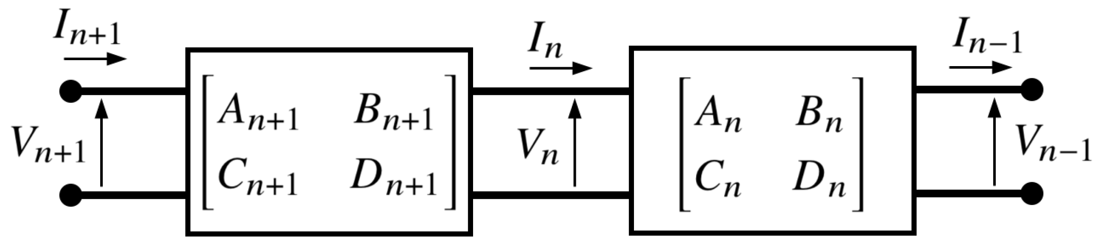
The transfer function is computed using ABCD matrices. The matrix elements corresponding to a cable are calculated from $Z_0$ and $\gamma$ as:

$$\left[\begin{array}{cc}A& B\\ C& D\end{array}\right]=\left[\begin{array}{cc}\cos \mathrm{h}(\gamma l)& Z_0\sin \mathrm{h}(\gamma l)\\ \frac{1}{Z_0}\sin \mathrm{h}(\gamma l)& \cos \mathrm{h}(\gamma l)\end{array}\right]$$

(12)

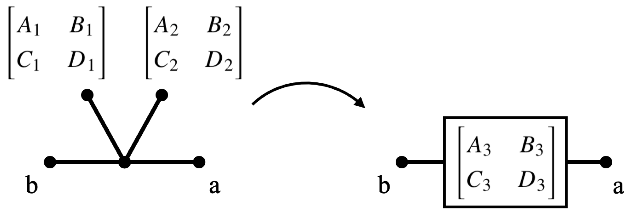
These components are computed for each cable and load, and are then combined for all the loads and wires between the transmitter and receiver. The channel transfer function (in decibels) is then calculated using (13) [16].

$$H=20lo{g}_{10}\left|\frac{R_{rec}}{A^{\prime }{R}_{rec}+B^{\prime }+R_{trans}(C^{\prime }{R}_{rec}+D^{\prime })}\right|$$

(13)

where $A^{\prime }$, $B^{\prime }$, $C^{\prime }$, $D^{\prime }$ are the matrix elements of the combined ABCD matrix, $R_{trans}$ is the transmitter impedance, and $R_{rec}$ is the receiver impedance. See the Appendix A for more details on how the transfer function is computed using two-port networks.

The network solver was written in Python and interfaced with the Bayesian inference code. The solver was verified against the code of Cañete et al. [9] for a simplified network.

3.2. Bayesian Inference

We employ a probabilistic framework to estimate model parameters based on data [21]. Specifically, we cast the inference in a Bayesian framework, which helps update our prior knowledge about the model parameters by comparing the model predictions with the available data. From the Bayes rule:

$$p(\mathit{\theta }|d)\propto p(\mathit{d}|\mathit{\theta })p(\mathit{\theta })$$

(14)

where $d\in {\mathbb{R}}^{N_d}$ is the observed data, $\mathit{\theta }$ is the set of model parameters, and $p()$ designates a probability. $p(\mathit{\theta })$ is called the prior probability and encodes any prior knowledge, including expert opinion, one might have about the model in the context of a particular application. $p(\mathit{d}|\mathit{\theta })$, called the likelihood, measures the agreement between the model and the data for select parameter values. Close agreement between the model and the data will result in higher values for the posterior $p(\mathit{\theta }|d)$.

For this work, the prior was set to a uniform distribution between the bounds set for the model parameters. We employ a Gaussian approximation for the likelihood:

$$p(\mathit{d}|\mathit{\theta })=\prod _{i=0}^{N_d}\mathcal{N}(d_i-y_i,{\sigma }^2)$$

(15)

where $y\in {\mathbb{R}}^{N_d}$ is the output of the proposed, and $\mathcal{N}(\mu ,{\sigma }^2)$ denotes a normal distribution with mean $\mu$ and variance ${\sigma }^2$. Since $\sigma$ is unknown, it is inferred as one of the parameters.

To apply Bayesian inference, parameter samples must be drawn from the prior distribution and the likelihood evaluated via (15). If the samples are drawn randomly from the prior distribution, it can take a prohibitively large number of samples to reasonably approximate the posterior, unless the number of parameters $N_{\mathit{\theta }}$ is very small. Instead, Markov chain Monte Carlo (MCMC) methods are generally used to draw samples from the distribution of $p(\mathit{d}|\mathit{\theta })$. MCMC methods take a sample and propose a modification to the sample, then estimate the likelihood at the proposed point. The proposed sample can be accepted or rejected depending on the posterior value at the new location. Therefore, samples are more likely be drawn to regions of parameter space with high posterior values. For details, see Refs. [21,36].

There are a variety of MCMC methods that could be used. Single chain methods such as the Metropolis-Hastings method [37], adaptive Metropolis (AM) [38], or delayed rejection adaptive Metropolis (DRAM) [39] update a single sample many times, making a single chain. This work uses transitional Markov chain Monte Carlo (TMCMC), which has been shown to be more robust for high dimensional parameter spaces than single chain methods [22,40,41]. TMCMC uses a series of intermediate distributions, given in (16), to  transition a set of samples from the prior to the posterior distribution:

$$\begin{array}{cc}\hfill p_j(\mathit{\theta }|d)\propto p{(d|\mathit{\theta })}^{{\beta }_j}p(\mathit{\theta }),& j=0,...,m,\hfill \\ \hfill & 0={\beta }_0<{\beta }_1<...<{\beta }_m=1\hfill \end{array}$$

(16)

${\beta }_j$ is a parameter that is increased from 0 to 1 to transition the samples gradually from the prior to the posterior. This gradual change prevents the samples from immediately clustering in locally favorable regions without exploring a larger region of parameter space.

For the PLC networks presented here, the parameters $\mathit{\theta }$ correspond to the wire length l, wire radius $r_w$, load power $P_r$, resonance frequency $f_0$, phase $\varphi$, load parameters D and T, and the standard deviation $\sigma$ for the discrepancy between the model and the data. There are additional network parameters $Q_f$, but a sensitivity analysis showed that they had marginal effects on the transfer function, so they are ignored when performing Bayesian inference to keep the parameter space lower dimensional. The load types can also be considered parameters, but they only take on discrete values and are not directly calibrated with TMCMC. Therefore, the load types are considered a separate set of discrete parameters $\Theta$ and the parameters that take on continuous values are the continuous parameters $\mathit{\theta }$. The continuous parameters have a direct dependence on the discrete parameters, so $\mathit{\theta }(\Theta )$. Furthermore, the number of continuous parameters $\mathit{\theta }$ is dependent on the discrete parameters $\Theta$ because a load will have a different number of continuous parameters depending on the load type (constant loads have one continuous parameter, frequency selective loads have two, time-varying harmonic loads have three, and time-varying commuted loads have four).

Because of the dependence of continuous parameters on discrete parameters, $\mathit{\theta }(\Theta )$, for this work we will infer $\mathit{\theta }$ for fixed $\Theta$ choices. The Bayesian inference update rule, in (14), becomes:

$$p(\mathit{\theta }|\mathit{d},\Theta )\propto p(\mathit{d}|\mathit{\theta },\Theta )p(\mathit{\theta }|\Theta )p(\Theta )$$

(17)

For simplicity, and since we are not comparing models across different sets of $\Theta$, the dependence of continuous parameters on the discrete parameters is left out of the notation in this work.

3.3. Sensitivity Analysis

We employ Global Sensitivity Analysis (GSA) to estimate how the change in network modeling output can be apportioned to changes in the continuous parameters $\mathit{\theta }$. With the focus on statistical model calibration, we employ variance-decomposition methods where the total output variance is decomposed into fractions associated with the model parameters and their interactions.

The effects of input parameters $\mathit{\theta }=\{{\mathit{\theta }}_1,\dots ,{\mathit{\theta }}_{N_{\mathit{\theta }}}\}$ and their interactions on a model output $\mathcal{M}$, are quantified through Sobol indices [42,43,44]. The first order Sobol indices are given by:

$$S_i=\frac{{\mathrm{Var}}_{{\mathit{\theta }}_i}\left[{\mathbb{E}}_{{\mathit{\theta }}_{\sim i}}(\mathcal{M}|{\mathit{\theta }}_i)\right]}{{\mathrm{Var}}_{\mathit{\theta }}\left[\mathcal{M}\right]},i=1,\cdots ,N_{\mathit{\theta }}$$

(18)

where ${\mathit{\theta }}_{\sim i}=\{{\mathit{\theta }}_1,\dots ,{\mathit{\theta }}_{i-1},{\mathit{\theta }}_{i+1},\dots ,{\mathit{\theta }}_{N_{\mathit{\theta }}}\}$, ${\mathbb{E}}_{{\mathit{\theta }}_{\sim i}}[·]$ is the expectation with respect to ${\mathit{\theta }}_{\sim i}$, and ${\mathrm{Var}}_{{\mathit{\theta }}_i}[·]$ is the variance with respect to ${\mathit{\theta }}_i$. Note that, in this context, subscript i can denote one parameter or a group of parameters. The first-order Sobol indices estimate the fractional contribution of each input parameter ${\mathit{\theta }}_i$ to the total variance of the model output.

Sobol indices are computed using UQ Toolkit [45], an open-source library for uncertainty quantification. The UQ Toolkit estimates Sobol indices using Monte Carlo (MC) algorithms proposed by Ref. [46].

3.4. Sensitivity-Informed Bayesian Inference

The network topologies in this work generally have over 50 continuous parameters $\mathit{\theta }$ that could be optimized, but a 50 parameter space is too high-dimensional to directly pursue a statistical inference study. Many of the parameters are for loads and wires far from the main path between the transmitter and receiver, and likely have an negligible effect on the transfer function. The objective of sensitivity-informed Bayesian inference is to perform Bayesian inference only on parameters that have a significant effect on the transfer function. We use Sobol indices to calculate how sensitive the frequency response is to each continuous parameter and only perform Bayesian inference on the $d_t$ most sensitive parameters. For a network with randomly generated discrete parameters $\Theta$, Sobol indices are computed for all continuous parameters $\mathit{\theta }$, then Bayesian inference is performed on a subset of $\mathit{\theta }$ designated as the trainable parameters ${\mathit{\theta }}_t\subset \mathit{\theta }$, consisting of the $d_t$ most sensitive parameters.

Sensitivity-informed Bayesian inference can only calibrate $\mathit{\theta }$ for assumed $\Theta$. Therefore, random search methods are applied to identify the discrete parameters $\Theta$ in a three-part process. First, sensitivity-informed Bayesian inference is applied to $N_{r_1}$ different realizations of the network, each with different randomly generated $\Theta$. The different realizations are independent and can be run in parallel to speed up the computational time. In the second part, further refinements are made with a random greedy search on the discrete parameters. For $N_{r_2}$ iterations, a single discrete parameter ${\Theta }_j$ is randomly regenerated, and Bayesian inference is performed only on the dependent parameters $\mathit{\theta }({\Theta }_j)$. Every third iteration, three random parameters $\mathit{\theta }$ are selected and inference is performed on them to ensure that the wires length and radius are also updated, as those parameters are not dependent on discrete parameters $\Theta$. At each stage, the new model is saved only if it is more accurate than the previous model, making it a greedy algorithm. In the third part, a single run of sensitivity-informed Bayesian inference is performed to ensure the most sensitive parameters are calibrated and to obtain an accurate sample distribution for error analysis.

To compare different calibrated models, the continuous ranked probability score (CRPS) is used [47,48,49]. CRPS provides an aggregate value expressing a prediction error for probabilistic outputs. The advantage of the CRPS over simply using the standard deviation is that it accounts for non-Gaussian distributions. See Ref. [49] for details.

The full algorithm for calibrating the network model is given in Algorithm 1.

Algorithm 1: Algorithm for calibration network model

To summarize Algorithm 1, in the initial inference step, sensitivity-informed Bayesian inference is run on a number of randomly generated network realizations. In the random search step, the most accurate model is repetitively modified, and Bayesian inference is applied only to a few parameters. In the final refinement step, sensitivity-informed Bayesian inference is applied to the most accurate model to generate parameter samples from the posterior distribution for accurate error analysis. The model calibration is all done in an offline stage, where computational resources are not a significant barrier. Model predictions of the calibrated model can then be made in an online stage very quickly.

3.5. Predictive Assessment

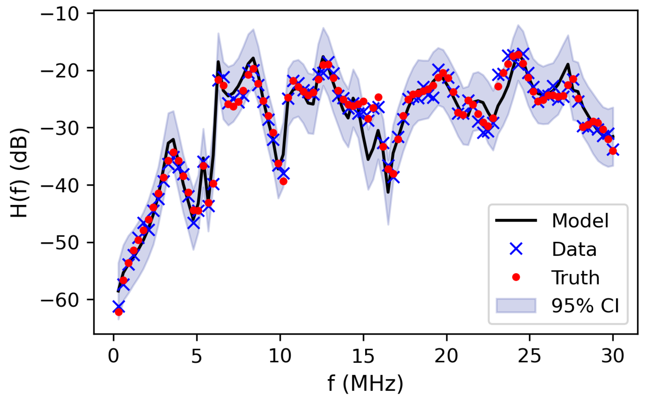
We will employ both pushed-forward distributions and Bayesian posterior-predictive distributions [50] to assess the predictive skill of the transfer function. The pushed-forward distribution is the model distribution computed directly from the samples, and the Bayesian posterior-predictive distribution is the model distribution inclusive of the statistical discrepancy between the model and the data (and therefore accounts for model form and/or measurements errors). The process used to generate push-forward posterior estimates is formalized as:

$$\begin{array}{c}\hfill p(\mathit{\theta }|\mathit{d})\to \{\underset{\mathrm{Posterior Samples}}{\underbrace{{\mathit{\theta }}^{(1)},\dots ,{\mathit{\theta }}^{(m)}}}\}\stackrel{H(\mathit{\theta })}{\to }\{{\mathit{d}}^{(\mathrm{pf},1)},\dots ,{\mathit{d}}^{(\mathrm{pf},m)}\}\to p_{\mathrm{pf}}({\mathit{d}}^{(\mathrm{pf})}|\mathit{d}).\end{array}$$

(19)

Here, ${\mathit{d}}^{(\mathrm{pf})}$ denotes hypothetical data and $p_{\mathrm{pf}}({\mathit{d}}^{(\mathrm{pf})}|\mathit{d})$ denotes the push-forward probability density of the hypothetical data ${\mathit{d}}^{(\mathrm{pf})}$ conditioned on the observed data $\mathit{d}$. We start with samples from the posterior distribution $p(\mathit{\theta }|\mathit{d})$. These samples are readily available from the TMCMC exploration of the parameter space. Using these samples, we evaluate the transfer function H and collect the resulting ${\mathit{d}}^{(\mathrm{pf})}=H(\mathit{\theta })$ samples that correspond to the push-forward posterior distribution $p_{\mathrm{pf}}({\mathit{d}}^{(\mathrm{pf})}|\mathit{d})$.

The pushed-forward posterior does not account for the discrepancy between the data $\mathit{d}$ and the model predictions, subsumed into the definition of the likelihood function in (15). The Bayesian posterior-predictive distribution, defined in (20), is computed by marginalization of the likelihood over the posterior distribution of model parameters $\mathit{\theta }$:

$$p_{\mathrm{pp}}\left({\mathit{y}}^{(\mathrm{pp})}|\mathit{d}\right)={\int }_{\mathit{\theta }}p({\mathit{y}}^{(\mathrm{pp})}|\mathit{\theta })p(\mathit{\theta }|\mathit{d})d\mathit{\theta }.$$

(20)

In practice, we estimate $p_{\mathrm{pp}}\left({\mathit{y}}^{(\mathrm{pp})}|\mathit{d}\right)$ through sampling. The sampling workflow is similar to the one shown in (19). After the model evaluations $\mathit{d}=H(\theta )$ are completed, we add random noise consistent with the likelihood model settings presented in (15). The resulting samples are used to compute summary statistics of $p_{\mathrm{pp}}\left({\mathit{d}}^{(\mathrm{pp})}|\mathit{d}\right)$. For example, the modeled transfer function is the mean of $p_{\mathrm{pp}}\left({\mathit{d}}^{(\mathrm{pp})}|\mathit{d}\right)$.

4. Results

All results shown here are for the network topology shown in Figure 2. Bayesian inference is done using the network frequency response for four combinations of the transmitter and receiver resistances at 20 $\Omega$ and 100 $\Omega$. The frequency response computed at the different resistances and different times is concatenated to form the model output. To test the inference methodology, it is more appropriate to use simulation data rather than actual measurements in order that the parameters of the model are known exactly. Therefore, the “true” network transfer function is calculated with a set of randomly generated $\Theta$ and $\mathit{\theta }$. Noise is added to the “true” transfer function to simulate experimental measurement noise. The noise is zero mean Gaussian noise with a standard deviation on $0.1$ dB. The resulting data $\mathit{d}$ is then used to calibrate the network model.

There are several algorithm parameters that must be determined, namely $N_{s_1}$, $N_{s_2}$, $N_{r_1}$, $N_{r_2}$, and $d_t$. A convergence study was done to ensure that a sufficient number of samples is used in TMCMC and that a sufficient number of parameters are optimized during the Bayesian inference. The convergence study found that using $N_{s_1}=30,000$, $N_{s_2}=300$ and optimizing the $d_t=20$ most sensitive parameters resulted in accurate inferences. The number of realizations were set at $N_{r_1}=10$ and $N_{r_2}=200$. A larger number of realizations did not improve the model. For computing Sobol indices, 3000 samples were drawn for each dimension of parameter space. For brevity the convergence study is not shown here. All results shown are from the final refinement step of Algorithm 1.

This section is organized as follows: Section 4.1 examines Sobol indices of parameters from a baseline case, and Section 4.2 examines marginal distributions in the parameter space. Section 4.3 shows results on the baseline case and Section 4.4 shows results in an extrapolative scenario. Section 4.5 shows results from 30 different realizations to show how reliably network parameters are inferred.

4.1. Sensitivity Analysis

The Sobol indices are computed in the final refinement step of Algorithm 1 to identify the most sensitive parameters.

Table 2. Parameters in Figure 3. The node names are from Figure 2.

Parameter	Parameter Type	Connecting Nodes	Sobol Index
${\theta }_1$	Load $P_r$	L4-3	0.627
${\theta }_2$	Load $f_0$	L4-3	0.199
${\theta }_3$	Wire l	JB4–L4-1	0.021
${\theta }_4$	Wire l	SP–JB2	0.016
${\theta }_5$	Wire l	SP–JB3	0.013
${\theta }_6$	Wire l	SP–JB4	0.012
${\theta }_7$	Load $P_r$	L1-3	0.011
${\theta }_8$	Wire l	SP–JB1	0.011
${\theta }_9$	Load D	L4-3	0.010
${\theta }_{10}$	Load $P_r$	L4-1	0.010
${\theta }_{11}$	Wire l	JB4–L4-3	0.010
${\theta }_{12}$	Load $f_0$	L4-1	0.009
${\theta }_{13}$	Wire l	L4-3–Receiver	0.009
${\theta }_{14}$	Wire l	JB2–L2-1	0.009
${\theta }_{15}$	Wire l	JB2–L2-3	0.008
${\theta }_{16}$	Wire l	L4-1–L4-2	0.006
${\theta }_{17}$	Wire l	JB1–L1-3	0.006
${\theta }_{18}$	Load $P_r$	L2-1	0.006
${\theta }_{19}$	Load T	L4-3	0.006
${\theta }_{20}$	Wire l	JB1–Transmitter	0.005

shows the 20 most sensitive parameters for the calibrated model of a single network realization along with the corresponding Sobol indices. The two most sensitive parameters are the load power and resonance frequency of load L4-3, which is the only load directly adjacent to the main path between transmitter and receiver. All other parameters have Sobol indices below 0.021, but the 20 most sensitive parameters have Sobol indices about 0.005. Note that parameters with a low Sobol index can still be important to the model. Sobol indices measure the importance of each parameter to the overall output variance, and the L4-3 load power is most important in determining the magnitude of the transfer function, i.e., changing load power will change the magnitude, but not significantly affect the shape of the transfer function. However, the other parameters need to be calibrated to accurately model the frequency dependence of the transfer function.

4.2. Marginal Parameter Distributions

The Bayesian methods used to calibrate the PLC model are equipped to deal with heterogeneous sources of uncertainty, in this case from our modeling assumptions, i.e., model and parametric uncertainties, as well as experimental errors. The samples drawn from the posterior can be used to examine the correlations between model parameters and the impact of modeling assumptions on the predictive capabilities of the model. Here, the samples are used to compute marginal density functions using kernel density estimation [51,52] with a Gaussian kernel.

The 1D and 2D marginal density functions are shown in Figure 3 for the 20 most sensitive parameters listed in Table 2. The logarithm of $\sigma$ is included as the final parameter. The plots on the diagonal of Figure 3 show the 1D density functions normalized such that the values are between 0 and 1. The off-diagonal plots show the 2D joint marginals for pairs of parameters. Some of the off-diagonal plots exhibit a skewed marginal density, suggesting some level of correlation for the corresponding pair of parameters. For example, parameters 4 and 15 (fifteenth row, fourth column) show a negative correlation. These parameters are wire lengths of adjacent wires, so it is not surprising that they are correlated. There are also correlations between the load power and frequency of load L4-3 (second row, first column), as well as several wires connected to the service panel (${\theta }_6$, ${\theta }_8$). Uncertainty quantification methods often assume uncorrelated parameter distributions, which sometimes leads to summary statistics that are wider than expected. Accounting for correlations or dependencies between model parameters in a Bayesian framework will lead to more accurate error bounds.

4.3. Network Inference

Figure 4 shows the modeled transfer function computed from the calibrated model at $R_{rec}=R_{trans}=100\Omega$. The error bounds shown are the 95% confidence intervals computed from the standard deviation of $p_{\mathrm{pp}}\left({\mathit{y}}^{(\mathrm{pp})}|\mathit{d}\right)$. The calibrated model reproduces the true data reasonably well despite being trained on the noisy data. Slight discrepancies are observed at approximately 15 MHz, but the modeled transfer function generally captures the peak frequencies accurately.

Figure 5 shows the model transfer function at each of the four transmitter/receiver resistance combinations along with the true data. The model replicates the true transfer function accurately for each different set of resistances.

It is of interest to know how accurate the calibrated model is at identifying load and wire parameters.

Table 3. Load types, load power, and resonance frequency for the true model and calibrated model. The node names are from Figure 2.

Load	Load Type		Load Power (W)		Resonance Freq (MHz)
	True	Model	True	Model	True	Model
L1-1	Constant	Time-varying harmonic	13.2	22.7	-	7.5
L1-2	Constant	Time-varying harmonic	38.1	65.1	-	23.6
L1-3	Time-varying harmonic	Constant	69.0	414.1	11.1	-
L2-1	Frequency selective	Time-varying commuted	54.2	243.3	28.9	18.2
L2-2	Time-varying commuted	Frequency selective	37.7	5.2	24.0	19.0
L2-3	Constant	Frequency selective	9.4	27.6	-	18.8
L2-4	Frequency selective	Frequency selective	51.5	282.5	21.4	15.5
L3-1	Time-varying harmonic	Time-varying commuted	51.0	37.7	23.9	20.5
L3-2	Frequency selective	Time-varying commuted	96.6	245.5	19.0	3.5
L3-3	Time-varying harmonic	Time-varying harmonic	18.0	132.4	19.9	16.9
L3-4	Time-varying commuted	Constant	471.7	73.0	6.6	-
L4-1	Time-varying commuted	Frequency selective	76.0	173.6	18.7	12.9
L4-2	Time-varying harmonic	Time-varying commuted	90.4	66.1	6.5	16.2
L4-3	Time-varying commuted	Time-varying commuted	14.6	9.4	16.5	17.7

shows the load types and several load parameters (load power and resonance frequency) for the true network and calibrated model. The model correctly inferred the load type of L4-3 and accurately identified the load power and resonance frequency for that load. However, the load types are less accurately identified for most other loads. Note that load L4-3 is the only load directly adjacent to the main path between the transmitter and receiver. Overall, eight of the fourteen (57%) loads types are modeled correctly, but if the model randomly chose load types, only 25% of them would be correct. The load parameters of most loads are highly inaccurate as a result of the load types being inaccurate.

A similar comparison of wire radii and wire lengths is shown in

Table 4. Wire radius and length for the true model and calibrated model. The node names are from Figure 2.

Connecting Nodes	Wire Radius (mm)			Wire Length (m)
	True	Model	%Errorr	True	Model	%Errorr
SP–JB1	1.47	1.85	18.1%	5.39	5.67	1.8%
SP–JB2	1.46	1.04	20.0%	9.96	10.59	4.2%
SP–JB3	1.24	1.88	31.2%	14.29	14.38	0.6%
SP–JB4	1.33	1.42	4.35%	9.00	9.36	2.4%
JB1–Transmitter	1.07	1.14	13.1%	3.31	3.46	5.1%
JB1–L1-1	1.01	1.17	33.8%	2.53	2.13	13.3%
JB1–L1-2	0.86	1.16	62.1%	2.66	4.47	60.4%
JB1–L1-3	1.29	1.22	14.4%	2.36	2.52	5.4%
JB2–L2-1	1.02	1.05	7.3%	4.33	4.34	0.4%
L2-1– L2-2	1.17	1.03	28.9%	3.29	3.94	21.6%
JB2–L2-3	1.06	1.06	0.2%	3.07	3.93	28.6%
L2-3– L2-4	1.25	1.05	41.8%	2.02	2.56	18.0%
JB3–L3-1	1.05	1.00	10.6%	3.24	3.89	21.6%
JB3–L3-2	1.20	0.99	43.6%	2.69	2.23	15.1%
JB3–L3-3	1.17	1.11	12.7%	4.40	4.25	4.9%
JB3–L3-4	1.28	1.04	50.3%	4.75	3.98	25.7%
JB4–L4-1	0.93	1.15	45.6%	2.56	4.99	81.0%
L4-1– L4-2	1.19	0.90	59.6%	3.59	5.00	46.9%
JB4–L4-3	0.89	1.19	62.5%	4.61	2.01	86.9%
L4-3– Receiver	0.94	0.89	5.5%	4.23	4.18	1.41%

. The error shown is normalized by the total range, shown in Equation (21). This is done because the wires can have different lengths depending on the position in the network, as explained in Section 2.3.

$$\%Erro{r}_r=100\%·\frac{|True-Model|}{Max-Min}$$

(21)

It should be noted that the $\%Erro{r}_r$ can vary between 0% and 100%, and has a mean of 33.3% if both the true and model values are chosen randomly. The error normalized by the range therefore gives more information on whether parameters are actually inferred than error normalized by the true value. Table 4 shows that for most wires, the model is poor at identifying both radius and length. However, the model identifies the wire length with reasonable accuracy for four wires connected to the service panel. This is a high dimensional system and with noisy training data, so it is unsurprising that the model incorrectly identifies many of the parameters.

4.4. Model Predictions at Other Resistances

A more rigorous test of the calibrated model is determining its accuracy when extrapolating. The calibrated network model is physics-based, meaning the model uses equations based on the underlying physics of the network topology and TL theory. Physics-based models have been found to perform better than basic data-fitting methods in many physical science applications [53]. One benefit of physics-based models is that they generally perform better when the inputs are outside the range of the training data, whereas non-physics-based data fitting methods such as machine learning generally give highly inaccurate predictions under extrapolative scenarios.

In this section, the calibrated model is tested with different transmitter and receiver resistances in extrapolative scenarios. In Figure 6, the transfer function of the inferred model is calculated with four transmitter and receiver resistance combinations at resistances of $10\Omega$ and $400\Omega$. Despite being trained on transmitter/receiver resistances at $20\Omega$ and $100\Omega$, the model is very accurate at the other resistances. Slight inaccuracies are observed in the 15–20 MHz range, particularly for the $R_{trans}=400\Omega$, $R_{rec}=10\Omega$ case. However, the model generally gives very accurate predictions within the model error bounds.

For comparison, the transfer functions for four cases when the transmitter and receiver resistances are equal are plotted together in Figure 7. A non-physics-based model would have to predict the transfer function at $R_{trans}=R_{rec}=10$ and $R_{trans}=R_{rec}=400$ based on the other two transfer functions, whereas the model presented here can use data when the transmitter and receiver resistances are not equal to improve the model. Note that there are many frequencies when trends between different resistances are difficult or impossible to predict just based on the $20\Omega$ and $100\Omega$ cases; for example at 3 MHz, the transfer function at $R_{trans}=R_{rec}=100\Omega$ and $20\Omega$ are almost equal, but is lower at $400\Omega$ and $10\Omega$. This trend would be impossible to predict using non-physics-based models with data only at $20\Omega$ and $100\Omega$, but is accurately predicted using the calibrated model.

4.5. Statistical Analysis of Multiple Network Realizations

The results shown previously all use a single realization of the network to analyze how accurately the model parameters are inferred. Here calibrations are done for 30 different realizations of the network to analyze statistically how accurately the calibration infers network parameters.

Figure 8 shows the true and modeled transfer function at $R_{trans}=R_{rec}=100\Omega$ for the first ten realizations. In each realization, the modeled transfer function accurately reproduces the true transfer function, showing that the calibration method is robust. From the earlier analysis of a single realization, the only load that was accurately inferred was load L4-3, so it is of particular interest to know how well the network infers that load.

Table 5. Load types, load power, and resonance frequency for load L4-3 of the true and calibrated model for 15 realizations.

Model #	Load Type		Load Power (W)		Resonance Freq (MHz)
	True	Model	True	Model	True	Model
1	Time-varying commuted	Time-varying commuted	14.6	9.35	16.5	17.7
2	Time-varying harmonic	Frequency selective	322.5	32.0	7.06	4.01
3	Constant	Constant	18.0	35.4	-	-
4	Time-varying harmonic	Time-varying harmonic	11.1	33.3	21.9	21.0
5	Frequency selective	Constant	17.2	92.7	7.3	-
6	Constant	Constant	293.4	279.2	-	-
7	Frequency selective	Frequency selective	319.9	930.7	21.6	21.0
8	Constant	Constant	63.5	33.4	-	-
9	Constant	Constant	44.2	67.5	-	-
10	Time-varying commuted	Time-varying commuted	3078.6	3760.7	27.8	28.1
11	Frequency selective	Frequency selective	3179.7	4770.6	9.5	9.3
12	Constant	Frequency selective	19.5	6.0	-	3.0
13	Time-varying harmonic	Time-varying harmonic	128.4	42.2	21.3	18.4
14	Time-varying commuted	Time-varying commuted	271.4	267.5	14.3	14.7
15	Time-varying harmonic	Time-varying harmonic	29.2	231.6	11.4	10.4

shows the load type, power, and resonance frequency of load L4-3 for the first 15 realizations (for brevity only 15 are shown). Most load type and resonance frequencies are estimated well by the model. The modeled load power is less accurately inferred, but is always within a factor of $8\times$. For reference, the load power can vary by a factor of $1000\times$, so load power is reasonably well inferred. Out of the 30 realizations, the load type was correctly inferred in 23 of them (77%).

Table 6. Average errors (in %) for wire length and radius from the 30 realizations. The node names are from Figure 2.

Connecting Nodes	Wire Radius	Wire Length
	Mean %Errorr	Mean %Errorr
SP–JB1	19%	26%
SP–JB2	16%	26%
SP–JB3	17%	27%
SP–JB4	15%	24%
JB1–Transmitter	30%	7%
JB1–L1-1	32%	28%
JB1–L1-2	36%	34%
JB1–L1-3	35%	22%
JB2–L2-1	24%	42%
L2-1– L2-2	37%	22%
JB2–L2-3	32%	26%
L2-3– L2-4	35%	26%
JB3–L3-1	30%	30%
JB3–L3-2	36%	31%
JB3–L3-3	31%	36%
JB3–L3-4	37%	22%
JB4–L4-1	30%	21%
L4-1– L4-2	31%	29%
JB4–L4-3	29%	32%
L4-3–Receiver	40%	12%

shows the $\%Erro{r}_r$ for wire radius and wire length averaged over the 30 realizations. The 95% confidence intervals of $\%Erro{r}_r$ are $\pm 8\%$ for both wire radius and wire length, calculated from the standard deviation of $\%Erro{r}_r$ and averaging the confidence intervals over every wire. Table 6 indicates that the calibration is able to infer information about wire radius only for wires connected to the service panel. However, information on wire length is inferred for wires connected to the service panel, transmitter, and receiver. The average $\%Erro{r}_r$ for all wires except those connected to the service panel, transmitter, and receiver is 32.3% for wire radius and 28.6% for wire length. Since $\%Erro{r}_r$ is 33.3% for random guessing, this indicates that the method presented here is unable to infer wire radius for any of the wires not connected to the service panel, transmitter, and receiver, and is not consistently inferring wire length data for those wires.

Though the calibration is able to infer wire parameters of the wires connected to the service panel, transmitter, and receiver, they are less accurate than parameters of load L4-3. This is likely because there are unobserved latent variables in the network that have more control over the transfer function. The wires are likely closely coupled throughout the network in such a way that the network transfer function is accurate even though individual wires may not be inferred accurately. For example, the wires connecting the service panel to nodes JB1 and JB4 are both on the main path between transmitter and receiver, so it is possible that for certain realizations, the combined length of those two wires is more important than the individual lengths. The average absolute error $|True-Model|$ for the length of wire SP–JB1 is 3.9 m and the average error for wire SP–JB4 is 3.6 m. However, the average error when the wire lengths are added is 3.7 m, even though the combined wire length has a larger range of 10–40 m instead of 5–20 m for the single wires, and therefore the error on the sum of the wire lengths would be larger if the wire lengths are independent.

This analysis has shown that the calibrated model can infer some network parameters, mainly those on the main path between transmitter and receiver. Despite inaccuracies in the inferred parameters, the calibrated model accurately computes the transfer function for the network even under extrapolative scenarios.

5. Conclusions

Bayesian inference is used to calibrate a home network PLC model when the loads and wires are unknown. The model uses TL theory to calculate the network transfer function, resulting in a physics-based model similar to bottom-up models, but that can be calibrated to specific networks. The calibration uses Sobol indices to select the most sensitive parameters and then applies Bayesian inference on the selected parameters. Further refinements to calibrate the load and wire types are done through a greedy random search that regenerates individual load types and applies Bayesian inference on the dependent continuous parameters.

The resulting model can accurately reproduce the true transfer function despite being trained on noisy data. The model is also shown to be accurate in extrapolative scenarios. The calibrated model is most accurate at inferring the load closest to the main path between transmitter and receiver, and it can also infer some knowledge of wire parameters also on the main path. However, many of the other model parameters are inaccurate due to several reasons. The model is high dimensional, containing 15 loads and 20 wires, each of which contain one to five parameters. The training data is a vector of dimension 4000, but most of the points are highly correlated, so the training data can be considered fairly low dimensional. As a result, there are likely many model parameter combinations that satisfy or nearly satisfy the training data. In addition, the training data has noise, so even the correct parameters from the true model may not be optimal for the training data. Finally, the sensitivity-informed Bayesian inference method presented here can only identify continuous parameters accurately, but the load types (discrete parameters) are identified through random searches which are unlikely to find the true load and wire types.

There are a number of possible directions for future works to take. Future works could target improving the calibration process, as the method presented here has shortcomings; in particular, the method of identifying load types could use improvement. Future works could also use more realistic network topology models as well as more complex loads. The wire model used here is very simple, so more complex wire models with discrete valued parameters could be used. More complex PLC models could be used that incorporate noise and signal filtering. In addition, models could incorporate signal couplers between low voltage and medium voltage networks. Future studies could use the calibrated model to examine the effects of disturbances in the power grid such as voltage dips and brief power outages. Future works could also target gaining more information from the network to improve the model, and developing models when the network topology is only partially known. Future work is planned to take measurements and use the method presented here to develop a model.

References

1. Galli, S.; Scaglione, A.; Wang, Z. For the grid and through the grid: The role of power line communications in the smart grid. Proc. IEEE 2011, 99, 998–1027. [Google Scholar] [CrossRef] [Green Version]
2. Nassar, M.; Lin, J.; Mortazavi, Y.; Dabak, A.; Kim, I.H.; Evans, B.L. Local utility power line communications in the 3–500 kHz band: Channel impairments, noise, and standards. IEEE Signal Process. Mag. 2012, 29, 116–127. [Google Scholar] [CrossRef]
3. Sonmez, M.A.; Zehir, M.A.; Bagriyanik, M.; Nak, O. Impulsive noise survey on power line communication networks up to 125 kHz for smart metering infrastructure in systems with solar inverters in Turkey. In Proceedings of the 2013 International Conference on Renewable Energy Research and Applications (ICRERA), Madrid, Spain, 20–23 October 2013; pp. 705–710. [Google Scholar]
4. Coelho, P.; Gomes, M.; Moreira, C. Smart metering technology. In Microgrids Design and Implementation; Springer: Berlin/Heidelberg, Germany, 2019; pp. 97–137. [Google Scholar]
5. Van de Kaa, G.; Fens, T.; Rezaei, J.; Kaynak, D.; Hatun, Z.; Tsilimeni-Archangelidi, A. Realizing smart meter connectivity: Analyzing the competing technologies power line communication, mobile telephony, and radio frequency using the best worst method. Renew. Sustain. Energy Rev. 2019, 103, 320–327. [Google Scholar] [CrossRef]
6. Mlỳnek, P.; Rusz, M.; Benešl, L.; Sláčik, J.; Musil, P. Possibilities of broadband power line communications for smart home and smart building applications. Sensors 2021, 21, 240. [Google Scholar] [CrossRef] [PubMed]
7. Masood, B.; Khan, M.A.; Baig, S.; Song, G.; Rehman, A.U.; Rehman, S.U.; Asif, R.M.; Rasheed, M.B. Investigation of deterministic, statistical and parametric NB-PLC channel modeling techniques for advanced metering infrastructure. Energies 2020, 13, 3098. [Google Scholar] [CrossRef]
8. Lopez, G.; Matanza, J.; De La Vega, D.; Castro, M.; Arrinda, A.; Moreno, J.I.; Sendin, A. The role of power line communications in the smart grid revisited: Applications, challenges, and research initiatives. IEEE Access 2019, 7, 117346–117368. [Google Scholar] [CrossRef]
9. Canete, F.J.; Cortes, J.A.; Diez, L.; Entrambasaguas, J.T. A channel model proposal for indoor power line communications. IEEE Commun. Mag. 2011, 49, 166–174. [Google Scholar] [CrossRef]
10. Tonello, A.M.; Versolatto, F. Bottom-up statistical PLC channel modeling—Part I: Random topology model and efficient transfer function computation. IEEE Trans. Power Deliv. 2011, 26, 891–898. [Google Scholar] [CrossRef]
11. Tonello, A.M.; Versolatto, F.; Béjar, B.; Zazo, S. A fitting algorithm for random modeling the PLC channel. IEEE Trans. Power Deliv. 2012, 27, 1477–1484. [Google Scholar] [CrossRef] [Green Version]
12. Phillipps, H. Modelling of powerline communication channels. In Proceedings of the 3rd International Symposium on Power-Line Communications and its Applications (ISPLC’99), Lancaster, UK, 30 March–1 April 1999; pp. 14–21. [Google Scholar]
13. Zimmermann, M.; Dostert, K. A multipath model for the powerline channel. IEEE Trans. Commun. 2002, 50, 553–559. [Google Scholar] [CrossRef] [Green Version]
14. Zhu, W.; Zhu, X.; Lim, E.; Huang, Y. State-of-art power line communications channel modelling. Procedia Comput. Sci. 2013, 17, 563–570. [Google Scholar] [CrossRef] [Green Version]
15. Frickey, D.A. Conversions between S, Z, Y, H, ABCD, and T parameters which are valid for complex source and load impedances. IEEE Trans. Microw. Theory Tech. 1994, 42, 205–211. [Google Scholar] [CrossRef]
16. Marrocco, G.; Statovci, D.; Trautmann, S. A PLC broadband channel simulator for indoor communications. In Proceedings of the 2013 IEEE 17th International Symposium on Power Line Communications and Its Applications, Johannesburg, South Africa, 24–27 March 2013; pp. 321–326. [Google Scholar]
17. Fang, X.; Wang, N.; Gulliver, T.A. A PLC channel model for home area networks. Energies 2018, 11, 3344. [Google Scholar] [CrossRef] [Green Version]
18. Aalamifar, F.; Schlögl, A.; Harris, D.; Lampe, L. Modelling power line communication using network simulator-3. In Proceedings of the 2013 IEEE Global Communications Conference (GLOBECOM), Atlanta, GA, USA, 9–13 December 2013; pp. 2969–2974. [Google Scholar]
19. Passerini, F.; Righini, D.; Tonello, A.M. A bottom-up PLC channel model that includes radiation effects. In Proceedings of the 2018 IEEE International Symposium on Power Line Communications and its Applications (ISPLC), Manchester, UK, 8–11 April 2018; pp. 1–6. [Google Scholar]
20. Masood, B.; Haider, A.; Baig, S. Modeling and characterization of low voltage access network for narrowband powerline communications. J. Electr. Eng. Technol. 2017, 12, 443–450. [Google Scholar] [CrossRef] [Green Version]
21. Gilks, W.R.; Richardson, S.; Spiegelhalter, D.J. Markov Chain Monte Carlo in Practice; Chapman and Hall: London, UK, 1996. [Google Scholar]
22. Ching, J.; Chen, Y.C. Transitional Markov chain Monte Carlo method for Bayesian model updating, model class selection, and model averaging. J. Eng. Mech. 2007, 133, 816–832. [Google Scholar] [CrossRef]
23. Huang, Y.X.; Zhang, X.D.; Yu, F.; Wei, Y.Q.; Zhang, H.L. Networking of smart meters based on time-varying feature of low-voltage power line channel in microgrid. Complexity 2021, 2021. [Google Scholar] [CrossRef]
24. Ferreira, H.C.; Lampe, L.; Newbury, J.; Swart, T.G. Power Line Communications: Theory and Applications for Narrowband and Broadband Communications Over Power Lines; John Wiley & Sons: Hoboken, NJ, USA, 2010. [Google Scholar]
25. Paul, C.R. Analysis of Multiconductor Transmission Lines; John Wiley & Sons: Hoboken, NJ, USA, 2007. [Google Scholar]
26. Panduit. Electrical Wire Sizes Selection Guide. 2011. Available online: http://www.panduit.com/heiler/SelectionGuides/WW-WASG03%20Electrical%20Wire%20Sizes-WEB%207-7-11.pdf (accessed on 20 April 2021).
27. Gruber, F.; Lampe, L. On PLC channel emulation via transmission line theory. In Proceedings of the 2015 IEEE International Symposium on Power Line Communications and Its Applications (ISPLC), Austin, TX, USA, 29 March–1 April 2015; pp. 178–183. [Google Scholar]
28. Cortés, J.A.; Canete, F.J.; Diez, L.; Torres, L.M.; Hispania, S.M. On PLC channel models: An OFDM-based comparison. In Proceedings of the 2013 IEEE 17th International Symposium on Power Line Communications and Its Applications, Johannesburg, South Africa, 24–27 March 2013; pp. 333–338. [Google Scholar]
29. Grenander, U.; Miller, M.I. Representations of knowledge in complex systems. J. R. Stat. Soc. Ser. B 1994, 56, 549–581. [Google Scholar] [CrossRef]
30. Green, P.J. Reversible jump Markov chain Monte Carlo computation and Bayesian model determination. Biometrika 1995, 82, 711–732. [Google Scholar] [CrossRef]
31. Corchado, J.A.; Cortés, J.A.; Canete, F.J.; Díez, L. An MTL-based channel model for indoor broadband MIMO power line communications. IEEE J. Sel. Areas Commun. 2016, 34, 2045–2055. [Google Scholar] [CrossRef]
32. U.S. Department of Energy. Estimating Appliance and Home Electronic Energy Use. 2020. Available online: https://www.energy.gov/energysaver/save-electricity-and-fuel/appliances-and-electronics/estimating-appliance-and-home (accessed on 20 April 2021).
33. Wholesale Solar. How Much Power Do Your Appliances Use? 2020. Available online: https://www.wholesalesolar.com/solar-information/power-table (accessed on 20 April 2021).
34. Matanuska Electric Association. Common Household Appliance Energy Use. 2014. Available online: http://www.mea.coop/wp-content/uploads/2014/06/High-Bill-Packet.pdf (accessed on 20 April 2021).
35. Golden, P.; Dedieu, H.; Jacobsen, K.S. Fundamentals of DSL Technology; CRC Press: Boca Raton, FL, USA, 2005. [Google Scholar]
36. Geyer, C.J. Practical Markov chain Monte Carlo. Stat. Sci. 1992, 7, 473–483. [Google Scholar] [CrossRef]
37. Chib, S.; Greenberg, E. Understanding the Metropolis-Hastings algorithm. Am. Stat. 1995, 49, 327–335. [Google Scholar]
38. Haario, H.; Saksman, E.; Tamminen, J. An adaptive Metropolis algorithm. Bernoulli 2001, 7, 223–242. [Google Scholar] [CrossRef] [Green Version]
39. Haario, H.; Laine, M.; Mira, A.; Saksman, E. DRAM: Efficient adaptive MCMC. Stat. Comput. 2006, 16, 339–354. [Google Scholar] [CrossRef]
40. Betz, W.; Papaioannou, I.; Straub, D. Transitional Markov chain Monte Carlo: Observations and improvements. J. Eng. Mech. 2016, 142, 04016016. [Google Scholar] [CrossRef] [Green Version]
41. Ching, J.; Wang, J.S. Application of the transitional Markov chain Monte Carlo algorithm to probabilistic site characterization. Eng. Geol. 2016, 203, 151–167. [Google Scholar] [CrossRef]
42. Sobol, I.M. On sensitivity estimation for nonlinear mathematical models. Mat. Model. 1990, 2, 112–118. [Google Scholar]
43. Saltelli, A.; Tarantola, S.; Campolongo, F. Sensitivity analysis as an ingredient of modeling. Stat. Sci. 2000, 15, 377–395. [Google Scholar]
44. Sobol, I.M. Global sensitivity indices for nonlinear mathematical models and their Monte Carlo estimates. Math. Comput. Simul. 2001, 55, 271–280. [Google Scholar] [CrossRef]
45. Sargsyan, K.; Safta, C.; Chowdhary, K.S.; Castorena, S.; De Bord, S.; Debusschere, B. UQTk Version 3.0 User Manual; Technical Report; Sandia National Lab.: Livermore, CA, USA, 2016.
46. Saltelli, A. Making best use of model evaluations to compute sensitivity indices. Comput. Phys. Commun. 2002, 145, 280–297. [Google Scholar] [CrossRef]
47. Brown, T.A. Admissible Scoring Systems for Continuous Distributions; The Rand Corporation: Santa Monica, CA, USA, 1974. [Google Scholar]
48. Matheson, J.E.; Winkler, R.L. Scoring rules for continuous probability distributions. Manag. Sci. 1976, 22, 1087–1096. [Google Scholar] [CrossRef]
49. Hersbach, H. Decomposition of the continuous ranked probability score for ensemble prediction systems. Weather. Forecast. 2000, 15, 559–570. [Google Scholar] [CrossRef]
50. Lynch, S.M.; Western, B. Bayesian posterior predictive checks for complex models. Sociol. Methods Res. 2004, 32, 301–335. [Google Scholar] [CrossRef] [Green Version]
51. Rosenblatt, M. Remarks on some nonparametric estimates of a density function. Ann. Math. Stat. 1956, 27, 832–837. [Google Scholar] [CrossRef]
52. Parzen, E. On estimation of a probability density function and mode. Ann. Math. Stat. 1962, 33, 1065–1076. [Google Scholar] [CrossRef]
53. Carleo, G.; Cirac, I.; Cranmer, K.; Daudet, L.; Schuld, M.; Tishby, N.; Vogt-Maranto, L.; Zdeborová, L. Machine learning and the physical sciences. Rev. Mod. Phys. 2019, 91, 045002. [Google Scholar] [CrossRef] [Green Version]
Figure 1. Schematic of room wiring connection types.
Energies 14 02402 g001
Figure 2. Schematic of network topology. Junction boxes are designated as JBx and loads are designated Lx-y, where x is the room number and y is the load number in the room.
Energies 14 02402 g002
Figure 3. Marginal distributions of 20 parameters from last TMCMC calibration.
Energies 14 02402 g003
Figure 4. Calibrated model transfer function at R r e c = R t r a n s = 100 Ω . The results shown are at the first discrete time t = 0 . The blue symbols are the true transfer function and the red symbols are the transfer function with added noise.
Energies 14 02402 g004
Figure 5. Calibrated model transfer function (lines) and true transfer function (symbols) at various resistances.
Energies 14 02402 g005
Figure 6. Inferred model transfer function (lines) and true transfer function (symbols) at various transmitter and receiver resistances.
Energies 14 02402 g006
Figure 7. True transfer function for various resistances.
Energies 14 02402 g007
Figure 8. Calibrated model transfer function (lines) and true transfer function (symbols) at R t r a n s = R r e c = 100 Ω for 10 different realizations.
Energies 14 02402 g008