Abstract
Solar irradiance forecasting is an inevitable and most significant process in grid-connected photovoltaic systems. Solar power is highly non-linear, and thus to manage the grid operation efficiently, with irradiance forecasting for various timescales, such as an hour ahead, a day ahead, and a week ahead, strategies are developed and analysed in this article. However, the single time scale model can perform better for that specific time scale but cannot be employed for other time scale forecasting. Moreover, the data consideration for single time scale forecasting is limited. In this work, a multi-time scale model for solar irradiance forecasting is proposed based on the multi-task learning algorithm. An effective resource sharing scheme between each task is presented. The proposed multi-task learning algorithm is implemented with a long short-term memory (LSTM) neural network model and the performance is investigated for various time scale forecasting. The hyperparameter estimation of the proposed LSTM model is made by a hybrid chicken swarm optimizer based on combining the best features of both the chicken swarm optimization algorithm (CSO) and grey wolf optimization (GWO) algorithm. The proposed model is validated, comparing existing methodologies for single timescale forecasting, and the proposed strategy demonstrated highly consistent performance for all time scale forecasting with improved metric results.
1. Introduction
Renewable energy resources have gained significance in the context of power sector applications to balance energy demand and generation [1]. The energy crisis is a serious problem encountered by all countries in the world. The growth and development of renewable energy sources are major areas of research interest. One of the green energies that is abundantly available on earth is solar energy [2,3,4]. The amount of radiation received on earth is different over different regions in terms of geographic location, climatic conditions, and seasonal basics. Solar energy is converted into electrical energy by photovoltaic circuits [5,6,7]. The generated power is directly dependent on solar irradiance, with the photovoltaic (PV) module array of PV cells interconnected to increase the generated power. Solar irradiance forecasting is an inevitable process that facilitates the power system engineers to track the maximum power and to maintain stable grid system operations [8,9,10]. For the past few decades, numerous researches have been carried out for effective solar irradiance prediction. Usually, a single time scale forecasting has been focused [11,12,13] on performing a few hours to a week ahead, forecasting the load scheduling, transmission switching in partially distributed networks, planning and maintenance, smoothing the injection of overall solar power into the grid, optimal energy delivery, and so on [14]. The day ahead forecasting supports the electricity utility companies for proper load scheduling, planning transactions in the electricity market, dispatching, and regularization problems [15].
An hour ahead, solar irradiance forecasting was reported based on the history of extra-terrestrial data collected on the same day of forecasting. To estimate the similarity between the data, a Euclidean distance strategy was employed [16,17]. The Angstrom–Prescott type of strategy has been reported for better irradiance forecasting results for hour ahead prediction that has been implemented with five semi-empirical models [18,19]. The new machine-learning algorithm was proposed to predict solar irradiance to improve prediction by using artificial neural networks [20]. A model based on long-term solar radiation forecasting was reported with hourly time intervals using a feedback backpropagation time-series network to reduce the solar radiance’s various influences [21]. A long short-term memory based deep recurrent neural network is employed (DRNN-LSTM) for hourly forecasting [22,23]. Various deep neural network methods are combined to observe and to estimate short term weather [24]. This improves the accuracy of power generation, stability, as well as reliability. The dynamic programming optimization scheme was presented for the multi-objective performance management of a solar power plant [25]. The kernel density estimation was investigated to forecast the renewable energy source-based distributed generation, specifically in PV power. It relies on the historical data series of the independent variables [26]. The performance of the convolutional neural network-long short-term memory (CNN-LSTM) model was developed to predict the solar radiation by employing whole year dataset under various conditions [27]. CNN-LSTM proposed method improves the accuracy of solar radiation prediction. The short-term irradiance forecasting method based on recurrent neural network, deep network, and conventional artificial neural network (ANN) was developed [28]. The metrological relationship between the PV power and the available power was computed with better accuracy by the LSTM model than other conventional algorithms. The ensemble scheme based on combining the wavelet decomposition (WD), recurrent neural network (RNN), and the adaptive neuro fuzzy inference system (ANFIS) that outperformed individual algorithms [29]. The feature identification based on the K-means clustering algorithm was proposed, and the gated recurrent unit (GRU) was employed to perform PV forecasting [30]. The LSTM strategy had been employed, and an inter-day solar irradiance forecasting was predicted with LSTM recurrent architecture to demonstrate the effectiveness of the proposed model [31].
A multi-variant time series was investigated based on a recurrent deep learning strategy, and the quantitative results were presented in the deep learning LSTM model in Table 1. The complexity in the framing of the deep learning model was handled effectively. The PV power prediction scheme was based on recurrent net, and the performance was compared with the conventional strategies, such as back propagation neural network (BPNN), support vector machine (SVM), and radial basis function neural network (RBFNN) [32]. A deep learning scheme was studied with RNN models for the efficient day ahead irradiance estimation. The deep LSTM was studied which had shown better performance with reduced root mean square error (RMSE). The hour ahead solar irradiance forecasted based on LSTM-RNN was presented and it was reported that there was a significant reduction in RMSE [33]. The designed a non-linear autoregressive model for multi-step forecasting. A short-term irradiance forecasting was discussed based on the RNN model [34], on introducing discrete wavelet transform (DWT), the performance of CNN-LSTM model reported better metric results [35]. The LSTM-ecostate neural network based multi-tasking strategy supported a multi-scale irradiance forecasting [36]. A deep learning strategy for solar irradiance forecasting for the day-ahead time scale was developed [37]. The CNN was employed for feature extraction as the model tends to predict the features by itself without any feature extraction techniques, so the LSTM had been employed as predictor. The performance was compared with the conventional backpropagation neural network for irradiance prediction [38]. The error rate was greatly reduced for LSTM compared to that of BPNN. Numerous machine learning models were discussed [39] for solar irradiance forecasting. The deep RBFNN models outperformed the conventional SVM and conventional feed-forward networks [40]. Sky cameras were utilized to generate a dataset, and a deep learning-based forecasting methodology was investigated [41]. The developed model reported a reduced mean absolute percentage error (MAPE) value compared to that of other conventional models. The convolutional graph autoencoder based spatiotemporal scheme was traduced to model the solar irradiance [42]. The probabilistic neural network model demonstrated a more improved response than the state of art models. Real-time irradiance data generation was performed based on sky image which was reported in ref [43]. The RGB colour was extracted, for which very short-term forecasting were made. A convolutional neural network was employed for solar irradiance forecasting using a residual network (ResNet) architecture. The CNN was employed for feature selection, and GRU employed as a predictor. The short-term forecasting results were compared for the forward backward (FoBa), leap forward, spikes lab, cubist, and bag earth generalized cross validation (GCV). A detailed review of existing techniques for wind speed and solar irradiance forecasting techniques is also presented [44,45]. Ultra-short-term forecasting was a highly challenging task. Initially, the data were clustered by applying a self-organizing maps (SOM) strategy, and then forecasting was performed by adopting a deep learning strategy [46]. The hybridized schemes, such as SOM, support vector regression (SVR), and particle swarm optimization (PSO), where the SOM is adopted to select features while SVR and the optimal parameters to perform the forecasting were tuned by PSO [47]. The concept of the drift-based strategy was suggested for solar irradiance forecasting as a better one. To improve the prediction accuracy, machine learning and physics techniques were hybridized and implemented for day-ahead prediction [48]. The input data were decomposed into various wavelet components by wavelet decomposition (WD). In forecasting, the decomposed data were fused for the day ahead, and the ANN framework completed prediction [49]. An ensemble model was developed to combine the wavelet strategy with a recurrent predictor model. The wavelet technique was employed to split the input data into various intrinsic components, and the GRU was employed over each component to perform prediction [50]. The K-nearest neighbors (KNN) algorithm was adopted to pre-process the input data, and then the forecasting was performed by BPNN. On adopting the pre-processing algorithm, the statistical performance was significantly improved compared to that of other conventional algorithms [51]. A detailed review study on wind speed and solar irradiance forecasting based on ensemble techniques was presented in [52]. The seasonal strategy was reported based on the auto regressive integrated moving average (ARIMA) method for irradiance forecasting [53]. The applicability and limitations of machine learning models for solar irradiance forecasting for the day ahead and a few hours ahead prediction scales were reported [54]. Since the generated solar power was directly dependent on solar irradiance, the non-linear nature of irradiance affects the generated solar power. The non-linear solar power affects the grid operation and imposes huge challenge on the operation and control of the grid system. To manage the grid operation effectively, it was necessary to forecast the irradiance prior so that early management and scheduling operations can be made.

Table 1.
Quantified results from the bibliography.
The single time scale model can perform better for that specific time scale but cannot be employed for other time scale forecasting. Moreover, the data consideration for single time scale forecasting is limited. In this work, a multi-time scale model for solar irradiance forecasting is proposed based on the multi-task learning algorithm. An effective resource sharing scheme between each task is presented. The proposed multi-task learning algorithm is implemented over an LSTM neural network model, and the performance is investigated for various time scale forecasting. The hyperparameter estimation of the proposed LSTM model is made by a hybrid chicken swarm optimizer based on a combination of the chicken swarm optimization algorithm (CSO) and grey wolf optimization (GWO) algorithm’s best features. To tune the LSTM model parameters, a hybrid swarm intelligence algorithm is developed based on combining the characteristics of CSO and GWO. The organization of the article is presented as follows: The methodology of the proposed multi-time scale irradiance forecasting is presented in Section 2. The proposed neural network architecture, the overview of the proposed hybrid optimization algorithms, is presented in detail. Section 3 illustrates the methodology’s experimental modelling, along with the obtained results and discussion, based on which the article is concluded in Section 4.
2. Materials and Methods
The main objective of the work is to predict the solar radiation. Thus, The Photovoltaic Graphical Information System—Surface Solar Radiation Dataset Heliosat (PVGIS-SARAH) provided the solar radiation data set for a specific location [55]. In this article, one year data were collected for the Coimbatore (11.0168° N, 76.9558° E) location on an hourly basis over the period from January to December 2020 and utilized for the system modelling and validation. The input parameters are sun height, air temperature, and wind speed. The predicted data concern global irradiance on the inclined plane (the plane of the array) (W/m2). The entire dataset is segregated into 75% for training and the remaining 25% for testing, as shown in Figure 1a–d. During the training process, the hourly dataset is approximated for daily and weekly time period by the proposed multi scale strategy with resource sharing ability. The solar radiation datasets acquired are trained, validated and tested using MATLAB 2020b version (MathWorks, Natick, MA, USA) which is carried out on a 24 GB Quadro NVIDIA RTX 6000 workstation computer with an Intel i9 processor. In MATLAB 2020b, the Neural Network Toolbox, Regression Toolbox, and Statistics and Fitting Toolbox are the toolboxes used in this experiment. The short-term error distribution characteristics are studied, and the solar irradiance is predicted by a non-iterative method. A hybrid optimization algorithm is presented to alleviate the hyper parameters’ imperfectness and reduce the workforce and manual parameter adjustment.
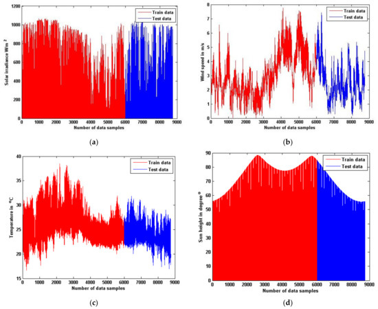
Figure 1.
Training and testing sample dataset of environmental parameters: (a) Solar radiation; (b) Wind speed; (c) Ambient temperature of the location; (d) Sun elevation.
The proposed methodology is about approximating the hourly data for daily and weekly forecasting. With the available hourly dataset, the authors tried to perform daily and weekly forecasting based on mathematical approximations. The corresponding approximation expressions are given in Equations (1)–(7) of Section 2.1. Here, the forecasting is made by LSTM predictor and the LSTM parameters are optimally tuned by the proposed hybrid CSO-GWO optimization algorithm. The performance of neural network models is greatly influenced by the random initialization of learning parameters. So, in the proposed paper, the crow search optimization algorithm is hybridized with the grey wolf optimization algorithm. The hybrid CSO-GWO optimization algorithm is employed to tune the weight and bias coefficients of the LSTM model. The architecture of the proposed methodology is presented in Figure 2. During the training process, 5-fold cross-validation is performed, and all the three reservoirs of the hourly, daily, and weekly dataset are segregated into 5-fold data and trained in parallel. While four folds are employed for training, the remaining 1-fold is utilized for testing. So, at the end of the training process, the entire training dataset will be at least trained and tested once. This improves the training accuracy and learning ability of the model. During the training process, each unit is trained to handle missing data situations with the common resource sharing ability of parallel processing. The input data are then normalized by min-max normalization and fed into the proposed deep learning LSTM predictor model. The performance is simulated in MATLAB R2020b environment.
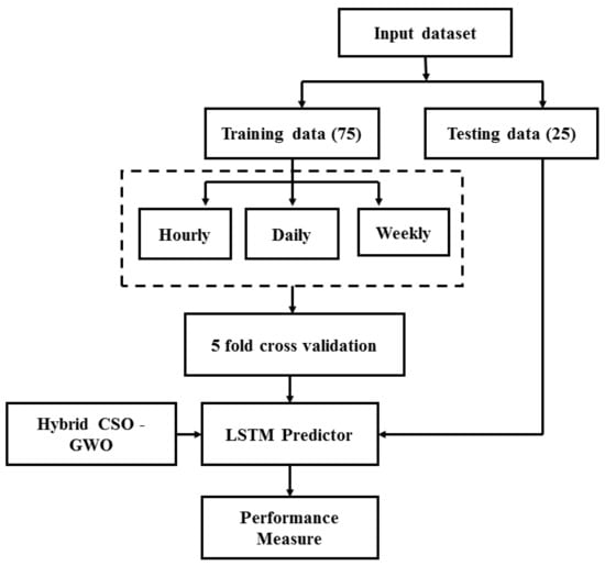
Figure 2.
The proposed methodology of the study.
2.1. Proposed Multi-Time Scale Forecasting
The single-stage forecasting will perform effectively for that specific period. It cannot be employed. Moreover, an effective forecasting resource sharing of various time scale data is helpful. For these reasons, a novel strategy to perform multi time scale anticipating is proposed to take focal points of relationships on various timescales. In the proposed solar irradiance forecasting model, the principal thought is to foresee the irradiance for various time scale with the available data. The timescale of each errand relies upon the availability of the irradiance data. For instance, the data employed for short term forecasting cannot be employed for long term forecasting. Whereas the developed model in this chapter with the irradiance data gathered in the hourly span can satisfy different undertakings of hour-ahead, day-ahead, and week ahead forecasting, the same cannot be made possible in a single-stage forecasting model because of insufficient data. In this investigation, two assignments with hourly and daily scale forecasting are made using the hourly irradiance information as in Figure 3.
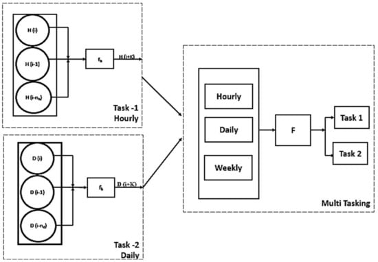
Figure 3.
Multi-tasking architecture.
The basic idea behind the proposed multi time scale solar irradiance forecasting is approximating hourly data corresponding to daily and weekly datasets by parallel processing resource sharing ability. The fundamental task here is to fill the missing data fields while the data are approximated to perform day ahead and week ahead forecasting. Instead of common data imputation strategy, the proposed model employed an autoregressive exogenous technique (ARX). Here, based on the linear combination of available past input and output samples, the specific system output is represented.
Based on the linear multi-input and multi-output autoregressive exogenous technique of Wu et al. [20], the proposed model is generalised as below:
where denote the number of a data sample of relative solar irradiance on different timescales, based on the history of data, while the relationship between the anticipated and the actual data is computed as coefficients , and is the error coefficient. are hourly, daily, and weekly solar irradiance that can be obtained as:
To improve the non-linear fitting ability, a deep LSTM based multi time scale forecasting model is established as:
2.2. Recurrent Neural Network
The learning mechanism employed to compute the new states recursively by applying activation functions over the inputs and the previous states of the network is termed recurrent neural networks (RNNs). It differs from conventional feed forward network by its feedback connectivity given to hidden units. The previous history of hidden states is stored in special storage units called context units, the stored data in the previous iteration will be utilized by the current iteration during training process. The special ability of RNN is to approximate the non-linear dynamics of system by dynamic mapping of input output sequences. The common learning methodology employed is gradient descent-based learning algorithm. The algorithm’s cost function is to reduce the error between the actual and predicted data, where the objective is to reduce the MSE between actual and predicted output.
A simple RNN architecture is depicted in Figure 4, where ,, represents the input, hidden, and output weights, respectively, and represents the delay unit. It is noted from the architecture that the feedback is not provided by the output connection from the output unit. Instead, the hidden unit undertakes it through a time shift operator. When the time shift operator is negative, then the node receives the input of content from the previous time interval. In contrast, in the case of a positive time shift, then it represents the input from future time interval. There exist various types of RNN networks, including Hopfield network, Elman network, Jordan network, long short-term neural network, echo state neural network, and so on. The common limitation of the RNN network is its gradient vanishing issue, so to address this issue, the LSTM neural network has been introduced which is employed to forecast the solar irradiance in this research contribution.
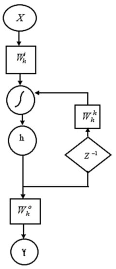
Figure 4.
Recurrent neural network architecture.
2.3. LSTM Deep Learning Model
The long short-term memory network is a kind of recurrent neural network, and the LSTM architecture handles the vanishing gradient problem of classic RNN. During the training process, the data flow is maintained by switching special gates that decide when to read, write, and what data to be stored in the gates coordinately. The deep LSTM architecture is presented in Figure 5, with the input gate , output gate , the forget gate and the context unit . The signal flow between the layers with long term learning dependencies is presented below:
where ,and are the weight and bias coefficients, while the operator is the element wise multiplication. The signal flow from one gate to another for a specific time instant is dependent on previous iteration state. For instance, the value to be stored in input gate is the output of the sigmoidal function employed over net input computed between the input and previous instances of hidden units. If the forget gate value is 1, the information in the memory cell is retained. Otherwise, it will be removed. The proposed LSTM model employs several stacked LSTM layers. The output of each layer is added linearly by employing the softmax activation function.
where is the output of a single LSTM shell.
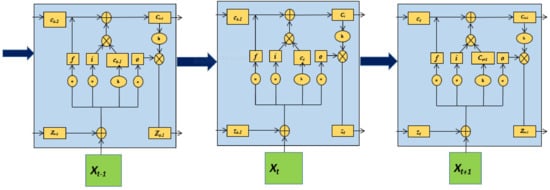
Figure 5.
LSTM deep learning model network layers.
The performance of neural networks models is greatly influenced by its random initialization of learning parameters. In this study, a hybrid optimization algorithm is developed to tune the model parameters to the optimal value. In swarm intelligence, not all the algorithms can perform similarly for all problem statements. Conventionally, they suffer from certain limitations, such as local stagnation issues, global stagnation issues, delayed convergence, and so on. To address these limitations, the algorithm should possess a better trade-off between its exploration and exploitation stability. Thus, in the proposed paper, a hybrid combination of crow search optimization algorithm (CSO) with grey wolf optimization algorithm (GWO) is made.
2.4. Chicken Swarm Optimization Algorithm—An Overview
Chick swarms’ hierarchical behaviour is inspired to propose an optimization scheme called the chicken swarm optimization algorithm. In this algorithm, the entire population is segregated into various groups. Among all groups, there will be a rooster and numerous hens and chicks. The fitness value decides the hierarchy of the swarms. The chicken learns from their experience instead of learning through experiment. The roosters guide the movement of hens and chicks. They produce distinct sounds for their communications among the population, and there will be dominant and submissive hens among the population. The dominant will be near to the rooster, while others will stand further away. They demand battle if any other group members enter their boundary, sometimes stealing food from other boundaries. The position of chicks will be based on the position of their moms:
where is the Gaussian distribution with the mean value of 0 and represents the standard deviation; the zero deviation error is reduced by , and is employed to avoid the zero division error; the rooster index is represented by k, and f is the fitness function value for the corresponding particle in the population. The position updating equation of hen is presented as follows:
where R is the uniform random number, the index of the rooster is shown by r1, and r2 is the index of chicken that is randomly selected from the population, such that r1 is not the same as that of r2. The chicks will follow the hen for food based on the following equation:
where FL is a parameter randomly chosen between 0 and 2. stands for the position of the mother hen in the population.
2.5. Grey Wolf Optimizer Algorithm—An Overview
The grey wolf optimizer is developed based on wolves’ hunting behaviour, the hierarchical behaviour of wolves and their social hunting mechanism is adopted to frame the algorithm. There exist four degrees of authority among wolves. The pioneer wolves that occupy the highest position of the hierarchy are the alpha wolves. They are the main decision-makers of the population and they drive the whole gathering. This wolf is the most dominant in the population. The population that follows the next hierarchy of dominant wolves is the beta wolf, and they will help the alpha in decision making and organizing the gathering. The third position involved is the omega wolves. These wolves are generally most fragile among the gathering and are in every case less allowed to eat and overwhelmed by all other predominant individuals from the gathering. The wolves that are not categorized according to these three classifications are the delta wolves. They are dominated by the first two hierarchical groups and tend to dominate the omega wolves. The entire population is highly organized for social hunting, and their prey encircling mechanism is mathematically expressed as follows:
The hunting process is mathematically written as
where is a coefficient vector that is a randomly generated value in the range of 2 to 0. For the wolves will attack the prey, and for the members are forced to move away from the prey.
2.6. Proposed Hybrid CSO-GWO Optimization Algorithm
The major issue faced by the swarm intelligence algorithms is the lack of a better trade-off between exploration and exploitation ability of the algorithm. The exploration ability defines the global search ability of the population. The prey identification process of an individual in the population is the exploration ability. Once the prey is identified, the entire population is coordinated to enjoy the food through exploitation. The population-based algorithms suffer from premature convergence, delayed convergence, local stagnation issue, local optimal and global optimal trapping issues, etc. In the proposed model, two algorithms are hybridized. The CSO optimizer is good at its exploration ability, and the GWO is good at its local hunting mechanism. Moreover, both the algorithms have the similarity of a three-layer hierarchy in terms of their social behaviour.
The Pseudocode of the proposed algorithm is presented in Algorithm 1, and the flow diagram is presented in Figure 6. The steps involved are presented as follows:
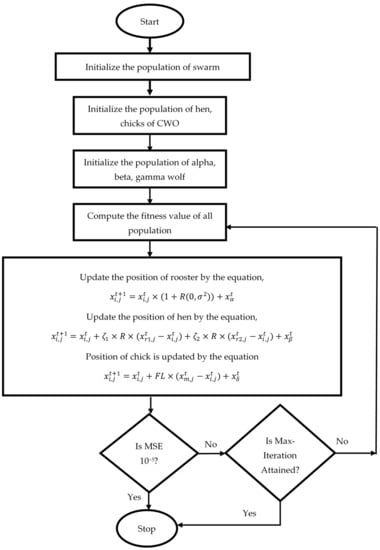
Figure 6.
Flow diagram of the proposed hybrid CSO-GWO algorithm.
The mathematical expressions depicting the movement of a rooster guided by alpha wolves are presented as follows:
| Algorithm 1 Proposed hybrid CSO-GWO optimizer |
| 1: Initialize the population of rooster, hen and chicks of CSO 2: Initialize the population of alpha, beta, delta wolves of GWO 3: Initialize r1, r2, FL, R(.), a 4: while (MSE = 10–5 || Max_iter = 700) 5: { 6: for all individual in population 7: { 8: do 9: Evaluate the fitness value of all swarm in the population 10: Update the position of , and wolves in the population is updated as 11: 12: 13: 14: Update position of rooster, hen and chick as, 15: 16: 17: 18: } 19: end for 20: } 21: end while 22: return the evaluated fitness value 23: return the iter_no 24: return MSE |
The position updating equation of hen guided by beta wolves is presented as follows:
Delta wolves guide the position of chick based on the following equation,
- Step 1: The population of rooster, hen, and the chicks of CSO algorithm are initialized.
- Step 2: The population of alpha, beta and delta wolves of the grey wolf optimization algorithm is initialized.
- Step 3: Until stopping criteria is attained, the fitness function is evaluated for the entire population. Based on the fitness value obtained, the position of chicks and hens are updated.
- Step 4: Steps 2 to 4 is repeated until the stopping criteria of the maximum number of iterations or minimum MSE order of 10−5 are attained.
- Step 5: The fitness value and the corresponding MSE is returned.
The model is made to run until error convergence of 10−5, the mean square error between actual and predicted data is made as to the fitness function. The entire dataset is approximated into three records: hourly, daily, and weekly. Three LSTM models are developed. Three reservoirs of datasets train each, the forecasted data of each LSTM unit is linearly combined at the output layer by a SoftMax activation function. The number of hidden layers is fixed after 25 trial runs, and the number of hidden units at each layer is fixed by the trial-and-error method based on the thumb rule, with the number of hidden layers of 4, 3, and 5 for each LSTM layer, respectively. For each trial run, the model is evaluated for training and testing accuracy. The number of hidden layers and hidden neurons are fixed such that the model is free from over and under fitting issues.
During the training process, 5-fold cross-validation is performed. All the three reservoirs of hourly, daily and weekly dataset are segregated into 5-fold data and trained in parallel. While four folds are employed for training, the remaining 1-fold is utilized for testing. So, at the end of training process the entire training dataset will be at least trained and tested for once. This improves the training accuracy and learning ability of the model. During the training process, each unit is trained to handle missing data situations with the common resource sharing ability of parallel processing. The final output of the model is the linear combination of each LSTM unit. The proposed model’s performance is validated by investigating the model response for hourly, daily, and weekly prediction based on training the model with the hourly dataset. The forecasted result of three-time scale forecasting is mapped with the actual dataset and presented in Figure 7, Figure 8 and Figure 9 for hourly, daily, and weekly irradiance forecasting, respectively.
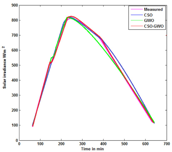
Figure 7.
Hourly prediction of solar irradiance using CSO, GWO, and hybrid CSO-GWO with LSTM predictor for 8 October 2020.
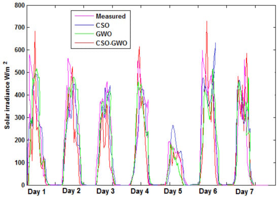
Figure 8.
Daily prediction of solar irradiance using CSO, GWO, and hybrid CSO-GWO with LSTM predictor for seven days of 1st week of November 2020.
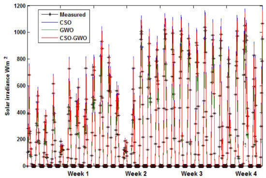
Figure 9.
Weekly prediction of solar irradiance using CSO, GWO, and hybrid CSO-GWO with LSTM predictor for the weeks of December 2020.
The proposed multi scale solar radiation forecasting performs three-time scale forecasting such as hourly, daily and weekly forecasting on the basis of hourly data set with better resource sharing ability. The proposed deep learning LSTM model parameters are optimally tuned by the proposed hybrid CSO-GWO optimization algorithm, which also optimally tunes the network parameters such as weight and bias coefficients. The input data are normalized by min-max normalization and fed into the proposed deep learning LSTM predictor model. The performance is simulated in MATLAB R2014a environment and executed in Intel Duo Core2 processor with 2 GB RAM of speed, 2.27 GHz.
The performance metrics employed to evaluate the performance of the model are presented as follows:
Mean square error (MSE): The mean value of deviation between the actual and predicted MSE depicts data. Here, the large error values are highlighted.
Mean absolute percentage error (MAPE): A common methodology employed in statistics to the measure the level of error that occurs in prediction.
Direct accuracy (DA): The direct prediction accuracy of the forecasted series is demonstrated by DA and expressed as follows:
where n is the number of data samples, is actual data, is the predicted output.
Since the proposed model has stochastic parameters, statistical analysis shows that the obtained results are not affected by randomness. Pearson’s test and coefficient of determination were obtained to signify the statistical analysis of the proposed regression model, and the Pearson correlation is presented as follows:
where and are the means of actual and predicted data, respectively.
When the coefficient of determination (R2) and the correlation value (r) approaches near 1, then the proposed model can be validated as statistically fit to perform solar irradiance forecasting.
3. Results
The model is evaluated for individual time scale forecasting and compared with the proposed multi-time scale forecasting performance, as presented in Table 2. To investigate the extent to which the multi scale approximation results deviated from individual time scale results, here, for individual time scale forecasting, the model is trained with hourly data for hourly forecasting, daily irradiance data for daily forecasting, and weekly data for weekly forecasting. The proposed model is compared with the multi time scale forecasting model of Wu et al. [34] for both single-stage and multi time scale forecasting, to demonstrate the significance of the proposed strategy based on the performance metric results, such as MSE (mean square error), MAPE (mean absolute percentage error), and DA (direct accuracy). The performance of the multi time scale model for hourly, daily, and weekly forecasting is shown in Figure 7, Figure 8 and Figure 9. The figures are plotted for the testing dataset. In this study, January–September monthly data are employed as the training dataset and October–December monthly data are forecasted as the testing response. Figure 7 depicts the prediction response for 8 October 2020, it shows the hourly forecasting performance. Figure 8 shows the performance of daily time scale forecasting, and it is illustrated for seven days of the first week of November. Figure 9 depicts the performance of weekly time scale forecasting. This plot is made for the weeks of December.
Table 2.
The performance metric results of the proposed models.
Investigating the performance of the proposed multistage solar irradiance forecasting, the following inferences are made:
The LSTM is employed for single scale and multi scale solar irradiance forecasting. For individual time scale forecasting for hourly time scale, the obtained MSE is 0.3670 W/m2, the MAPE is 0.1249 and the DA is 0.1398 as in Table 2. In contrast, employing LSTM for multi time scale forecasting, the reported MSE is 0.2392 W/m2, the MAPE is 0.3562 and DA is 0.3189. For day ahead forecasting, the MSE, MAPE, and DA of multi time scale forecasting is 0.4326, 0.4652, and 0.4206, respectively. The same for individual time scale forecasting is 0.3468, 0.3135, and 0.3428, respectively. For week ahead forecasting, the performance metric values for multi time scale forecasting is 0.3456, 0.5521, and 0.5735, respectively, for MSE, MAPE, and DA. Similarly, for individual time scale forecasting, the reported metric results are 0.4021, 0.4350, and 0.2353, respectively. Here, it is observed that the performance of LSTM for multi time scale forecasting does not greatly deviate from individual time scale forecasting, whereas the impact of multi scale approximation is reflected in metric results as well. In Figure 8, daily solar radiation is predicted, showing that day 5 is cloudy, which shows that the error is less in the daily prediction curves in the proposed algorithm CSO, GWO, and hybrid CSO-GWO algorithm.
3.1. Performance of CSO Algorithm
The model parameters of the proposed LSTM are optimally tuned by CSO algorithm in Figure 7, Figure 8 and Figure 9. In comparison with the classic LSTM model, the CSO-LSTM performance metric results are improved. The multi time scale forecasting results of CSO-LSTM demonstrate 3% better MSE value than that of conventional LSTM for hourly time scale. The MAPE and DA is improved to the percentage of 12.5% and 5.17% better than that of conventional LSTM. Similarly, for individual time scale forecasting, the performance of CSO-LSTM is 11.09% and MAPE is improved to 18.08% and the DA is improved to 22.93% for hourly time scale forecasting. For day ahead forecasting, the proposed CSO-LSTM has shown improved performance of 8% MSE, 7.2% MAPE, and 10.5% DA. For individual time scale forecasting, the performance is improved to the value of 10.17% MSE, 19.1% MAPE value, and 22.9% DA value. For weekly solar radiation forecasting, the MSE value is 2% higher than that of conventional LSTM, while the MAPE and DA is improved to 14.99% and 25% respectively for multi time scale forecasting. The individual reported better performance of 30% better MSE, 20% better MAPE, and the DA has better result of 10%.
3.2. Performance of GWO Optimization Algorithm
The LSTM model is optimally tuned by GWO optimization algorithm in Figure 7, Figure 8 and Figure 9, with reported 23.41% of improved MSE, 35.2% of MAPE, and 16.87% of DA than the conventional LSTM model for multi-scale hourly forecasting. Similarly, for individual prediction, 30%, 8.6%, and 4.6% of MSE, MAPE, and DA were reported respectively. For daily time scale, the multi time scale forecasting attained an improved MSE of 37.1%, 21.31% MAPE, and 25.13% better DA, respectively. For the individual time scale, it is found to be 28.27% of MSE, 20.6% of MAPE, and 20.8% of DA, respectively. For weekly time scale forecasting, the MSE value is 14.37% better than that of conventional model, 30.79% of MAPE and 29.89% of DA for multi time scale forecasting. For the individual time scale, the improved performance is 31% of MSE, 33.2% of MAPE, and 13% of DA, respectively.
3.3. Performance of Hybrid CSO-GWO Optimization Algorithm
On hybridizing the CSO and GWO LSTM model in Figure 7, Figure 8 and Figure 9, there has been reported a significant improvement in performance metric results. For hourly time scale forecasting, the multi scale model reported 23.88% better MSE, 32.52% of MAPE, and 31.62% of DA, respectively. Similarly for individual forecasting, the obtained results are 36.66% better MSE, 7.6% improved MAPE, and 12% of DA, respectively. For daily forecasting the multi scale model reported 38.05% better MSE, 30.7% of MAPE and 37.36% of DA respectively than the conventional LSTM. For individual forecasting the weekly forecasting has improved metric results of 34.47% better MSE, 24.21% better MAPE, and 27.94% better DA, respectively. The result is analysed for weekly time scale forecasting, the MSE is 24.38% improved than that of conventional LSTM and the MAPE and DA is 15% and 45.65% respectively. The same for individual time scale forecasting is 39.71% better MSE, the MAPE is 24.99% improved, and DA is 21.34% better than that of the conventional LSTM model.
In the above results, it is observed that for both individual and multi time scale forecasting the performance of classic LSTM model is improved by introducing CSO and GWO optimization algorithm. On introducing hybrid CSO-GWO optimization, the performance for both time scale models is considerably improved. Though the performance of the conventional LSTM for multi timescale forecasting is not up to the level of individual forecasting, the hybrid CSO-GWO based LSTM model results for multi time scale forecasting are significantly improved compared with the conventional LSTM model for single time scale forecasting. Thus, the lacuna encountered in first point of this discussion is encountered here, whereby on introducing hybrid CSO-GWO, the impact of multi time scale approximation is well-adjusted and the performance is greatly improved.
3.4. Comparative Analysis with Existing Works of Literature
The performance of the proposed multi scale solar irradiance forecasting is compared with the existing works of literature such as ESO [34], PSO-SVR [47], and GRU [50]. For hourly time scale forecasting, the performance of the proposed hybrid CSO-GWO LSTM model has reported 3.99% improved MSE, 5.05% of MAPE and 6.31% of better DA value than the ESO neural network strategy. On comparing with PSO-SVR, the proposed strategy outperformed with 20.2% better MSE, 38.32% of MAPE and 38.54% better DA value, respectively. On comparing with the GRU, the proposed strategy outperformed with 32.4% of MSE, 24.1% better MAPE, and 15.9% better DA. For daily time scale forecasting, the performance of the proposed models reported 9.10% better MSE than ESO neural network, 3.87% of better MAPE, and 4.58% better DA results, respectively. On comparing with PSO-SVR, the proposed strategy reported 24.3% better MSE, 33.8% better MAPE, and 42.7% better DA value respectively. Similarly, on comparing with GRU the proposed strategy reported 9.31% better MSE, 11.01% better MAPE and 10.92% improved DA respectively. For weekly time scale forecasting, the performance of the proposed scheme has reported improved performance of 12.6% better MSE, 32.7% better MAPE and 15.21% better DA results than the ESO technique. On comparing with PSO-SVR strategy, the performance of the proposed model has 31.96% better MSE, 32.71% better MAPE, and 30.01% better DA, respectively. Similarly, on comparing with GRU, the proposed model reported 38.78% better MSE, 29.72% better MAPE, and 24.58% better DA, respectively.
For multi-time scale forecasting, the proposed strategy has shown enhanced performance of 5.75% better MSE, 21.9% better MAPE, and 5.05% better DA than the ESO for hourly time scale forecasting, in comparison with PSO-SVR the proposed technique outperformed with 16.9% better MSE, 38% improved MAPE, 23.6% better DA, respectively. Similarly, the proposed model outperformed GRU model with improved metric results of 12.9% better MSE, 17.4% better MAPE, and 25.6% better DA, respectively. For daily time scale forecasting, the proposed model outperformed the ESO with 24.0% better MSE, 16.4% better MAPE and 54.9% better 14.9% better DA respectively. On comparing with PSO-SVR the performance of the proposed strategy has 15.2% better MSE, 37.9% better MAPE, and 25.5% better DA, respectively. On comparing with GRU the performance of the proposed technique is 25.2% better MSE, 37.9% better MAPE, 25.5% better DA, respectively. For weekly forecasting, the performance of the proposed model is 23.01% better MSE than ESO strategy, 21.42% of MAPE, and 39.22% better DA, respectively. On comparing with PSO-SVR the performance of the proposed model has 21.82% better MSE, 38.58% better MAPE and 47.82% better DA, respectively. In comparison with the GRU model, the proposed strategy has shown performance of 13.23% better MSE, 13% better MAPE, and 30.41% better DA, respectively.
The convergence of the proposed optimization algorithm towards stopping condition is depicted in Figure 10. Over the iterations, the models trains deeply so the error starts to decrease and converges towards the attainment of optimal solution. The graph shows good convergence of a measure, as the curve becomes asymptotic and plots values for the final. On comparing with CSO and GWO, the proposed hybrid CSO-GWO converges fast demonstrating the less computational time. The proposed multi time scale model demonstrated that it could outperform individual time scale forecasting with the particular time scale training dataset. Moreover, it illustrated significant improvement in forecasting accuracy on multi time scale forecasting with a training dataset on an hourly basis. The proposed hybrid CSO-GWO based LSTM model’s performance outperformed the other models, including the LSTM strategy, the LSTM model tuned by the CSO, and GWO individually.
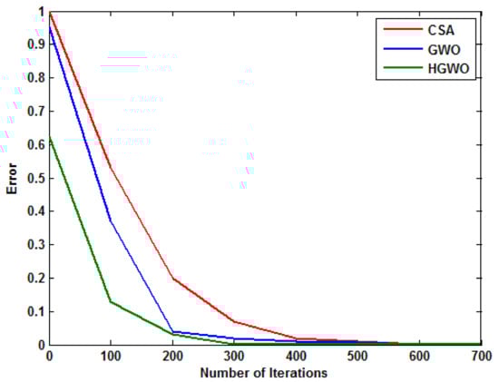
Figure 10.
Error convergence of the proposed algorithms.
Based on the statistical score obtained from the proposed model, it is clearly demonstrated that the proposed hybrid CSO-GWO-LSTM model is not affected by the algorithm’s stochastic factors, and it is found to be statistically fit, as shown in Table 3.
Table 3.
Statistical Analysis of the Proposed Model.
The proposed model addressed the scenario of various timescale forecasting with the available dataset. The long-term forecasting cannot be made with the short-term dataset by the conventional models in the existing literature. In this model, seasonal wise forecasting has not been performed. Future work is recommended for multi-seasonal forecasting based on the proposed study for solar radiation forecasting.
4. Conclusions
In this chapter, a multi-time scale solar irradiance forecasting strategy is presented. An LSTM-based deep recurrent neural network architecture is developed, and the proposed CSO-GWO optimizer algorithm optimally tunes the model parameters. The model is trained with an hourly solar irradiance dataset, and the forecasting is made with hourly, daily, and weekly-based forecasting with resource sharing ability. The model is evaluated with performance metrics such as MSE (mean square error), MAPE (mean absolute percentage error), DA (direct accuracy), and to signify the obtained performance is not affected by the algorithm’s stochastic parameters, a statistical analysis is undertaken. The proposed model outperformed others with better metric results for single time scale forecasting and multi time scale forecasting with better metric results. In comparison with the hourly results of the CSO, GWO, and CSO-GWO LSTM based models, the proposed model gives the minimal error in the performance metrics MSE (3.412 × 10⁻⁴), MAPE (0.0310), and DA (2.71 × 10⁻³). Similarly, for daily and weekly MSE (5.208 × 10⁻²), MAPE (0.1582), and DA (0.0470), and to signify the obtained performance is not affected by the algorithm’s stochastic parameters, a statistical analysis is undertaken. The proposed model outperformed with better metric results for single time scale forecasting and multi time scale forecasting with better metric results.
Author Contributions
Conceptualization, N.Y.J. and I.B.; methodology, R.S. and A.K.; software, A.G., A.K. and B.S.; validation, R.R., N.Y.J., R.S. and U.S.; formal analysis, N.Y.J. and B.S.; investigation, I.B. and A.K.; resources, A.G. and N.Y.J.; data curation, U.S.; writing—original draft preparation, R.S., R.R. and B.S.; writing—review and editing, U.S. and A.G.; visualization, A.G. and U.S.; supervision, I.B. and A.K.; project administration, A.K., N.Y.J. and U.S.; funding acquisition, A.G. and U.S. All authors have read and agreed to the published version of the manuscript.
Funding
The Article Processing Charge was funded by Prince Sultan University.
Institutional Review Board Statement
Not applicable.
Data Availability Statement
All the data is included in the manuscript.
Acknowledgments
The authors would also like to acknowledge Renewable Energy Lab, College of Engineering, Prince Sultan University for technical support in this article. The authors would like to acknowledge the support of Prince Sultan University for paying the Article Processing Charge (APC) of this publication.
Conflicts of Interest
The authors declare no conflict of interest.
References
- Gielen, D.; Boshell, F.; Saygin, D.; Bazilian, M.D.; Wagner, N.; Gorini, R. The role of renewable energy in the global energy transformation. Energy Strategy Rev. 2019, 24, 38–50. [Google Scholar] [CrossRef]
- Kabir, E.; Kumar, P.; Kumar, S.; Adelodun, A.A.; Kim, K.H. Solar energy: Potential and future prospects. Renew. Sustain. Energy Rev 2018, 82, 894–900. [Google Scholar] [CrossRef]
- Shahsavari, A.; Akbari, M. Potential of solar energy in developing countries for reducing energy-related emissions. Renew. Sustain. Energy Rev. 2018, 90, 275–291. [Google Scholar] [CrossRef]
- Hosseini, S.E.; Wahid, M.A. Hydrogen from solar energy, a clean energy carrier from a sustainable source of energy. Int. J. Energy Res. 2020, 44, 4110–4131. [Google Scholar] [CrossRef]
- Khalid, M.; Shanks, K.; Ghosh, A.; Tahir, A.; Sundaram, S.; Mallick, T.K. Temperature regulation of concentrating photovoltaic window using argon gas and polymer dispersed liquid crystal fi lms. Renew. Energy 2021, 164, 96–108. [Google Scholar] [CrossRef]
- Mesloub, A.; Ghosh, A.; Albaqawy, G.A.; Noaime, E.; Alsolami, B.M. Energy and Daylighting Evaluation of Integrated Semitransparent Photovoltaic Windows with Internal Light Shelves in Open-Office Buildings. Adv. Civ. Eng. 2020, 2020. [Google Scholar] [CrossRef]
- Alrashidi, H.; Issa, W.; Sellami, N.; Ghosh, A.; Mallick, T.K.; Sundaram, S. Performance assessment of cadmium telluride-based semi-transparent glazing for power saving in façade buildings. Energy Build. 2020, 215, 109585. [Google Scholar] [CrossRef]
- Karthick, A.; Kalidasa Murugavel, K.; Ghosh, A.; Sudhakar, K.; Ramanan, P. Investigation of a binary eutectic mixture of phase change material for building integrated photovoltaic (BIPV) system. Sol. Energy Mater. Sol. Cells 2020, 207. [Google Scholar] [CrossRef]
- Ramanan, P.; Kalidasa Murugavel, K.; Karthick, A. Performance analysis and energy metrics of grid-connected photovoltaic systems. Energy Sustain. Dev. 2019, 52, 104–115. [Google Scholar] [CrossRef]
- Pichandi, R.; Murugavel Kulandaivelu, K.; Alagar, K.; Dhevaguru, H.K.; Ganesamoorthy, S. Performance enhancement of photovoltaic module by integrating eutectic inorganic phase change material. Energy Sources Part A Recover. Util. Environ. Eff. 2020. [Google Scholar] [CrossRef]
- Ghosh, A.; Norton, B.; Mallick, T.K. Influence of atmospheric clearness on PDLC switchable glazing transmission. Renew. Energy 2018, 172, 257–264. [Google Scholar] [CrossRef]
- Ghosh, A.; Norton, B. Optimization of PV powered SPD switchable glazing to minimise probability of loss of power supply. Renew. Energy 2019, 131, 993–1001. [Google Scholar] [CrossRef]
- Mesloub, A.; Ghosh, A. Daylighting performance of light shelf photovoltaics (LSPV) for office buildings in hot desert-like regions. Appl. Sci. 2020, 10, 7959. [Google Scholar] [CrossRef]
- Miller, S.D.; Rogers, M.A.; Haynes, J.M.; Sengupta, M.; Heidinger, A.K. Short-term solar irradiance forecasting via satellite/model coupling. Sol. Energy 2018, 168, 102–117. [Google Scholar] [CrossRef]
- Diagne, M.; David, M.; Lauret, P.; Boland, J.; Schmutz, N. Review of solar irradiance forecasting methods and a proposition for small-scale insular grids. Renew. Sustain. Energy Rev. 2013, 27, 65–76. [Google Scholar] [CrossRef]
- Akarslan, E.; Hocaoglu, F.O. A novel method based on similarity for hourly solar irradiance forecasting. Renew. Energy 2017, 112, 337–346. [Google Scholar] [CrossRef]
- Zeng, X.; Hammid, A.T.; Kumar, N.M.; Subramaniam, U.; Almakhles, D.J. A grasshopper optimization algorithm for optimal short-term hydrothermal scheduling. Energy Rep. 2021, 7, 314–323. [Google Scholar] [CrossRef]
- Akarslan, E.; Hocaoglu, F.O.; Edizkan, R. Novel short term solar irradiance forecasting models. Renew. Energy 2018, 123, 58–66. [Google Scholar] [CrossRef]
- Balasubramanian, K.; Thanikanti, S.B.; Subramaniam, U.N.; Sudhakar, N.; Sichilalu, S. A novel review on optimization techniques used in wind farm modelling. Renew. Energy Focus 2020, 35, 84–96. [Google Scholar] [CrossRef]
- Marzouq, M.; El Fadili, H.; Zenkouar, K.; Lakhliai, Z.; Amouzg, M. Short term solar irradiance forecasting via a novel evolutionary multi-model framework and performance assessment for sites with no solar irradiance data. Renew. Energy 2020, 157, 214–231. [Google Scholar] [CrossRef]
- Yin, W.; Han, Y.; Zhou, H.; Ma, M.; Li, L.; Zhu, H. A novel non-iterative correction method for short-term photovoltaic power forecasting. Renew. Energy 2020, 159, 23–32. [Google Scholar] [CrossRef]
- Madurai Elavarasan, R.; Afridhis, S.; Vijayaraghavan, R.R.; Subramaniam, U.; Nurunnabi, M. SWOT analysis: A framework for comprehensive evaluation of drivers and barriers for renewable energy development in significant countries. Energy Rep. 2020, 6, 1838–1864. [Google Scholar] [CrossRef]
- Dong, N.; Chang, J.F.; Wu, A.G.; Gao, Z.K. A novel convolutional neural network framework based solar irradiance prediction method. Int. J. Electr. Power Energy Syst. 2020, 114. [Google Scholar] [CrossRef]
- Yan, K.; Shen, H.; Wang, L.; Zhou, H.; Xu, M.; Mo, Y. Short-term solar irradiance forecasting based on a hybrid deep learning methodology. Information 2020, 11, 32. [Google Scholar] [CrossRef]
- Mahmoudimehr, J.; Sebghati, P. A novel multi-objective Dynamic Programming optimization method: Performance management of a solar thermal power plant as a case study. Energy 2019, 168, 796–814. [Google Scholar] [CrossRef]
- Lotfi, M.; Javadi, M.; Osório, G.J.; Monteiro, C.; Catalão, J.P.S. A novel ensemble algorithm for solar power forecasting based on kernel density estimation. Energies 2020, 13, 216. [Google Scholar] [CrossRef]
- Zang, H.; Liu, L.; Sun, L.; Cheng, L.; Wei, Z.; Sun, G. Short-term global horizontal irradiance forecasting based on a hybrid CNN-LSTM model with spatiotemporal correlations. Renew. Energy 2020, 160, 26–41. [Google Scholar] [CrossRef]
- Lee, D.; Kim, K. Recurrent neural network-based hourly prediction of photovoltaic power output using meteorological information. Energies 2019, 12, 215. [Google Scholar] [CrossRef]
- Cheng, L.; Zang, H.; Ding, T.; Sun, R.; Wang, M.; Wei, Z.; Sun, G. Ensemble recurrent neural network based probabilistic wind speed forecasting approach. Energies 2018, 11, 958. [Google Scholar] [CrossRef]
- Wang, Y.; Liao, W.; Chang, Y. Gated recurrent unit network-based short-term photovoltaic forecasting. Energies 2018, 11, 2163. [Google Scholar] [CrossRef]
- Wen, L.; Zhou, K.; Yang, S.; Lu, X. Optimal load dispatch of community microgrid with deep learning based solar power and load forecasting. Energy 2019, 171, 1053–1065. [Google Scholar] [CrossRef]
- Li, G.; Wang, H.; Zhang, S.; Xin, J.; Liu, H. Recurrent neural networks based photovoltaic power forecasting approach. Energies 2019, 12, 2538. [Google Scholar] [CrossRef]
- Husein, M.; Chung, I.Y. Day-ahead solar irradiance forecasting for microgrids using a long short-term memory recurrent neural network: A deep learning approach. Energies 2019, 12, 1856. [Google Scholar] [CrossRef]
- Di Piazza, A.; Di Piazza, M.C.; La Tona, G.; Luna, M. An artificial neural network-based forecasting model of energy-related time series for electrical grid management. Math. Comput. Simul. 2021, 184, 294–305. [Google Scholar] [CrossRef]
- Jung, Y.; Jung, J.; Kim, B.; Han, S.U. Long short-term memory recurrent neural network for modeling temporal patterns in long-term power forecasting for solar PV facilities: Case study of South Korea. J. Clean. Prod. 2020, 250, 119476. [Google Scholar] [CrossRef]
- Wu, Z.; Li, Q.; Xia, X. Multi-timescale Forecast of Solar Irradiance Based on Multi-task Learning and Echo State Network Approaches. IEEE Trans. Ind. Inform. 2021, 17, 300–310. [Google Scholar] [CrossRef]
- Wang, F.; Yu, Y.; Zhang, Z.; Li, J.; Zhen, Z.; Li, K. Wavelet decomposition and convolutional LSTM networks based improved deep learning model for solar irradiance forecasting. Appl. Sci. 2018, 8, 1286. [Google Scholar] [CrossRef]
- Qing, X.; Niu, Y. Hourly day-ahead solar irradiance prediction using weather forecasts by LSTM. Energy 2018, 148, 461–468. [Google Scholar] [CrossRef]
- Li, J.; Ward, J.K.; Tong, J.; Collins, L.; Platt, G. Machine learning for solar irradiance forecasting of photovoltaic system. Renew. Energy 2016, 90, 542–553. [Google Scholar] [CrossRef]
- Alzahrani, A.; Shamsi, P.; Dagli, C.; Ferdowsi, M. Solar Irradiance Forecasting Using Deep Neural Networks. Procedia Comput. Sci. 2017, 114, 304–313. [Google Scholar] [CrossRef]
- Siddiqui, T.A.; Bharadwaj, S.; Kalyanaraman, S. A deep learning approach to solar-irradiance forecasting in sky-videos. In Proceedings of the 2019 IEEE Winter Conference on Applications of Computer Vision (WACV), Waikoloa, HI, USA, 7–11 January 2019; pp. 2166–2174. [Google Scholar] [CrossRef]
- Khodayar, M.; Mohammadi, S.; Khodayar, M.E.; Wang, J.; Liu, G. Convolutional graph autoencoder: A generative deep neural network for probabilistic spatio-temporal solar irradiance forecasting. IEEE Trans. Sustain. Energy 2020, 11, 571–583. [Google Scholar] [CrossRef]
- Sharma, A.; Kakkar, A. Forecasting daily global solar irradiance generation using machine learning. Renew. Sustain. Energy Rev. 2018, 82, 2254–2269. [Google Scholar] [CrossRef]
- Ssekulima, E.B.; Anwar, M.B.; Al Hinai, A.; El Moursi, M.S. Wind speed and solar irradiance forecasting techniques for enhanced renewable energy integration with the grid: A review. IET Renew. Power Gener. 2016, 10, 885–898. [Google Scholar] [CrossRef]
- Wang, W.; Zhen, Z.; Li, K.; Lv, K.; Wang, F. An Ultra-short-term Forecasting Model for High-resolution Solar Irradiance Based on SOM and Deep Learning Algorithm. In Proceedings of the 2019 IEEE Sustainable Power and Energy Conference (iSPEC), Beijing, China, 21–23 November 2019; pp. 1090–1095. [Google Scholar] [CrossRef]
- Dong, Z.; Yang, D.; Reindl, T.; Walsh, W.M. A novel hybrid approach based on self-organizing maps, support vector regression and particle swarm optimization to forecast solar irradiance. Energy 2015, 82, 570–577. [Google Scholar] [CrossRef]
- Wojtkiewicz, J.; Katragadda, S.; Gottumukkala, R. A Concept-Drift Based Predictive-Analytics Framework: Application for Real-Time Solar Irradiance Forecasting. In Proceedings of the 2018 IEEE International Conference on Big Data (Big Data), Seattle, WA, USA, 10–13 December 2019; pp. 5462–5464. [Google Scholar] [CrossRef]
- Wang, F.; Zhen, Z.; Liu, C.; Mi, Z.; Shafie-Khah, M.; Catalão, J.P.S. Time-section fusion pattern classification based day-ahead solar irradiance ensemble forecasting model using mutual iterative optimization. Energies 2018, 11, 184. [Google Scholar] [CrossRef]
- Peng, Z.; Peng, S.; Fu, L.; Lu, B.; Tang, J.; Wang, K.; Li, W. A novel deep learning ensemble model with data denoising for short-term wind speed forecasting. Energy Convers. Manag. 2020, 207, 112524. [Google Scholar] [CrossRef]
- Kartini, U.T.; Chen, C.R. Short Term Forecasting of Global Solar Irradiance by k-Nearest Neighbor Multilayer Backpropagation Learning Neural Network Algorithm. In Proceedings of the International Conference on Graphics and Signal Processing (ICGSP ’17), Singapore, Singapore, 24–27 June 2017; Association for Computing Machinery: New York, NY, USA, 2017; pp. 96–100. [Google Scholar] [CrossRef]
- Ren, Y.; Suganthan, P.N.; Srikanth, N. Ensemble methods for wind and solar power forecasting—A state-of-the-art review. Renew. Sustain. Energy Rev. 2015, 50, 82–91. [Google Scholar] [CrossRef]
- Aryaputera, A.W.; Yang, D.; Walsh, W.M. Day-Ahead Solar Irradiance Forecasting in a Tropical Environment. J. Sol. Energy Eng. Trans. ASME 2015, 137, 1–7. [Google Scholar] [CrossRef]
- Melzi, F.N.; Touati, T.; Same, A.; Oukhellou, L. Hourly solar irradiance forecasting based on machine learning models. In Proceedings of the 2016 15th IEEE International Conference on Machine Learning and Applications (ICMLA), Anaheim, CA, USA, 18–20 December 2017; pp. 441–446. [Google Scholar] [CrossRef]
- Rajagukguk, R.A.; Ramadhan, R.A.; Lee, H.J. A Review on Deep Learning Models for Forecasting Time Series Data of Solar Irradiance and Photovoltaic Power. Energies 2020, 13, 6623. [Google Scholar] [CrossRef]
- Photovoltaic Geographical Information System. Available online: https://re.jrc.ec.europa.eu/pvg_tools/en/#MR (accessed on 4 December 2020).
Publisher’s Note: MDPI stays neutral with regard to jurisdictional claims in published maps and institutional affiliations. |
© 2021 by the authors. Licensee MDPI, Basel, Switzerland. This article is an open access article distributed under the terms and conditions of the Creative Commons Attribution (CC BY) license (https://creativecommons.org/licenses/by/4.0/).