A Novel Feature Extraction Method for the Condition Monitoring of Bearings

Abstract

This paper presents an innovative approach to the extraction of an indicator for the monitoring of bearing degradation. This approach is based on the principles of the empirical mode decomposition (EMD) and the Hilbert transform (HT). The proposed approach extracts the temporal components of oscillating vibration signals called intrinsic mode functions (IMFs). These components are classified locally from the highest frequencies to the lowest frequencies. By selecting the appropriate components, it is possible to construct a bank of self-adaptive and automatic filters. Combined with the HT, the EMD allows an estimate of the instantaneous frequency of each IMF. A health indicator called the Hilbert marginal spectrum density is then extracted in order to detect and diagnose the degradation of bearings. This approach was validated on two test benches with variable speeds and loads. The obtained results demonstrated the effectiveness of this approach for the monitoring of ball and roller bearings.

1. Introduction to Bearings

Bearings are mechanical components used to provide a mobile connection between two rotating elements. This system increases the rotation speed while reducing the friction and the transmission of forces by replacing sliding with rotational motion. Bearings are therefore found where rotation is necessary (cars, electric motors, tools, etc.).

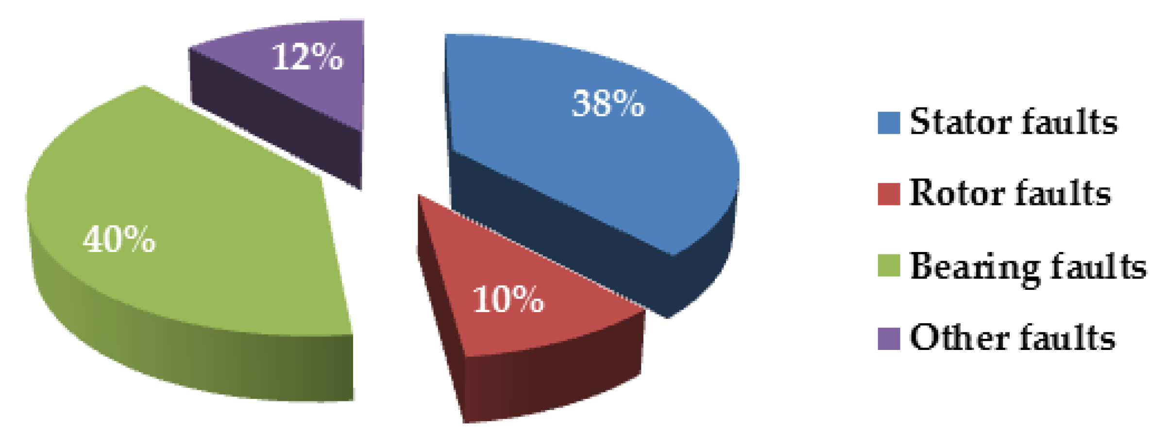
Studies conducted on induction motors have classified the most common fault mechanisms according to bearing faults, stator faults, rotor faults, and other faults (see Figure 1). These studies were carried out by the engine reliability group of the IEEE-Industry Applications Society (IAS), which studied 1141 motors, and the Electrical Energy Research Institute (EERI), which studied 6312 motors rated above 148 KW.

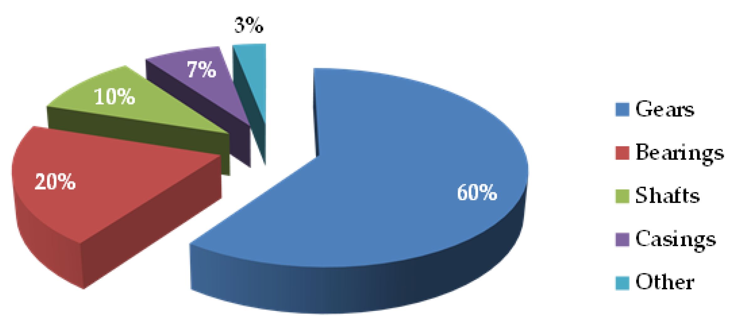
Additionally, as shown in Figure 2, studies dealing with faults located in power transmissions based on gearboxes have demonstrated that one of the most susceptible components to fail is a bearing [3]. Beyond manufacturing or assembly faults, the causes of damage are numerous and give rise to anomalies with several degrees of severity. It is therefore logical, from an industrial and scientific point of view, to focus diagnostic efforts mainly on bearings.

There exists in the literature a wide variety of signal processing tools used in bearing diagnostics. These methods can be classified into three categories based on one, two, and three dimensional indicators, respectively.

-

One-dimensional indicators

These methods are based on statistical indicators that quantify the information contained in the signals. Monitoring the evolution of these indicators provides more or less precise and complete information about the health of bearings. These indicators are mainly based on the calculation of the rms value, the crest factor, and kurtosis. The rms value was one of the first indicators used in the industry. Excessive variation in the rms level usually means a change in health status and therefore possible failure. One of the major drawbacks of using the rms is that it can give a late alarm, especially in the case of bearing faults where the variation in the signal due to the appearance of the fault is masked by other components of high amplitude (see Figure 21). The crest factor enables fault detection by measuring the ratio between the maximum value of the signal modulus (crest value) and its rms value. Other indicators have been developed based on the crest factor, such as the K-factor, by multiplying the peak value by the rms value or the peak-to-peak value, measuring the difference between the amplitudes of the upper and lower peaks. Kurtosis is derived from the statistical moment of order 4 and is defined as the ratio between the mean value of the signal raised to the power of 4 and the square of its variance. It is a statistical quantity used to analyze the flattening of a distribution and therefore to observe the shape of the signal. For normal bearing operation, kurtosis is close to 3 and increases dramatically as soon as pulses occur due to the occurrence of a fault.

-

Two-dimensional indicators

Two-dimensional methods are based on the signal transformation in the frequency domain or other auxiliary domain. We can cite the Fourier transform, cepstrum, and spectral kurtosis [4,5]. The Fourier transform analyzes the vibration signals of a bearing into a multitude of elementary components of “amplitude-frequency” characterizing the frequencies of a bearing to be identified and therefore its fault frequencies or amplitudes. Cepstral analysis is defined as the inverse Fourier transform of the decimal logarithm of the Fourier transform. Like the Fourier transform, cepstral analysis makes it possible to highlight the periodicities of a time signal. However, the proper use of this tool always requires combining it with other techniques such as the Fourier transform. This is in particular due to its high sensitivity to background noise. Spectral kurtosis (SK) has been proposed by [6]. This tool makes it possible to identify the best demodulation band from the signal and without the need for a reference signal. In a complementary study, authors in [7] discussed the application of SK to the vibration maintenance of rotating machines, providing a robust means of detecting incipient faults and designing optimal filters to improve the mechanical signature of these faults.

-

Three-dimensional indicators

Examples of three-dimensional methods are wavelet analysis, spectrograms [8], scalograms, Wigner-Ville distribution [9], and kurtograms [10], which aim to display a signal in time-frequency domains. These methods generally suffer from a need for strong expertise on the part of the user, both for their application and for their interpretation. The use of these tools in the diagnosis of rotating machines is hampered in practice by their high computational cost, especially in real-time applications.

Authors in [11] listed the main challenges reported by past researchers of bearing condition monitoring, such as the signal background noise, the interference of the bearing signal with other components of the studied system (gears, shafts, etc.), the speed and load fluctuations, etc. To overcome these issues, several approaches were proposed by later works, including wavelet transform-based techniques [12], the Hilbert–Huang transform technique (HHT) [13], empirical mode decomposition (EMD), and ensemble empirical mode decomposition (EEMD) [14,15]. Additional signal analysis techniques have also been proposed for the condition monitoring of bearings, such as order tracking methods [16], cyclostationary based methods [17], and morphological signal processing techniques [18].

As we can see, the EMD is well-known in the literature [19,20,21,22,23,24,25]. The novelty of the proposed paper concerns the improvement made to the EMD and its use in the filtration of the vibration signal in order to extract a new health indicator called the Hilbert marginal. Indeed, the contributions of the paper can be listed as follows:

-

Resolution of the problem of the edge effect. The classic method for the determination of envelopes is the use of a cubic spline function. In this method, monotony between successive points on the same line is not respected, and the tangential criterion is also not respected. If the approximate curve passes through an extrema (max or min), this curve does not change its meaning (tangential criterion), but continues in its direction up to a precise level and then changes meaning. The problem here is that the first and last samples of the signal are not minima and maxima. So, there will be two intervals left with only one point to calculate the interpolation function, which is not possible. To solve this problem, we proposed extending the extrema sets by adding data at the start and end of the given interval.

-

Need for a stop criterion before a perfect IMF. The objective of the sifting process is to extract an IMF from the residue left by the previous iteration of the EMD algorithm. We will see in Section 2 that the definition of an IMF will reside in two points: the difference from at most one between the number of zeros and the number of extrema, and the null local average. The first condition stems from the second, so it is necessary to focus on it to find an adequate stopping criterion. Indeed, if the sifting is processed too much, low frequencies will be captured in the first IMFs, while if the sifting is not processed enough, the high frequencies will spread in all IMFs. A stopping criterion has been proposed in this paper to solve the problem.

-

The creation of an adaptive tool for the decomposition and automatic filtration in vibration signals. Indeed, one of the limits of the wavelet approach is the need to predefine the basic functions to decompose the signal. The use of the EMD as a sub-band, local, and self-adaptive decomposition method for the analysis of non-stationary signals therefore seems to be the best approach for the adaptive denoising of the vibration signals. Indeed, the EMD is fully driven by the data and, unlike the Fourier or wavelet transform, this decomposition is not based on any family of functions (mother wavelet) defined as a priori. The main advantage of our approach using the EMD is that the basic functions are derived from the signal itself. Therefore, the analysis is adaptive, unlike traditional methods where the basic functions are fixed. Thus, the first step in our approach is to decompose the vibration signals into a finished sum of components called intrinsic function modes (IMFs). The construction of IMFs requires a method for defining the envelopes to the edges of the signal that must limit the error at the edges.

-

New health indicators based on the calculation of signal energy from the instantaneous frequency and amplitude.

After a presentation of the motivations that led to the choice of the EMD for the signal processing of vibration signals, we will explain its principle, stop criterion, and estimation, and compare it to spectral and multi-resolution analysis approaches to highlight its advantages and limitations. Finally, we will show how the EMD is associated with the Hilbert transform (HT) to detect the envelope of vibration signals for the determination of their instantaneous frequencies and will apply it for the denoising of vibration signals in order to extract our health indicator.

2. Feature Extraction for the Health Monitoring of Bearings

Studies conducted on the health monitoring of bearings indicate that it is possible to extract health indicators (features) by using two approaches: an experience-based approach given by the manufacturer and a data-driven approach [26,27,28,29,30,31,32,33]. There is a third one called the model-based approach. This latter approach is not adapted to the case of bearings. Another objective of this paper is to demonstrate that it is more interesting to monitor bearings by analyzing sensor data rather than using statistical data (experience-based approach). The proposed approach allows extracting a robust indicator able to monitor the degradation of bearings. To do this, our study is carried out on ball and roller bearings. In the proposed experiments, vibration signals will be analyzed because any mechanical component in operation generates vibrations. The degradation of a bearing generates a modification in the distribution of the vibration energy, most often leading to an increase in the level of the vibrations. By observing the evolution of this level, it is therefore possible to obtain very useful information about the state of the bearings.

The vibration analysis is based on the idea that the structures of the bearing, excited by dynamic forces, emit vibrations where the frequency is equal to those of the forces that caused them. The overall measurement taken at a point is the sum of the vibration responses of the structure compared to the various excitatory forces. We can therefore, thanks to sensors, record the vibrations transmitted by the structure of a bearing and, thanks to their analysis, identify the origin of the forces to which it is subjected. In addition, if we have the vibration “signature” of the bearing when it is considered in a good state, through comparison we can observe the evolution of its condition or detect the appearance of new dynamic forces resulting from a degradation in progress.

In general, signal processing techniques, such as spectrograms or the Wigner-Ville distribution (WVD), are based on the Fourier transform (FT), which provides a global analysis rather than a local analysis of signals. Therefore, these methods inherit certain limitations from the FT. For example, in the case of the WVD, the presence of interference terms interferes with the extraction of information in the representations made and the interpretation of the signal studied. The FT or the wavelets analysis require the use of a basic function such as the mother wavelet: hence, the advantage of choosing a decomposition adapted to the signal, not involving external functions, and allowing us to obtain a frequency representation of the signal studied. Based on these constraints, the empirical mode decomposition (EMD was proposed. The EMD adaptively breaks down a signal as a sum of oscillating components. Combined with the HT, the EMD allows an estimate of the instantaneous frequency of each component (IMF). So, knowing these modes, it is possible to know the frequency content of the signal.

The proposed approach is performed in two steps. In the first step, the EMD decomposes the signal into intrinsic mode functions (IMFs) representing the mean trend of the signal. These IMFs allow the elimination of noises in the signal. The second step applies the Hilbert transform to the IMFs to obtain the instantaneous frequencies and instantaneous amplitudes of the analyzed signal. As noted previously, the EMD decomposes a signal into a set of IMFs representing oscillating modes. Usually, the oscillations with the shortest period (high frequency) are identified and decomposed in the first IMF. The oscillations with long periods (low frequencies) are then identified and decomposed in the following IMFs. The EMD is based on the assumption that any signal is the sum of the different IMFs. For each intrinsic mode function (IMF), the same number of extrema and zero crossings will be assigned. There is only one extremum between two successive zero crossings. Each IMF must be independent from the others. In this way, it is possible to eliminate the noise in the signal by removing the IMF generating noises. Each IMF must satisfy the following constraints:

-

The number of extrema and the number of zero crossings must be greater than or equal to 1;

-

The average value of the envelope defined by the local maxima and the envelope defined by the local minima must be close to zero.

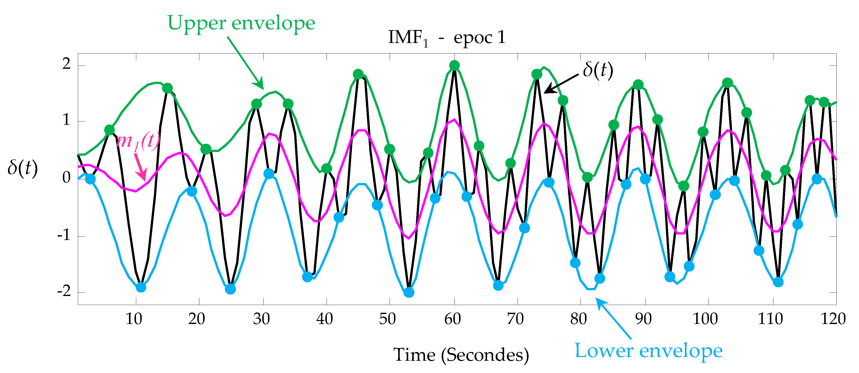
The EMD decomposes a signal denoted δ(t) into four steps:

• Step 1: The local extrema of δ(t) are identified and connected by a line to form an upper envelope (green line in Figure 3).
• Step 2: The local minima of δ(t) are identified and connected by a line to form a lower envelope (blue line in Figure 3).
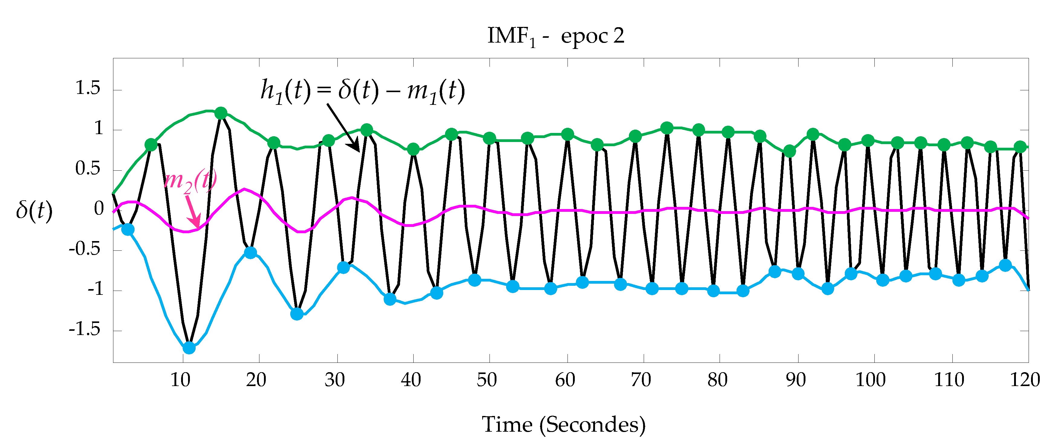
• Step 3: The average value of the upper and lower envelope is calculated and denoted m₁(t) (purple line in Figure 3). The subtraction of m₁(t) from δ(t) allows creating a component denoted h₁(t) as shown in Figure 4. The expression of h₁(t) is given as follows:

  $$\delta (t)-m_1(t)=h_1(t)$$

  (1)
• If h₁(t) satisfies the constraints of the IMF, then h₁(t) can be considered as the first IMF₁ of δ(t). If not, steps 1 to 3 will be applied to h₁(t) as shown in Equation (2):

  $$h_1(t)-m_{11}(t)=h_{11}(t)$$

  (2)

  where m₁₁(t) is the average value of the upper and lower envelope of h₁(t). This procedure is called the sifting process and is repeated k-times on h_1k(t) until the average line between the upper and lower envelopes is close to zero. This procedure is represented by the following equation:

  $$h_1{}_{(k-1)}(t)-m_1{}_k(t)=h_{1k}(t)$$

  (3)

The IMF₁, denoted c₁(t) with c₁(t) = h_1k(t), represents the high frequency component of δ(t). c₁(t) is then extracted from δ(t) in order to repeat the sifting process in a new component denoted r₁(t) (see Equation (4)):

$$\{\begin{array}{l}{r}_1(t)=\delta (t)-c_1(t)\\ r_n(t)=r_{n-1}(t)-c_n(t)\end{array}$$

(4)

A stop criterion must be defined to ensure that the signal obtained verifies the properties of an IMF, while limiting the number of iterations. The proposed criterion is based on the calculation of the relative variation of the signal between two consecutive iterations. It is given as follows:

$$CR={\displaystyle \sum _{t=0}^T\left[\frac{{\left|h_{1(k-1)}(t)-h_{1k}(t)\right|}^2}{h_{{}_{1(k-1)}}^2(t)}\right]}$$

(5)

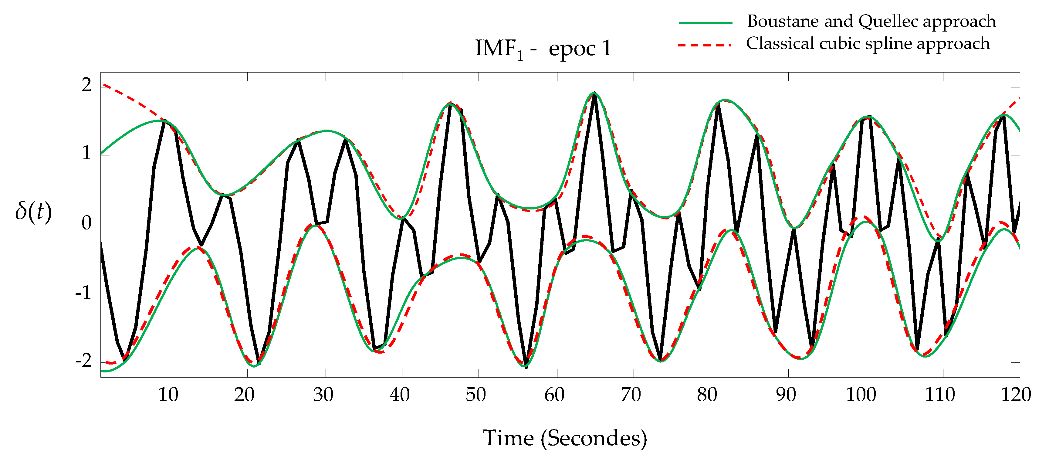
The upper and lower envelopes are obtained by an interpolation function. The interpolation function works on the minima (or maxima) values of the signal and on the corresponding abscissas. The problem here is that the first and last samples of the signal are not minima and maxima. So, there will be two intervals left with only one point to calculate the interpolation function, which is not possible. One solution would be to keep the computed interpolation polynomial over the adjacent interval. But as Figure 5 shows, the envelopes calculated with this solution (broken lines) are not satisfactory. To solve this problem, we added data at the start and end of the given interval, using the method proposed by Boustane and Quellec [34].

Let δ(t) be a time series of length T whose maximum and minimum envelopes must be determined and δ_max = {δ_max2,…, δ_{max T}} and δ_min = {δ_min2,…, δ_{min T}} is the set of maxima and minima.

-

We will fix the first point by applying the following rule:

♦

If: δ_min2 ≤ δ₁ ≤ δ_max2

• δ_max1 = δ_max2
• δ_min1 = δ_min2

♦

If not

• If δ increasing: δ_min1 = δ₁ and δ_max1 = δ_max2
• If δ decreasing: δ_max1 = δ₁ and δ_min1 = δ_min2

-

For the last point, we will apply:

♦

If: δ_{min T} ≤ δ_T ≤ δ_{max T}

• δ_{max T} = δ_{max T-1}
• δ_{min T} = δ_{min T-1}

♦

If not

• If δ increasing δ_{max T} = δ_T and δ_{min T} = δ_{min T-1}
• If δ decreasing δ_{min T} = δ_T and δ_{max T} = δ_{max T-1}

Figure 5 shows the interpolation of the extrema using a cubic spline. This figure shows that the method of Boustane and Quellec makes it possible to minimize the errors on the bounds of the interpolation interval (the envelopes in solid lines).

The implementation of the EMD method improved by the stop criterion and the avoidance of the edge effect is given by the following Algorithm 1:

Algorithm 1. Presentation of the different stages of the improved EMD

Step 1: Define a threshold μ: i ← 1 (i-th IMF) (μ = 0.25 in our case). Step 2: ri-1(t) ← δ(t) (residue). Step 3: Extract the i-th IMF. hi,k-1(t) ← ri-1(t); k ← 1 (k, iteration of the sifting process) Extraction of the maxima and minima points of hi,k-1(t) Calculation of the upper envelope $E_{i,k-1}^{up}(t)$ and lower envelope $E_{i,k-1}^{low}(t)$ by interpolation (Boustane and Quellec method) Calculation of the average envelope: $m_{i,k-1}(t)=\frac{E_{i,k-1}^{up}(t)+E_{i,k-1}^{low}(t)}{2}$ Update: hi,k(t) ← (hi,k-1(t)-mi,k-1(t)), k ← k + 1 Criterion stop calculation: $CR(k)={\displaystyle \sum _{t=0}^T\left[\frac{{\left|h_{i(k-1)}(t)-h_{ik}(t)\right|}^2}{h_{{}_{i(k-1)}}^2(t)}\right]}$ (T: length of the signal) Repeat steps (b) to (f) while CR(k) ≥ μ and affect IMFi (t) ← hi,k(t) (i-th IMF). Step 4: Update the residue ri(t) = ri-1(t)-IMFi (t) until the number of extrema in ri(t) is less than 2. Each extracted IMF is denoted ci(t) ← IMFi (t). Step 5: Repeat step 3 with i ← i + 1, until the number of extrema in ri(t) is less than 2.

The sifting process is repeated on r₁(t) n-times to obtain successive components with decreasing frequency bands. This procedure allows obtaining (n-1)-IMFs from the original signal δ(t). When r_n(t) becomes a monotonic function, the decomposition process can be stopped. The original signal δ(t) is composed by the (n-1)-IMFs in addition to the last component r_n(t) designated as a residue, as shown in the following equation:

$$\delta (t)={\displaystyle \sum _{i=1}^{n-1}{c}_i(t)+r_n}(t)$$

(6)

The IMFs c₁(t), c₂(t), …, c_n−1(t) include different frequency bands ordered from top to bottom. The frequency band contained in each component is different from another component. These frequency bands change according to the variation of the signal δ(t).

After the decomposition of δ(t) into IMFs, a Hilbert transform is applied to these latter in order to extract the instantaneous amplitude a_i(t) and frequency f_i(t). With the instantaneous amplitude a_i(t) and frequency f_i(t), it is possible to express the signal δ(t) by:

$$\delta (t)=PR{\displaystyle \sum _{i=1}^n{a}_i(t)\exp \left[j2\pi {\displaystyle \underset{0}{\overset{T}{\int }}{f}_i(t) dt}\right]}$$

(7)

where PR is real part and T is the length of the signal δ(t). This approach is analogous to the Fourier transform; it allows amplitude and frequency modulation simultaneously.

The instantaneous amplitude a_i(t) is obtained by the following equation:

$$a_i(t)=\sqrt{{\left(c_i(t)\right)}^2+{\left(H\left[c_i(t)\right]\right)}^2}1\le i\le n-1$$

(8)

With $H\left[c_i(t)\right]$: the Hilbert transform of c_i(t) expressed as follows:

$$H\left[c_i(t)\right]=\frac{1}{\pi }{\displaystyle \underset{-\infty }{\overset{+\infty }{\int }}\frac{c_i(\tau )}{t-\tau }} d\tau =c_i(t)\ast \frac{1}{\pi t}$$

(9)

where the symbol “*” denotes convolution operation.

We can define the instantaneous frequency f_i(t) as follows:

$$f_i(t)=\frac{1}{2\pi }\frac{d{\theta }_i(t)}{dt}$$

(10)

θ_i(t) is the instantaneous phase defined by the following equation:

$${\theta }_i(t)={\tan }^{-1}\left(\frac{H\left[c_i(t)\right]}{c_i(t)}\right)$$

(11)

For each IMF, the Hilbert spectrum density is defined as the square of the instantaneous amplitude:

$$H\left(f_i(t)\right)={\left(a_i(t)\right)}^2$$

(12)

H(f_i(t)) gives a local value of the energy in the time-frequency representation, and it is possible to extract the joint probability density p(f_i(t), a_i(t)) of the frequency and the amplitude from the set of the original series a_i and f_i for the IMFs set i = 1,…, n−1. This allows us to estimate the Hilbert marginal spectrum density:

$$h_i(f)={\displaystyle \underset{0}{\overset{\infty }{\int }}H\left(f_i(t)\right)dt}$$

(13)

The Hilbert marginal spectrum density is an energy density for a frequency f, which can be compared to the energy spectral density estimated by the Fourier transform. The objective of the proposed approach is to carry out the decomposition at the local level, in a time-frequency space.

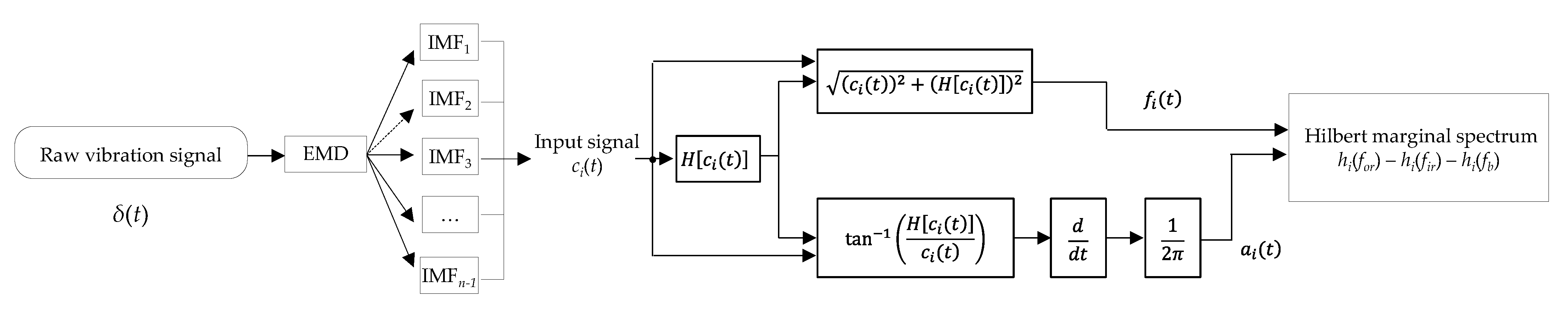
The implementation of the feature extraction approach is given by the following Algorithm 2:

Algorithm 2. Presentation of the health indicator algorithm

Apply the EMD to the vibration signal δ(t) Obtain the IMF $C_i(t){ }_{1\le i\le n-1}$. Apply the HT to each $C_i(t){ }_{1\le i\le n-1}$. Obtain instantaneous amplitudes of each $C_i(t){ }_{1\le i\le n-1}$. Obtain instantaneous frequencies of each $C_i(t){ }_{1\le i\le n-1}$. Calculate the Hilbert marginal spectrum density for each $C_i(t){ }_{1\le i\le n-1}$. Select the Hilbert marginal spectrum corresponding to the frequency bands of bearings failures.

The flowchart given in Figure 6 summarizes the steps of an automatic extraction of the Hilbert spectrum density related to the three characteristic frequencies f_or, f_ir, and f_b corresponding, respectively, to the frequencies of the outer race, inner race, and balls:

3. Comparison of the Proposed Approach with Wavelet Analysis

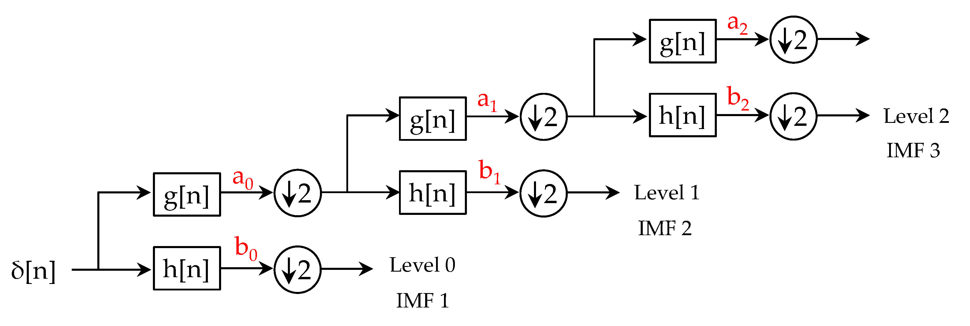
The EMD decomposition of a signal δ(t) shows that the components are classified locally from the highest frequencies to the lowest frequencies. The first modes have the fastest oscillations and the last modes have the slowest oscillations. The EMD can be considered as a self-adapting and automatic filter. The EMD can therefore be used as a signal denoising tool. It is therefore natural to compare it with the wavelet analysis. The wavelet decomposition is an iterative process that decomposes the signal δ(t) using a high-pass filter and a low-pass filter in quadrature. The high-pass filter is achieved by the convolution of the signal and the chosen wavelet. With a mean value equal to zero, the chosen wavelet captures the rapid variations of the signal h(t). On the other hand, the second signal g(t), coming from the low-pass filter, is downsampled, and the process is applied recursively, as shown in Figure 7. From a theoretical point of view, this downsampling consists of dividing by 2 the frequency of the wavelet and therefore capturing lower frequencies. In this sense, the EMD and discrete wavelet transform algorithms both analyze the signal starting with the extraction of details and ending with the low-frequency components. However, and unlike wavelets, the EMD is a non-parametric approach that does not require a projection basis. This is a non-linear temporal decomposition not involving an external function (mother wavelet) with a predetermined basis, while the results with the wavelet transform depend on the choice of the wavelet. Moreover, the EMD is a local, iterative, adaptive approach that describes the signal as local oscillatory components going from the high to low frequencies while the wavelet method is a parametric approach that describes the signal in two categories, the details and approximations, by ordering them from lower to higher frequencies.

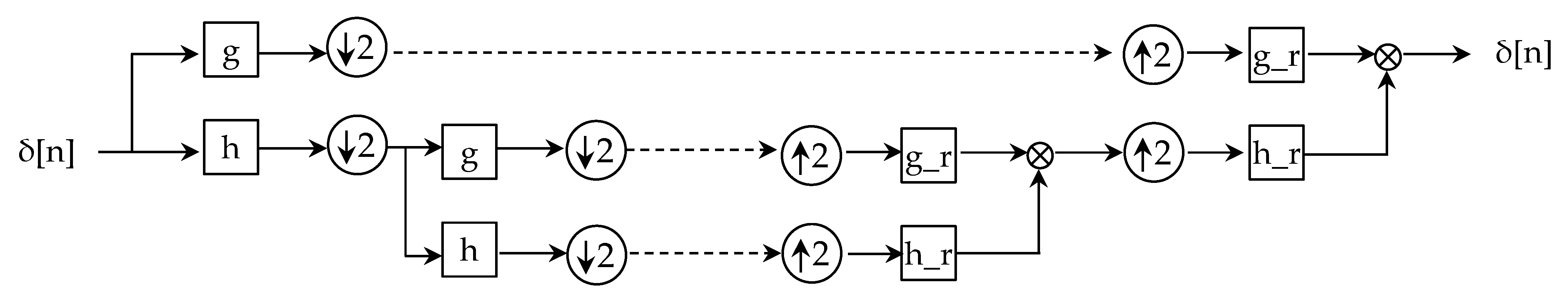
One of the advantages of the EMD method is the simplicity and the rapidity of denoising a signal by reconstituting the original signal as demonstrated by formula (6). This principle is noted reciprocity. This reciprocal is a transformation often analogous to the decomposition as it is the case in the reconstruction of the wavelet where the components must be treated by the mirror filters in the reverse order of the decomposition, as illustrated in Figure 8. On the other hand, the EMD carries out extractions of signals by successive subtraction of IMF, which makes the reconstruction fast and visual because it consists of a simple summation. In this sense, the EMD has an asymmetric character atypical of signal decompositions.

Another advantage of the EMD is the stop criterion and its adaptability. Indeed, in the wavelet transform, a sub-sampling is carried out. The algorithm terminates due to finite precision of the data, but the decomposition is theoretically infinite. This stop criterion has practical interest since one can know in advance the number of components that it will be necessary to calculate. In contrast, the EMD is based on the variations of the signal for extraction of the IMFs. The number of IMFs cannot be predicted in advance. This is both a drawback and strength of the algorithm because one might think that there is a better correspondence between an IMF and the origins of its oscillations. As noted previously, the EMD therefore adapts better to the input data, and this without the choice of parameters for the decomposition (type of wavelet, number of sub-samples to be performed, etc.).

4. Experimental Results

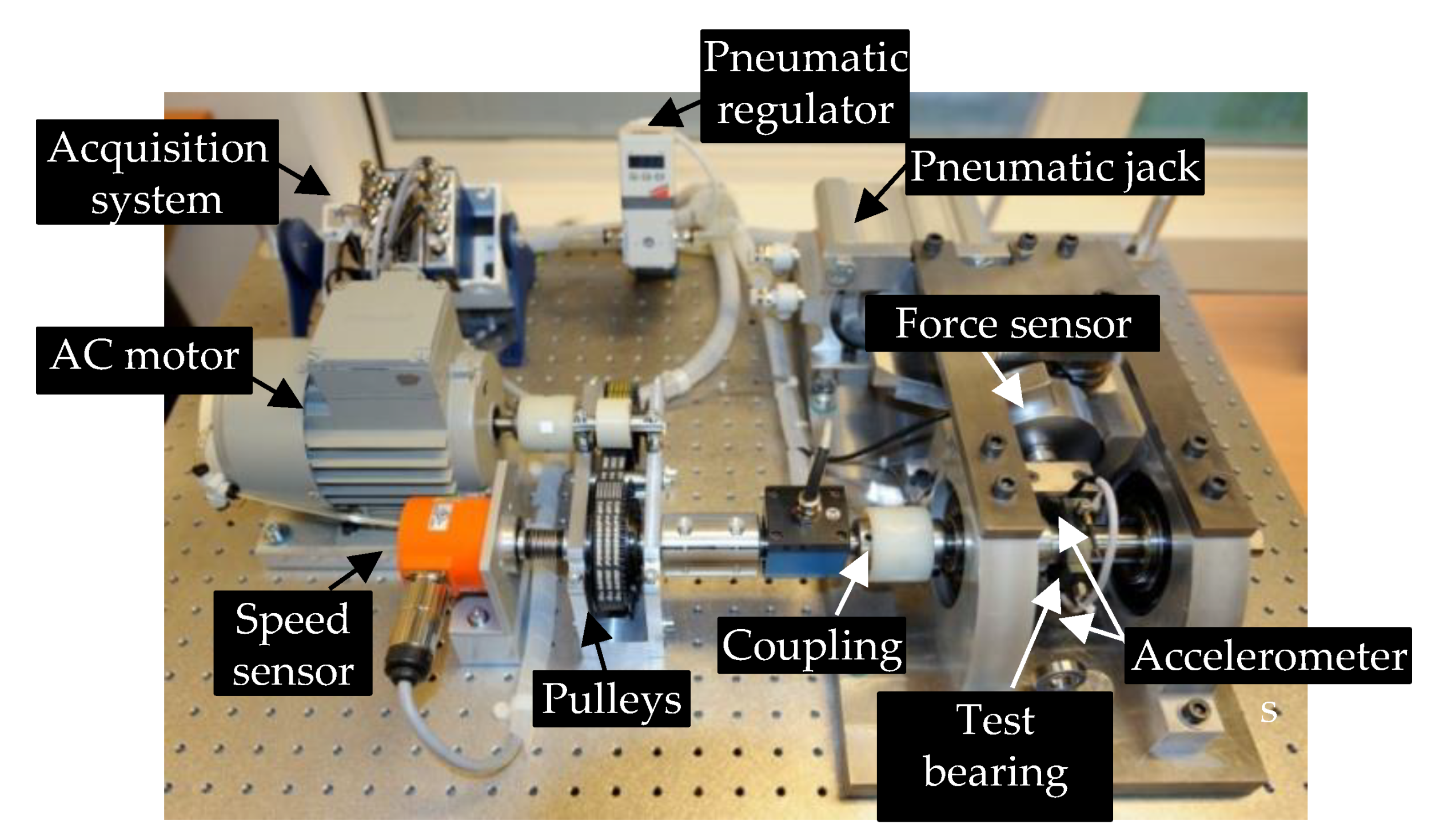
First, tests were conducted on NSK 6804RS ball bearings to show the efficiency of the feature extraction approach and to show also the limits of the statistical method for monitoring ball bearings (Bbs). The characteristics of the studied Bbs are given in

Table 1. NSK 6804RS ball bearing characteristics.

Ball diameter (mm)	3.5
Number of rollers	13
Diameter of outer race (mm)	29.1
Diameter of inner race (mm)	22.1
Bearing mean diameter (mm)	25.6

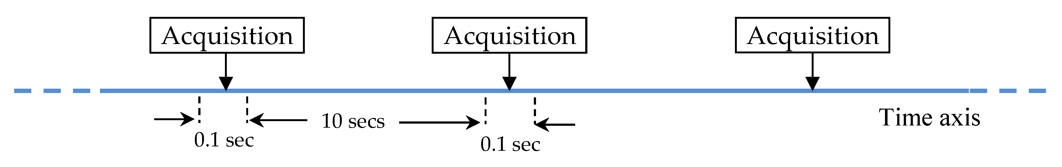
. Tests on Bbs corresponded to accelerated aging tests obtained by the application of a radial overload of 4000 Newtons. The used aging test bench was called “PRONOSTIA” [35] (see Figure 9). The chronogram of the aging tests is represented in Figure 8. In these tests, Bbs were subjected to constant stresses in speed and load. As shown in Figure 10, the chronogram is composed of a time axis showing the periodicities of vibration signal records (see arrows). The acquisition steps were measurement steps intended to record and verify the state of Bb degradation. Vibration signals were recorded every 10 s with a sampling frequency of 25.6 kHz.

Probability calculations allowed the estimation of bearing life for a given application, but these estimations only took into account the phenomenon of fatigue (a natural phenomenon of aging in a bearing). The nominal life corresponded to the number of revolutions that at least 90% of bearings can perform under the same conditions before the appearance of the first signs of fatigue. It is denoted L₁₀:

$$L_{10}={\left(\frac{C}{P}\right)}^{\beta }$$

(14)

with:

• P: equivalent radial load applied on the bearing in Newtons (N).
• C: dynamic load supported by a bearing to achieve a nominal life of 1 million revolutions, in N.
• β is a coefficient where: $\{\begin{array}{c}\beta =3 \mathrm{for} \mathrm{ball} \mathrm{bearings}\\ \beta =\raisebox{1ex}{$10$}\!\left/ \!\raisebox{-1ex}{$3$}\right.\mathrm{for} \mathrm{roller} \mathrm{bearings}\end{array}$.

If the speed of the Bb is constant, we can express the bearing life in hours by:

$$L_{10h}=\frac{{10}^6}{60n}{\left(\frac{C}{P}\right)}^{\beta }$$

(15)

with:

• n: rotation speed in rpm.

Formula (15) gives a life estimation of the NSK 6804RS ball bearing for the degradation conditions (CD₁ and CD₂) described as follows:

-

CD₁: rotation speed of 1800 rpm and a radial load of 4000 N → L10 h = 9 h 15 min

-

CD₂: rotation speed of 1650 rpm and a radial load of 4200 N → L10 h = 8 h 43 min

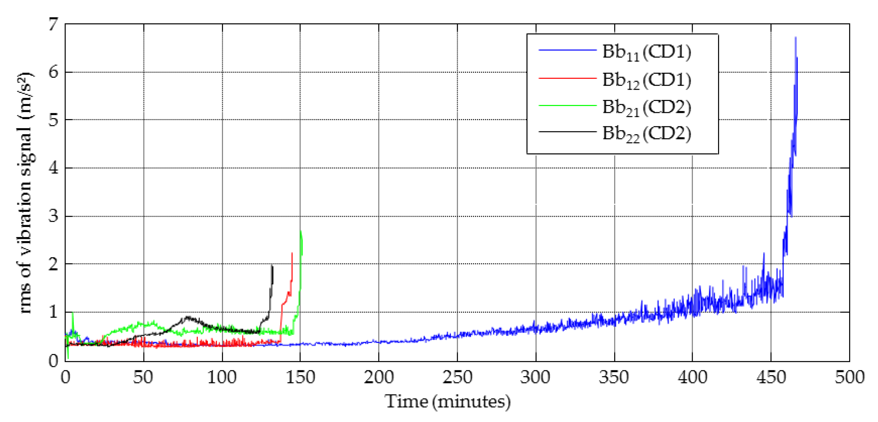
Two ball bearings were tested for each degradation condition (CD). For CD₁; the bearings were respectively numbered Bb11 and Bb12. The first number corresponded to the CD, and the second number corresponded to the number of the tested bearing. For CD₂, bearings were respectively numbered Bb21 and Bb22. As shown in Figure 11, the Bbs (11 and 12), in CD₁, were degraded after 7 h 25 min and 2 h 25min, respectively.

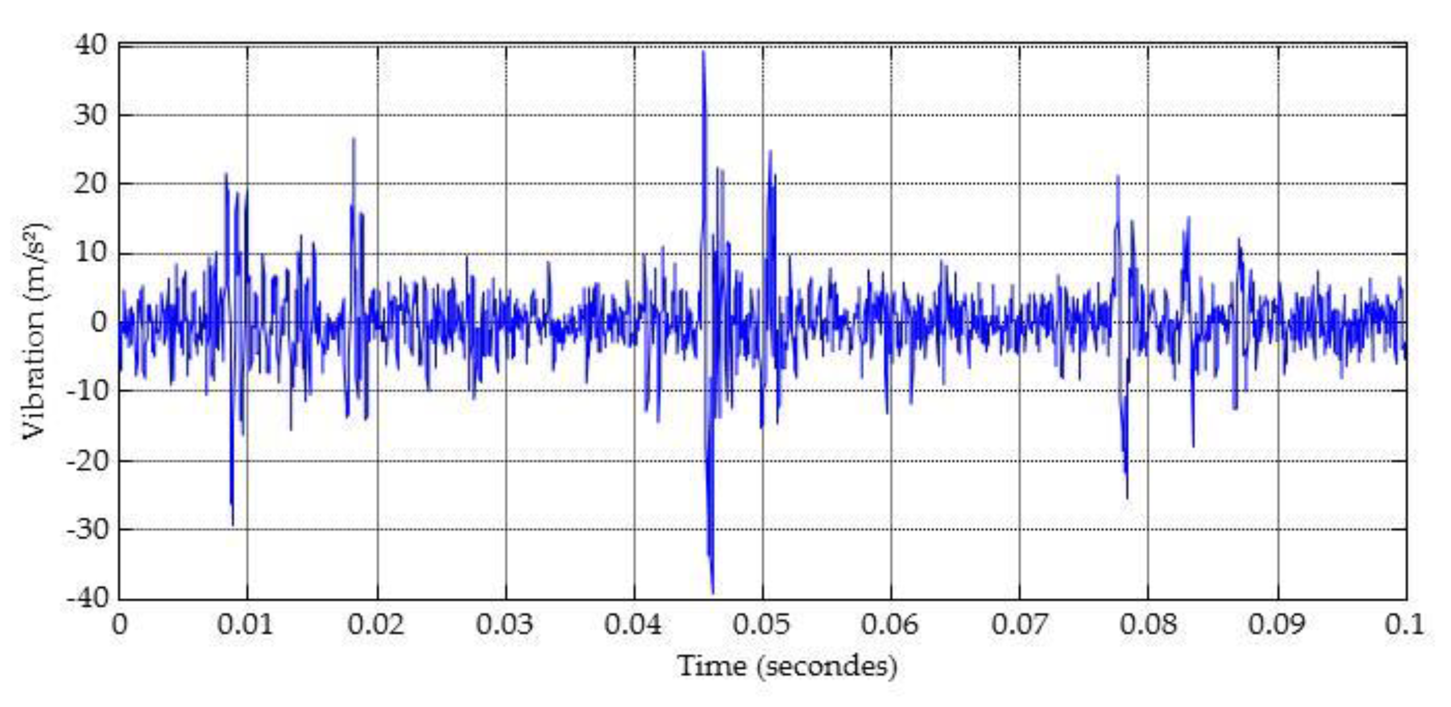
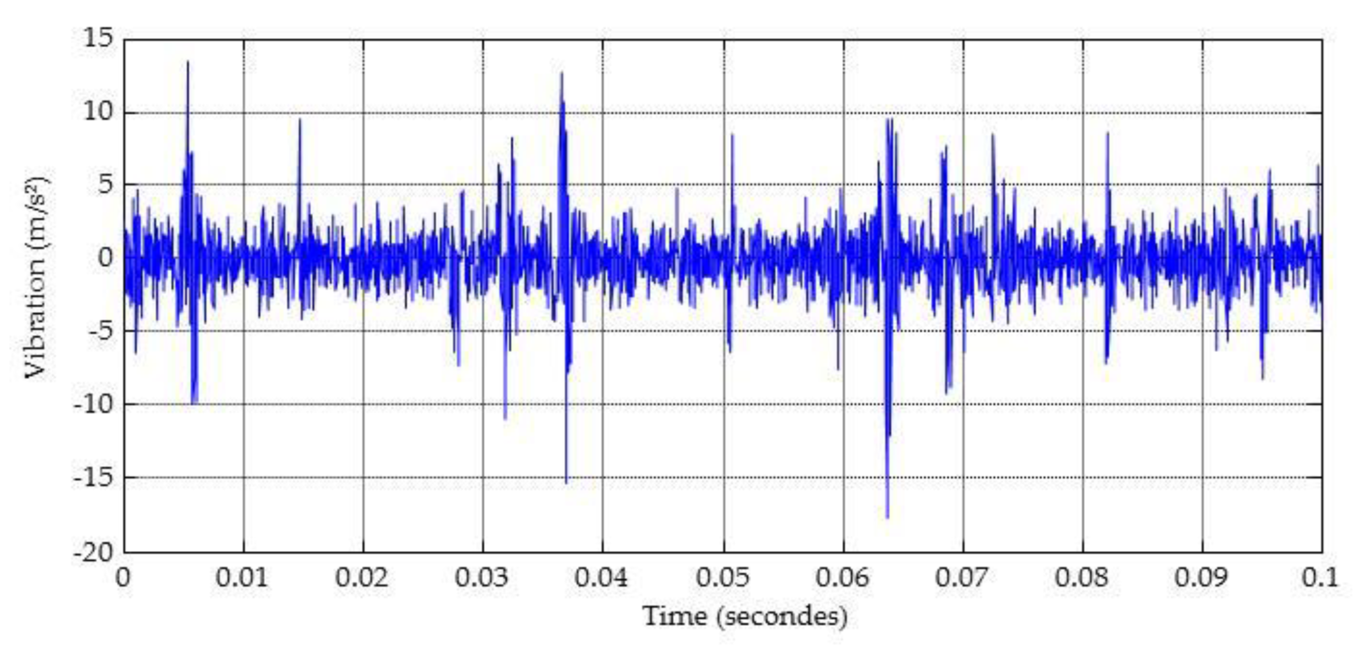
These results indicated a mismatch between the expected life given by the manufacturer (see formula (15)) and those observed for the tested bearings 11 and 12. These results also revealed a large gap between bearings 11 and 12, of 5 h 50 min. Figure 12 and Figure 13 show the vibration signals of bearings 11 and 12, respectively. These signals corresponded to defective bearings when the acceleration exceeded 20 m/s².

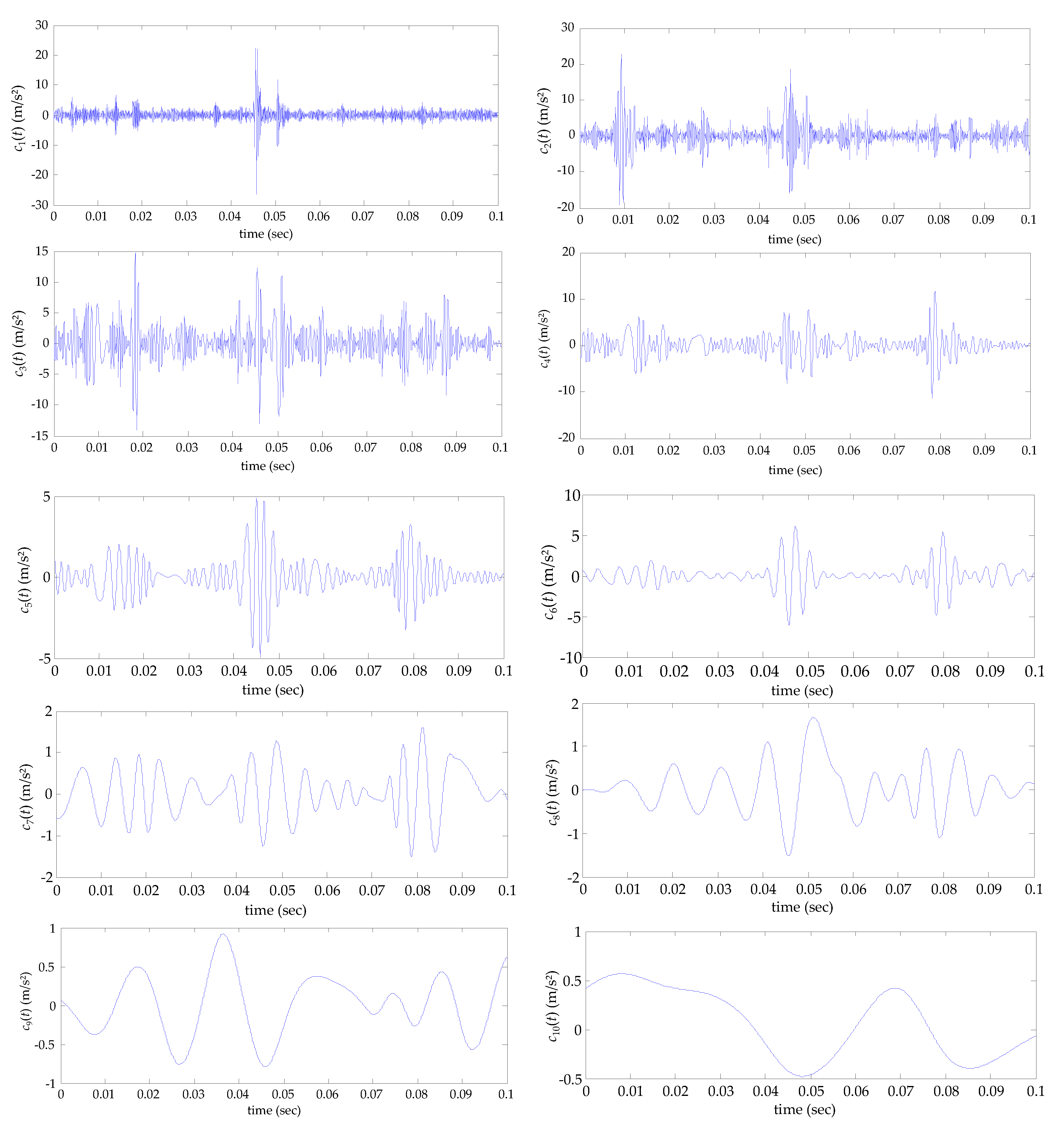
We can notice from these two figures that the acceleration peaks exceeded 20 m/s² for bearing 11 and 13 m/s² for bearing 12. If we consider bearing 11 as a defective bearing, this corresponded to an rms (Root Mean Square) equal to 6.7 m/s² (see Figure 11). The rms of bearing 12 was equal to 2.1 m/s². Even if an rms of 2.1 m/s² was a high value compared to a healthy bearing, which equals 0.45 m/s², does it mean that bearing 12 was defective. In addition, there was no visible periodicity between the acceleration peaks giving an indication of its fault frequency. The empirical mode decomposition (see Figure A1 in Appendix A) followed by a Hilbert transform on the vibration signal of the Bb11 makes it possible to obtain the Hilbert spectrum of each IMF (see Figure 14).

Our approach was based on filtering the vibration signals around the characteristic frequencies of bearing faults. Formulas for calculating the characteristic fault frequencies of bearings are given as follows:

$$f_{or}=\frac{n_b}{2}\cdot f_r\cdot \left[1-\frac{BD}{PD}\cdot \cos \psi \right]$$

(16)

$$f_{ir}=\frac{n_b}{2}\cdot f_r\cdot \left[1+\frac{BD}{PD}\cdot \cos \psi \right]$$

(17)

$$f_b=\frac{PD}{BD}\cdot f_r\cdot \left[1-\frac{B{D}^2}{P{D}^2}\cdot {\cos }^2\psi \right]$$

(18)

with:

-

f_ir: characteristic frequency of the inner ring;

-

f_or: characteristic frequency of the outer ring;

-

f_b: characteristic frequency of the ball;

-

f_r: frequency of rotation of the rotor;

-

Ψ: contact angle;

-

n_b: number of balls;

-

BD: ball diameter;

-

PD: pitch diameter of the bearing.

For a rotation speed of 1800 rpm (f_r = 30 Hz), and for the geometry of the NSK 6804RS ball bearing, we obtain:

-

f_or = 168 Hz;

-

f_ir = 221 Hz;

-

f_b = 215 Hz.

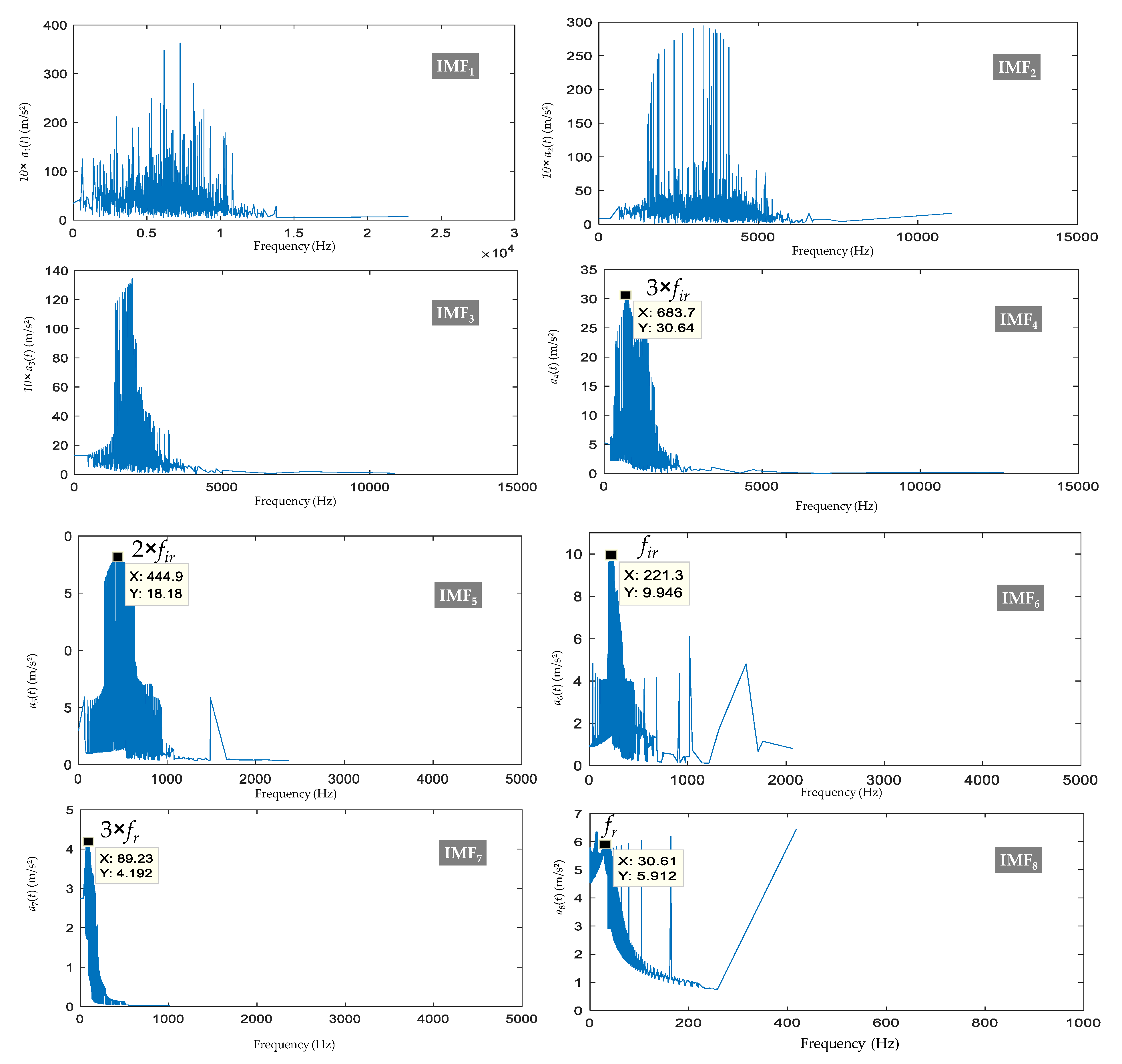
The Hilbert spectra of IMFs 4–8 allow us to identify the frequency corresponding to the rotation speed (30 Hz) and the frequency corresponding to the inner race fault (f_ir). However, IMFs 1–3 do not show significant anomalies (the amplitude of the defect is embedded in the noise). These spectral anomalies may be due to the following:

-

Transmission belt in poor condition: The poor condition of a “V” belt (variation in width, deformation) creates variations in tension able to induce vibrations of frequency equal to the rotation of the belt. If the pulleys are not properly aligned, there will be an axial component inherent in this vibration.

-

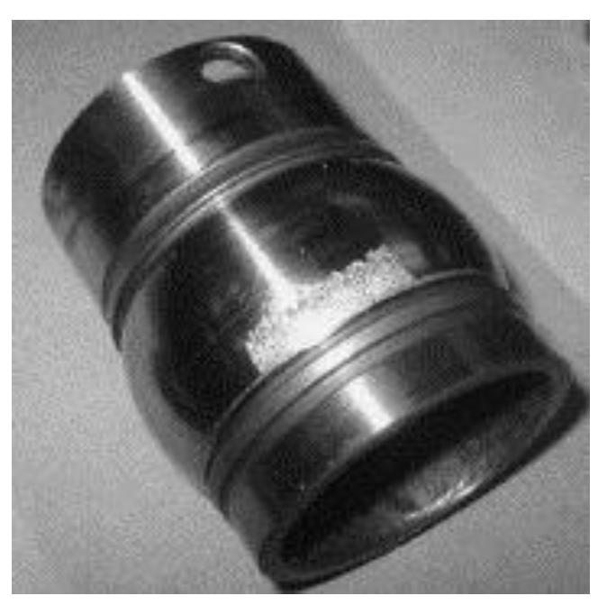
Chipping of bearings: Chipping of a bearing railway causes shocks and bearing resonances that are easily identified with a shock-wave measuring device. In spectral analysis, this phenomenon appears at high frequencies with a spectral density that increases when the bearing deteriorates. If the bearing damage only included a single point, a peak could appear at a frequency linked to the speed of the bearing and to the dimensions of the bearing (diameter of inner and outer race, number of balls).

-

Friction: The friction of surfaces with asperities generates vibrations generally located in the high-frequency range. The state of the surface and the nature of the materials in contact have an influence on the intensity and frequency of the vibrations thus created. These phenomena are often sporadic and therefore difficult to analyze and monitor.

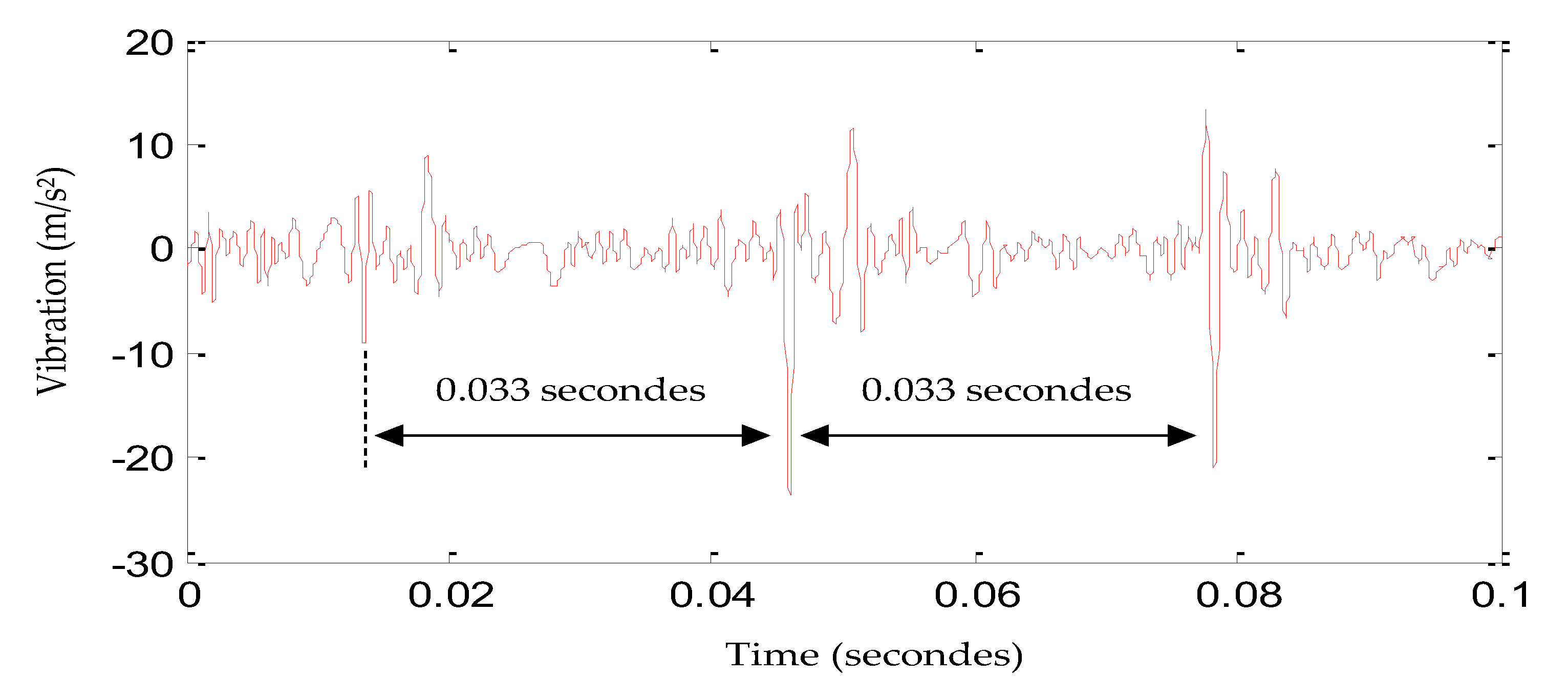
Given that the vibration signal δ(t) of Bb11 is the sum of the IMFs, the filtration of the high frequencies is obtained by summing the IMFs, which allows the low frequencies to appear. We thus obtain Figure 15. This figure shows a filtered vibration signal. We can observe a periodicity of 0.033 s corresponding to the rotation speed of 1800 rpm (30 Hz). The rms of this signal is equal to 3 m/s². We can also observe from Figure 16, Figure 17 and Figure 18 that the spectrum of the 6th-IMF indicates strong amplitudes around the characteristic frequencies of the defects of Bb NSK 6804RS.

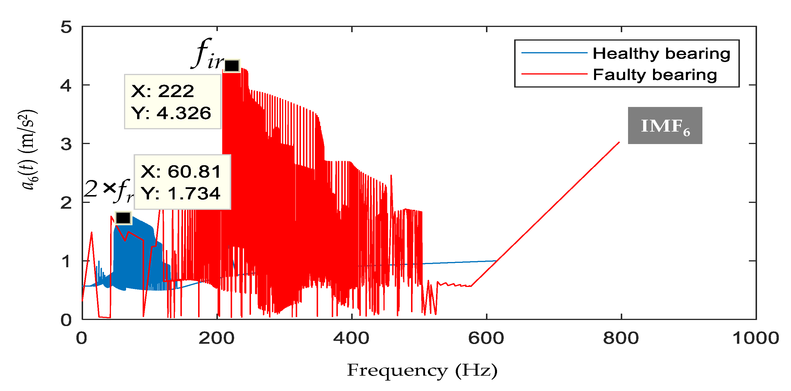
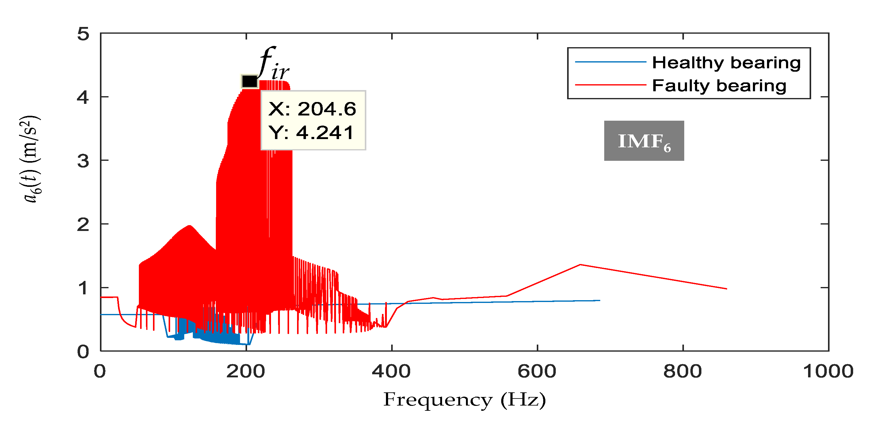
By repeating the same steps on the vibration signal of bearing 12, we obtain Figure 19:

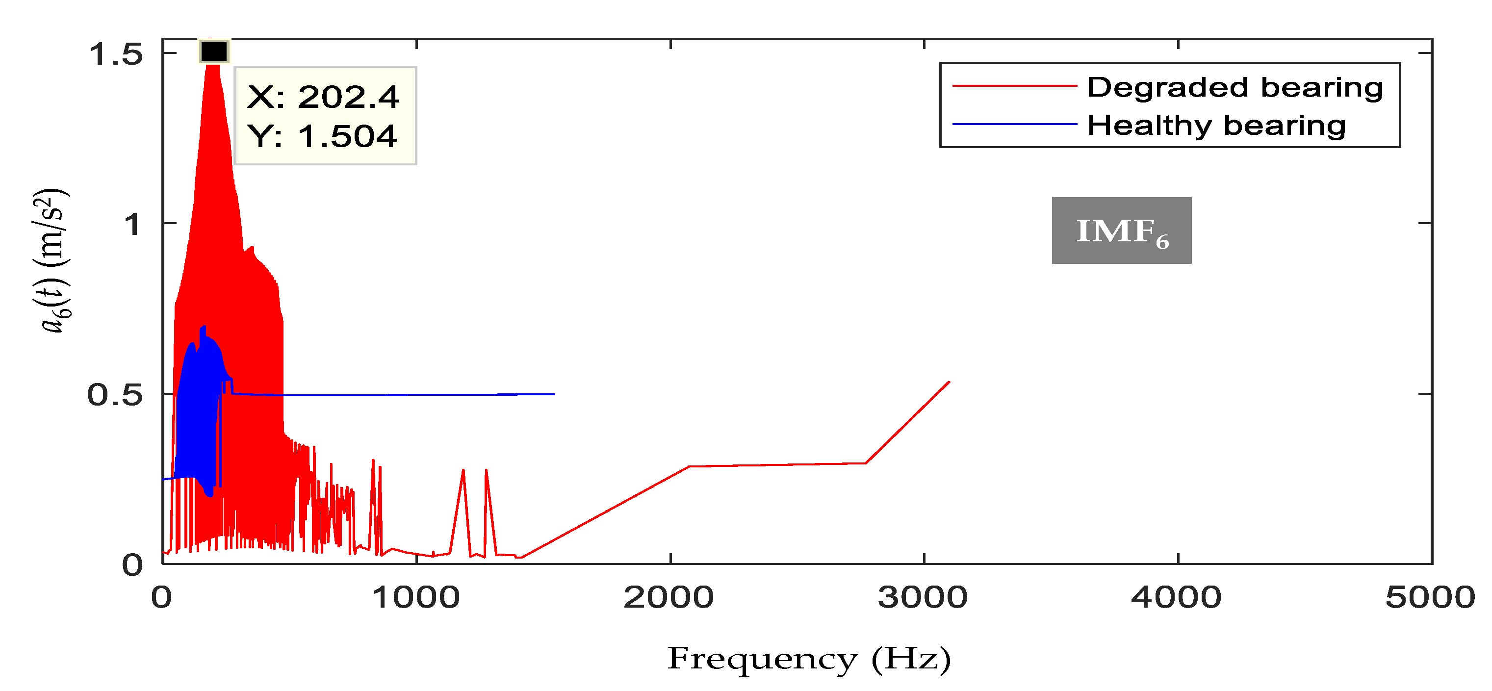
In the Bb12, the Hilbert spectrum of IMF 6 was equal to 4.3 m/s² around 222 Hz and therefore around the characteristic frequencies of the inner race (see Figure 17). The same point may be made for the Bb11, where the amplitudes in the IMF6 spectrum were equal to 9.9 m/s² (see Figure 16). For Bb 21, we can see from Figure 16 that the maximum amplitudes in the IMF6 spectrum were around 204 Hz. Using the Formulas (16)–(18) for a rotation speed of 1650 rpm (f_r = 27.5 Hz) and the geometry of the NSK 6804RS ball bearing, we obtain: f_r = 154 Hz, f_ir = 203 Hz, f_b = 197 Hz. It is clear from Figure 18 that the increase of the amplitude around 204 Hz was due to an inner race and ball defect.

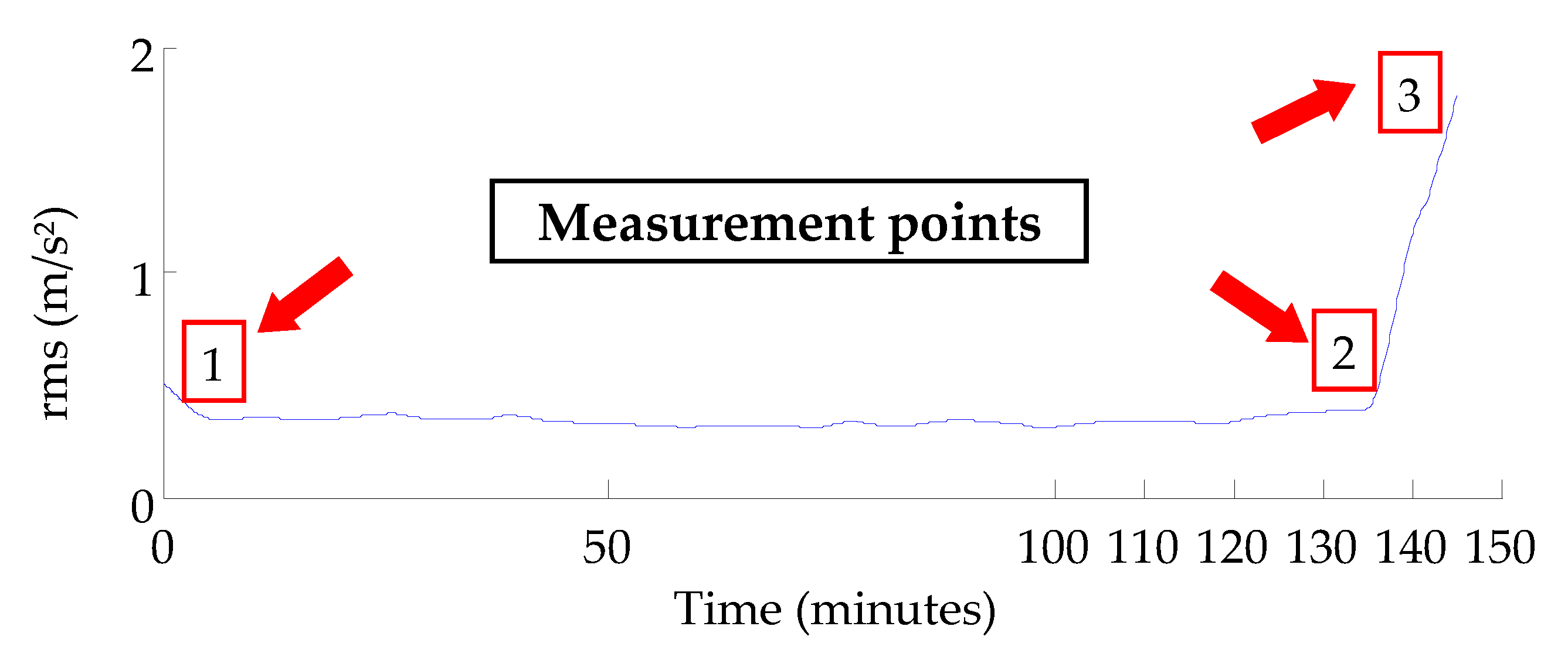
Each Bb operated under very specific constraints. We can see from Figure 16, Figure 17 and Figure 18 that Hilbert spectrum amplitudes located around the fault frequencies of Bbs 11, 12, and 21 were clearly distinct and quantifiable in term of severity. We can conclude that this method allows detecting, locating, and quantifying the severity of degradation for a given speed and load. 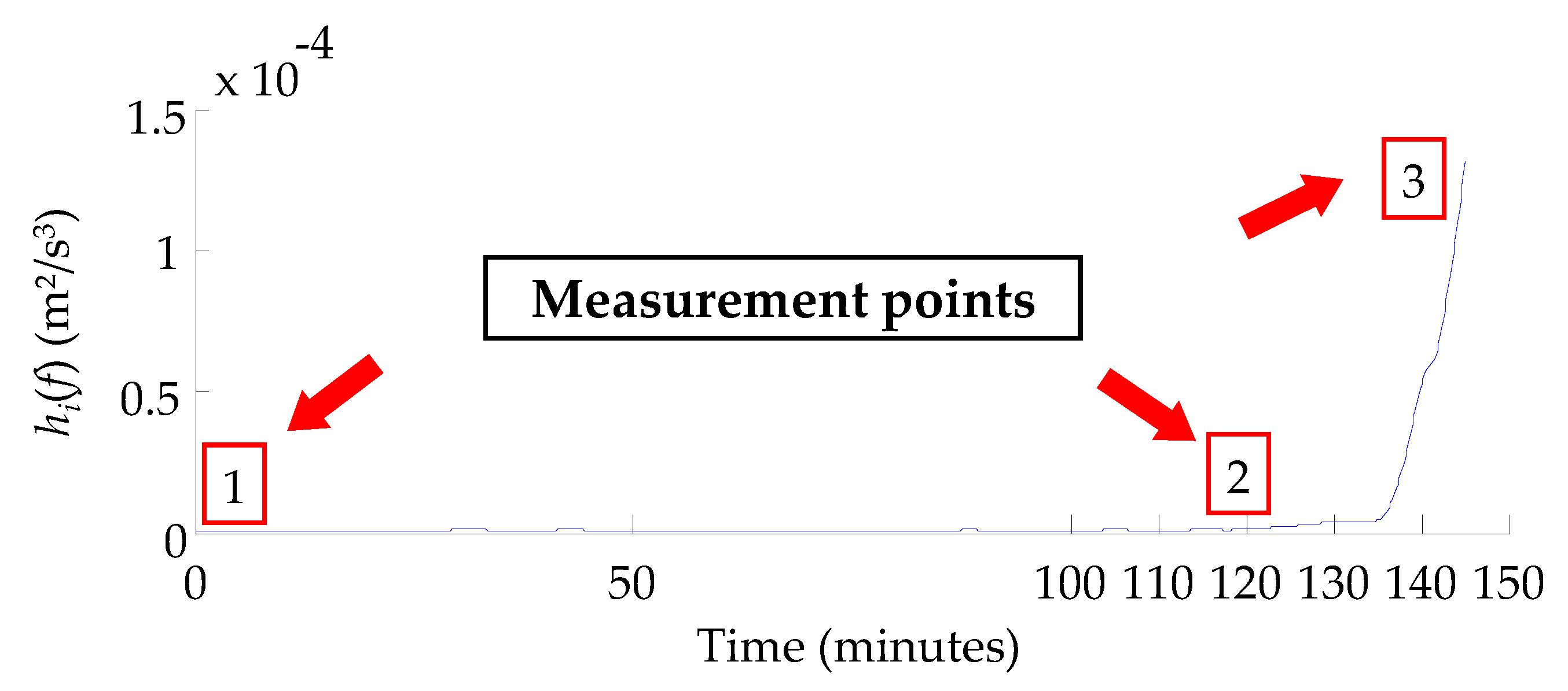In fact, if we take the case of Bb21, we can see from Figure 20 and Figure 21 that the degradation of Bb12 was reflected by the Hilbert marginal spectrum and the rms. In Figure 21, the classical rms of the vibration signal of Bb12 is represented. We chose three measurement points. The first point corresponded to the beginning of the test. This measurement corresponded to a Bb in good health. The third measurement was taken at the end of the test and represented a faulty Bb. The second measurement point was taken when the first signs of degradation were detected. By comparing the two figures, it can be said that it is easier to follow the evolution of the degradation of a bearing by filtering and extracting its Hilbert marginal spectral density in order to detect the first signs of degradation. The first signs of degradation were detected at t = 122 min for our indicator while for the rms, the detection was validated only after 140 min into the test. It was explained in [36] that classical spectral analysis cannot detect rolling defects due to the presence of background noise and the randomness of the vibrations. By applying the proposed approach, it is possible to follow the degradation of the Bb at the beginning, as shown in Figure 22. Figure 20 shows the Hilbert spectrum of the vibration signal recorded after 122 min into the test (point 2 in Figure 20). With this figure, we can see that the beginning of the degradation was due to an anomaly in the inner race of the bearing.

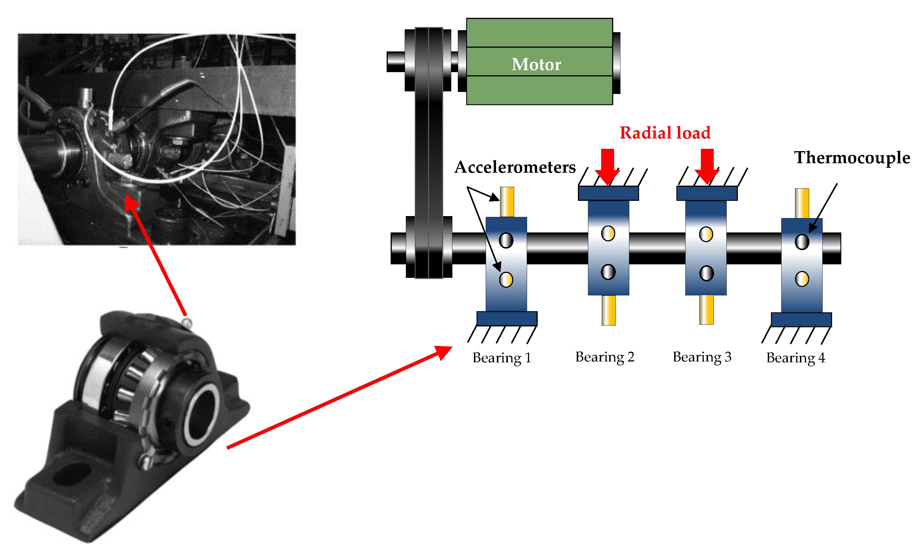
In order to verify the validity of this method for other types of bearings, we decided to use it to detect the appearance of defects in roller bearings. A database corresponding to the accelerated aging of four roller bearings was used. These bearings were placed on a test bench designed by Rexnord Corp. The test bench was composed of four ZA-2115 roller bearings placed on a shaft, as shown in Figure 23. The characteristics of these bearings are detailed in

Table 2. Roller bearing characteristics.

Roller diameter (mm)	8.4
Number of rollers	16
Pitch diameter (mm)	71.62
Contact angle (°)	15.17

.

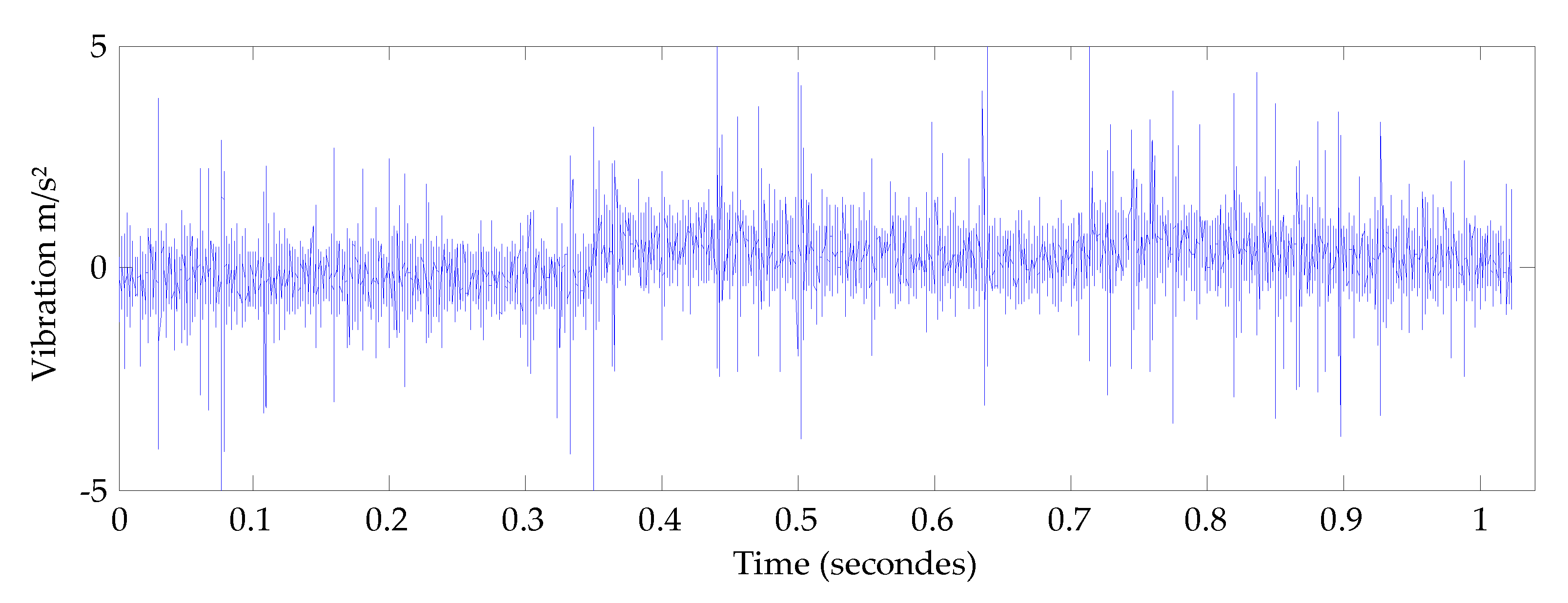
The rotation speed was fixed at 2000 rpm and a radial load of 26,689 N was placed on the shaft and bearings by a spring mechanism. Vibration signals were recorded every 10 min with a sampling frequency of 20 kHz. The vibration signal of bearing number 3, recorded on the last day of testing, was used to assess the performance of the proposed approach. This signal corresponded to an inner race fault. The vibration signal of bearing 3 is shown in Figure 24:

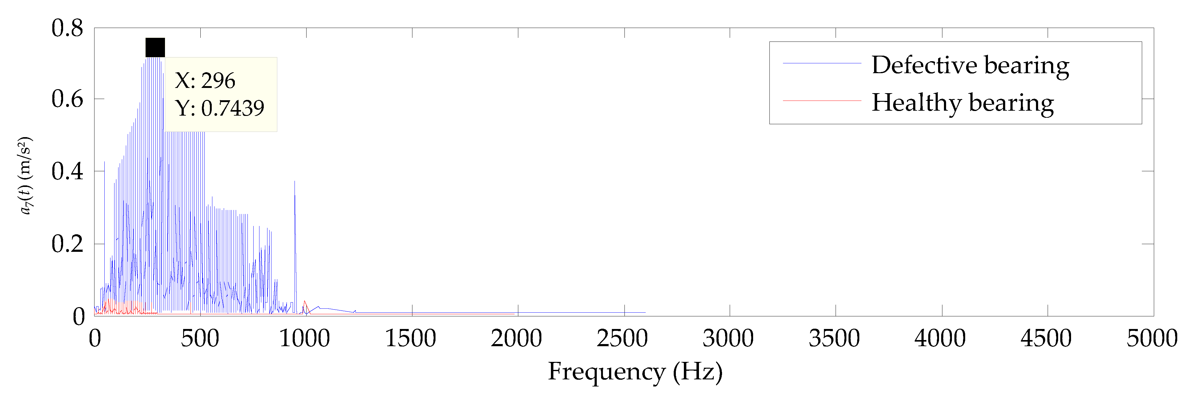
From this signal, the EMD and the HT were performed in order to obtain the marginal spectral density of each IMF. Fifteen IMFs we obtained. Knowing the rotational speed of the bearings and their characteristics, we were able to deduce the frequency of faults. They are given as follows:

-

Outer ring fault: 236.4 Hz;

-

Inner ring fault: 296.8 Hz;

-

Roller fault: 280.8 Hz.

The Hilbert spectrum amplitudes of IMFs 1 to 6 indicated that the low-frequency spectrum showed no significant anomalies. On the other hand, IMF 7 indicated high peaks (0.74 m/s²) around 296 Hz and therefore around the characteristic frequencies of the inner ring (see Figure 25 and Figure 26).

5. Conclusions

This paper presented an approach for the condition monitoring of bearings based on the EMD and the HT. As presented previously, the EMD decomposed the studied signal into IMFs. These components were classified locally from the highest frequencies to the lowest frequencies. This reflected a behavior in a bank of self-adaptive and automatic filters of the EMD and its interest in signal denoising. However, some errors related to the principle of EMD affect the quality of signal decomposition. Indeed, EMD decomposition has certain limitations linked to its basic principle, which makes use of the sifting process, interpolation, to determine the upper and lower envelopes, or to the nature of the studied signal, its sampling. The most important errors are due to the boundary effects and accumulations of errors introduced by the sifting algorithm and interpolation (Gibbs phenomenon). A solution was proposed to solve the problem of the boundary effects. The obtained results demonstrated the effectiveness of the proposed approach for the detection and diagnosis of bearing defects (ball or roller) for different speeds and loads. Implementing the EMD requires making choices, especially with regard to the criteria for stopping the sifting process, which is deeply linked to the free interpretation of the zero local mean value in the definition of an IMF. Another negative point is the fact that the EMD is very sensitive to boundary errors. The final drawback of the presented EMD was its lack of analytical expression. Because the EMD is an algorithm, there is no underlying mathematical foundation for this decomposition, such as Fourier or wavelets transforms.

6. Perspectives

In addition to detecting the presence of a defect and locating it, it would also be interesting to identify the different degradation stages before they appear. We therefore recommend retesting the NSK 6804RS ball bearings under less severe operating conditions than those presented previously. Based on formula (15), the life of the NSK 6804RS ball bearing for the new degradation conditions (CD₁, CD₂ and CD₃) is given as follows:

-

CD₁: rotation speed of 1800 rpm and a radial load of 2000 N → L10 h = 74 h 04 min

-

CD₂: rotation speed of 1650 rpm and a radial load of 2500 N → L10 h = 41 h 22 min

-

CD₃: rotation speed of 1500 rpm and a radial load of 3000 N → L10 h = 26 h 20 min

In addition to the steady state, two other types of aging tests need to be considered:

• Non-stationary tests (NS1): ball bearings are subjected to constant stresses in speed and variable stresses under load;
• Non-stationary tests (NS2): ball bearings are subjected to constant stresses under load and variable stresses in speed.

Tests in non-stationary state (NS1):

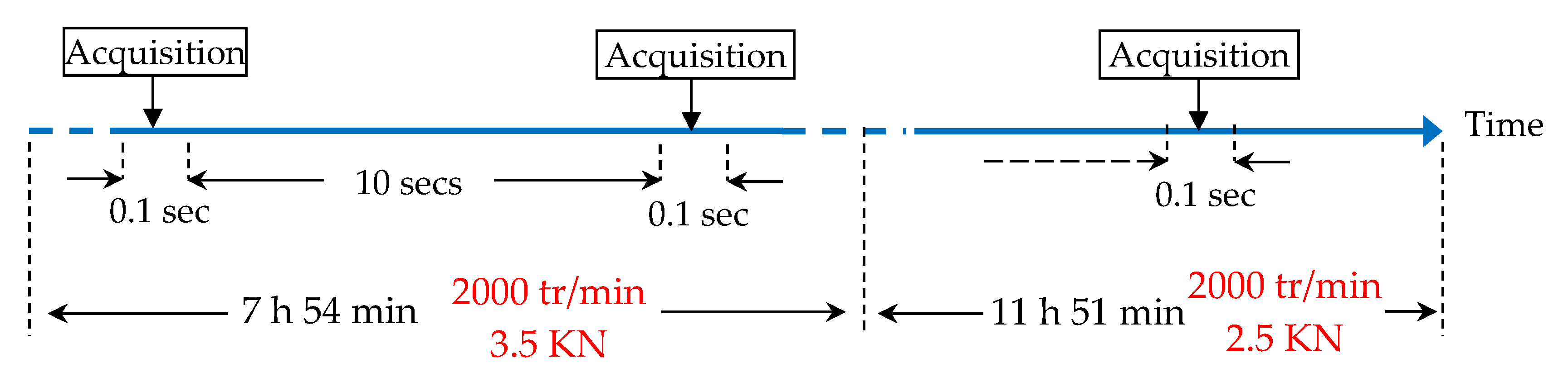
The proposed timing diagram used for aging in the non-stationary state (NS1) is presented in Figure 27. The Bbs will be subjected to a constant speed of 2000 rpm and a radial load varying between 2.5 and 3.5 kN. When a Bb is subjected to a variable load and a constant speed, an equivalent load can be used to determine the life of the Bb. It is given by the following formula:

$$C_{eq}={\left(t_1·C_1^{\alpha }+t_2·C_2^{\alpha }+\dots +t_z·C_z^{\alpha }\right)}^{{\alpha }^{-1}}$$

(19)

-

C_eq: Equivalent load applied to the bearing during the test;

-

t_i: Duration of load use with: ${\displaystyle \sum _{i=1}^z{t}_i=1}$;

-

C_i: Applied load in the Bb for a period t_i;

-

α: Constant equal to 3 for a ball bearing and 10/3 for a roller bearing.

If a load of 3.5 kN is applied to the Bb for 40% of the test duration and then 2.5 kN in the remaining duration (60%), then the equivalent load will be 3 kN. The lifetime of the Bb will be equal to 19 h 45 min. In the end, we would apply a radial load of 3.5 kN for 7 h 54 min, then a radial load of 2.5 kN for 11 h 51 min.

Tests in non-stationary state (NS2):

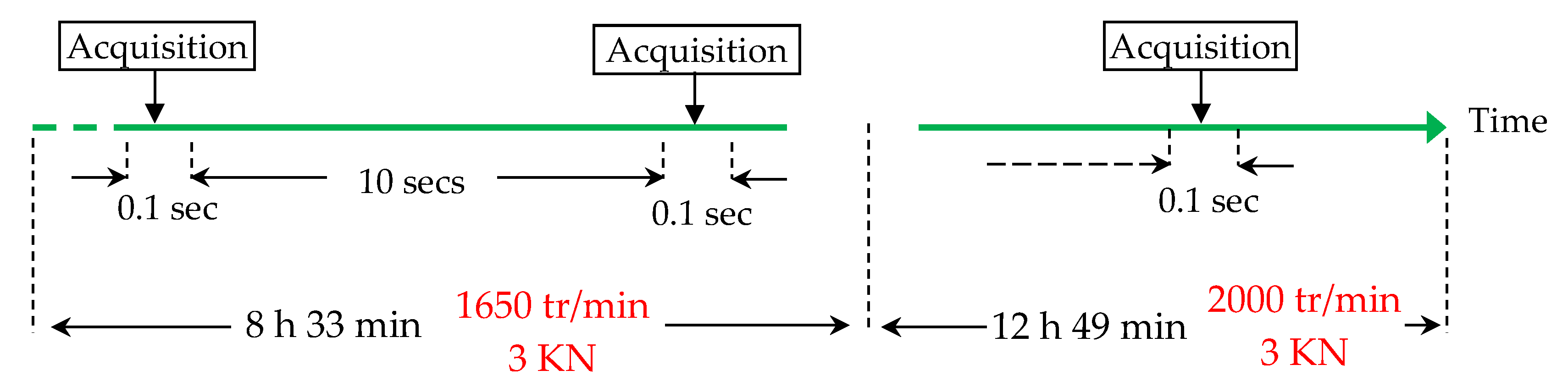
The chronogram used for aging in the non-stationary test (NS2) is presented in Figure 28. The Bbs will be subjected to a constant radial load of 3 kN and a speed which varies between 1650 and 2000 rpm. When a Bb is subjected to a variable speed and a constant load, an equivalent speed can be used to determine the life of the Bb. It is given by the following formula:

$$V_{eq}=t_1·V_1^{}+t_2·V_2^{}+\dots +t_z·V_z^{}$$

(20)

with:

-

V_eq: equivalent speed applied to the Bb during the test;

-

V_i: rotation speed applied to the Bb for duration t_i.

If a rotation speed of 1650 rpm is applied to the Bb for 40% of the test duration and then 2000 rpm for the remaining duration (60%), then the equivalent speed will be equal to 1860 rpm. The lifetime of the Bb will be equal to 21 h 23 min. In the end, we would apply a speed of 1650 rpm for 8 h 33 min, then a speed of 2000 rpm for 12 h 49 min.