
Development of AI-Based Diagnostic Model for the Prediction of Hydrate in Gas Pipeline


Abstract
1. Introduction
2. Methods
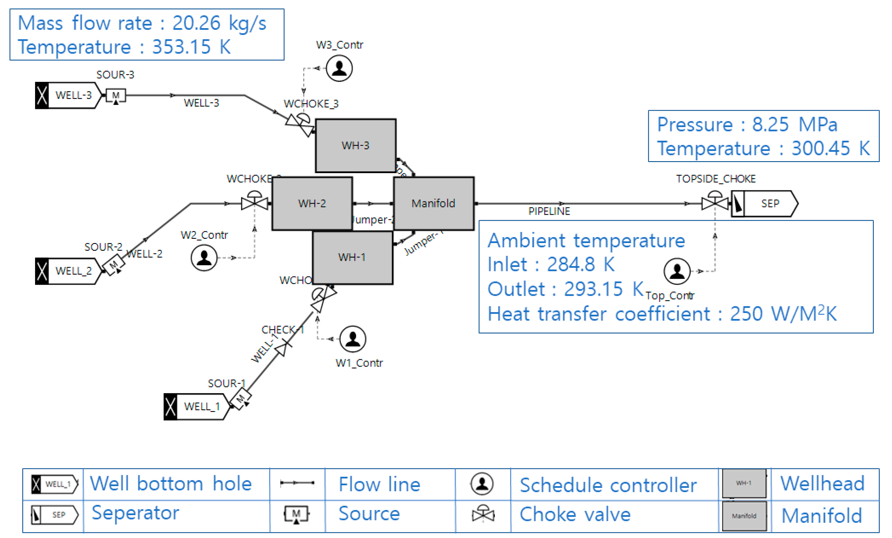
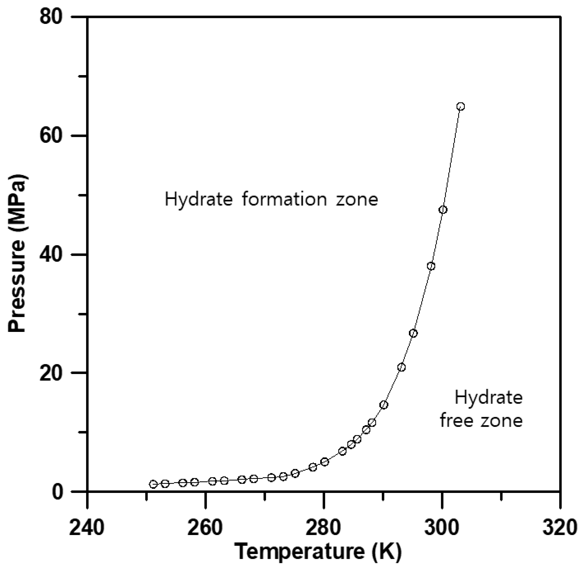
2.1. The Calculation Model of Hydrate Formation Using OLGA
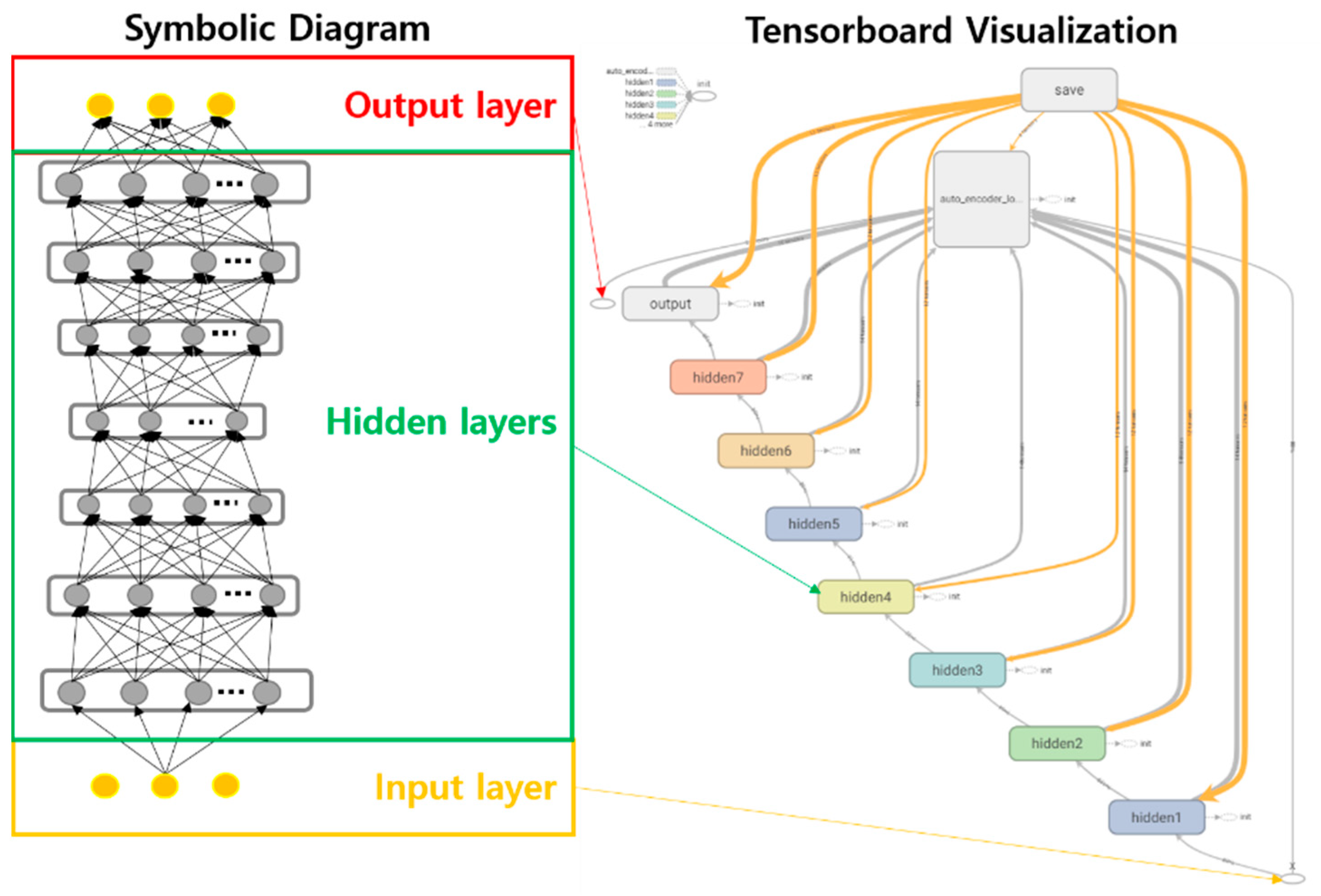
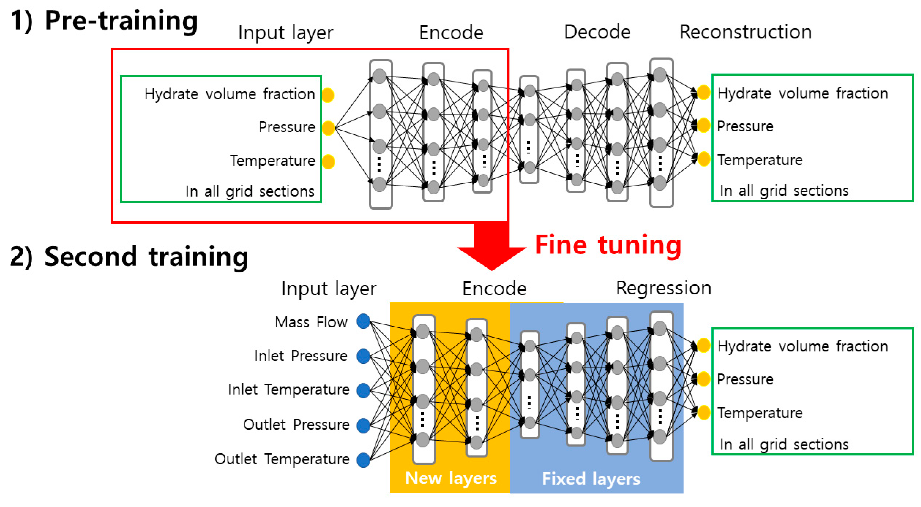
2.2. Machine Learning Using Stacked Auto-Encoder
3. Results
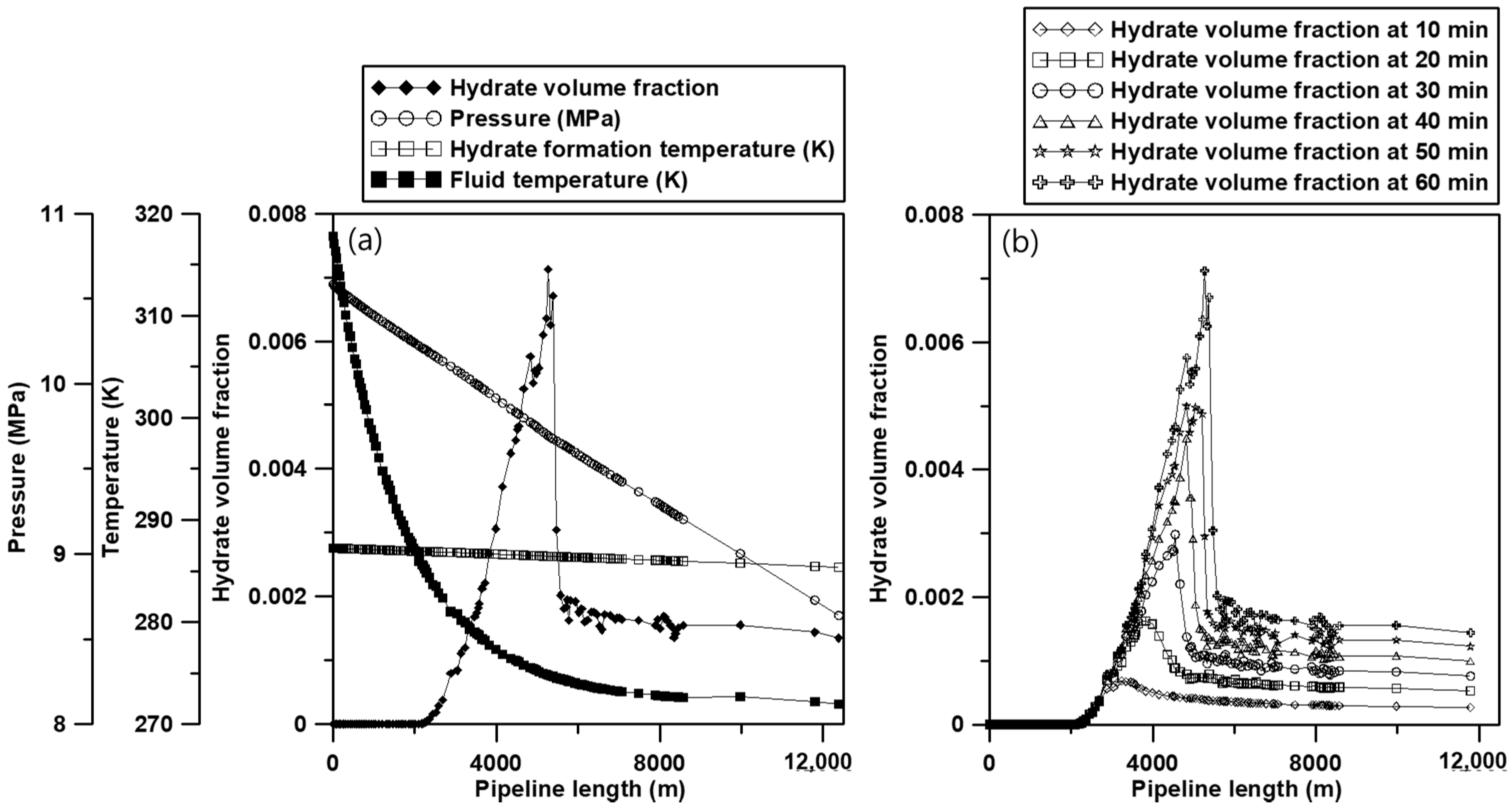
3.1. Model Construction and Base Simulation
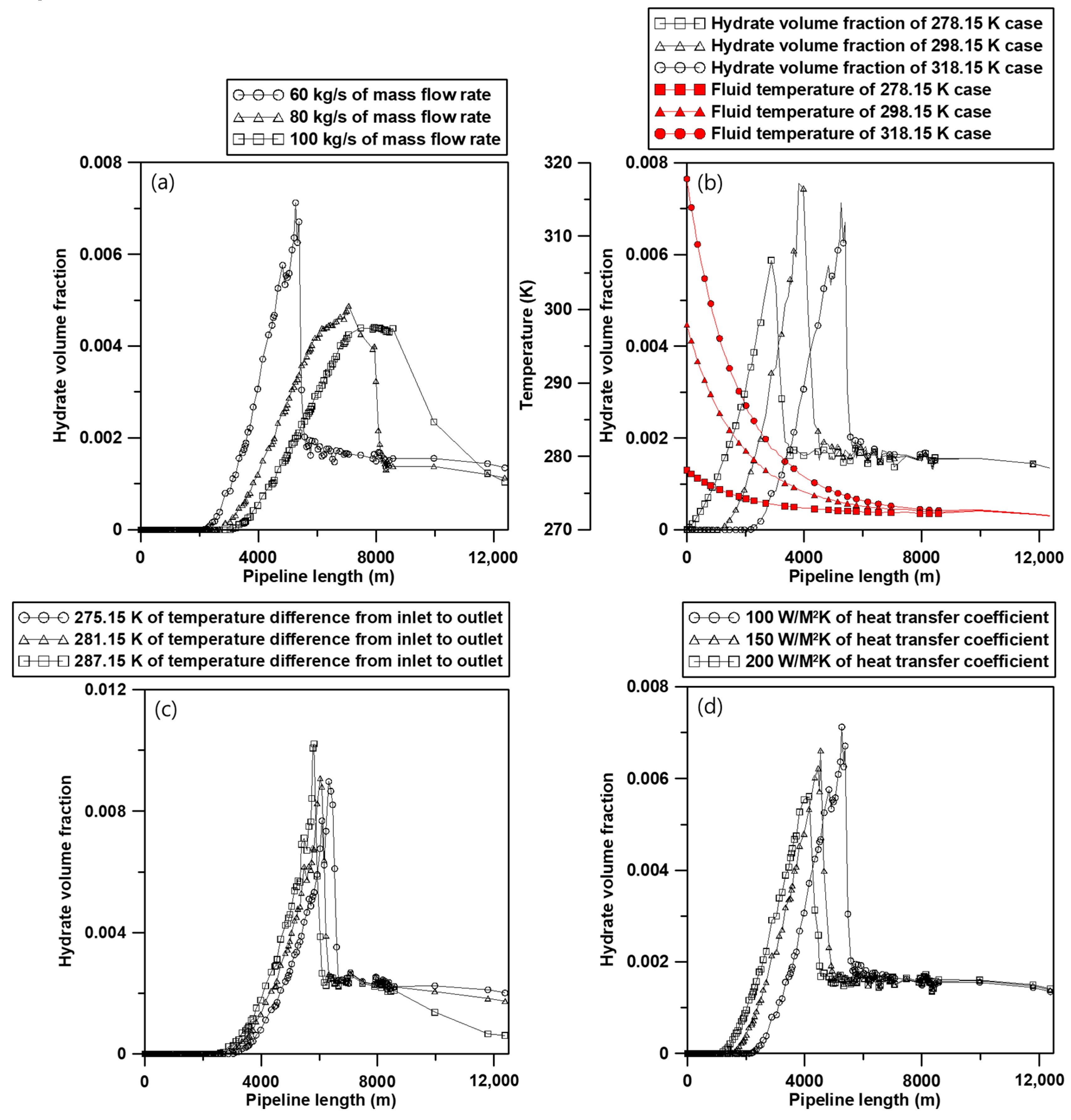
3.2. Sensitivity Study for the Generation of Learning Data
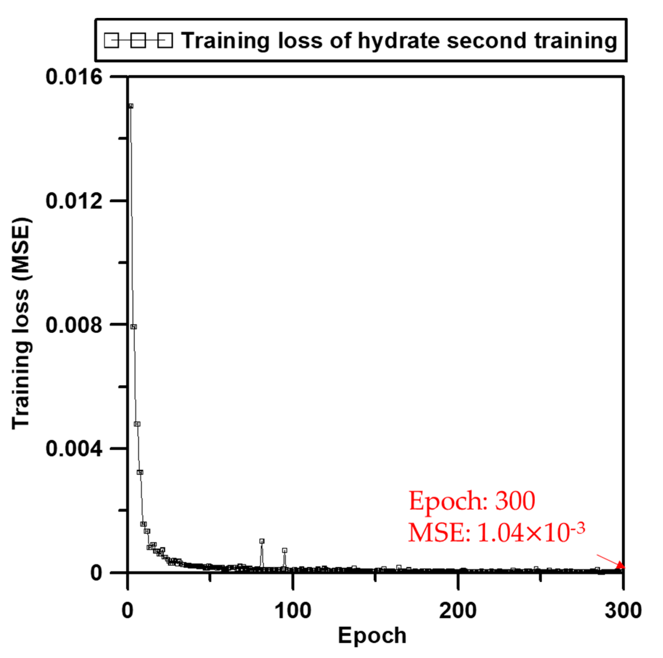
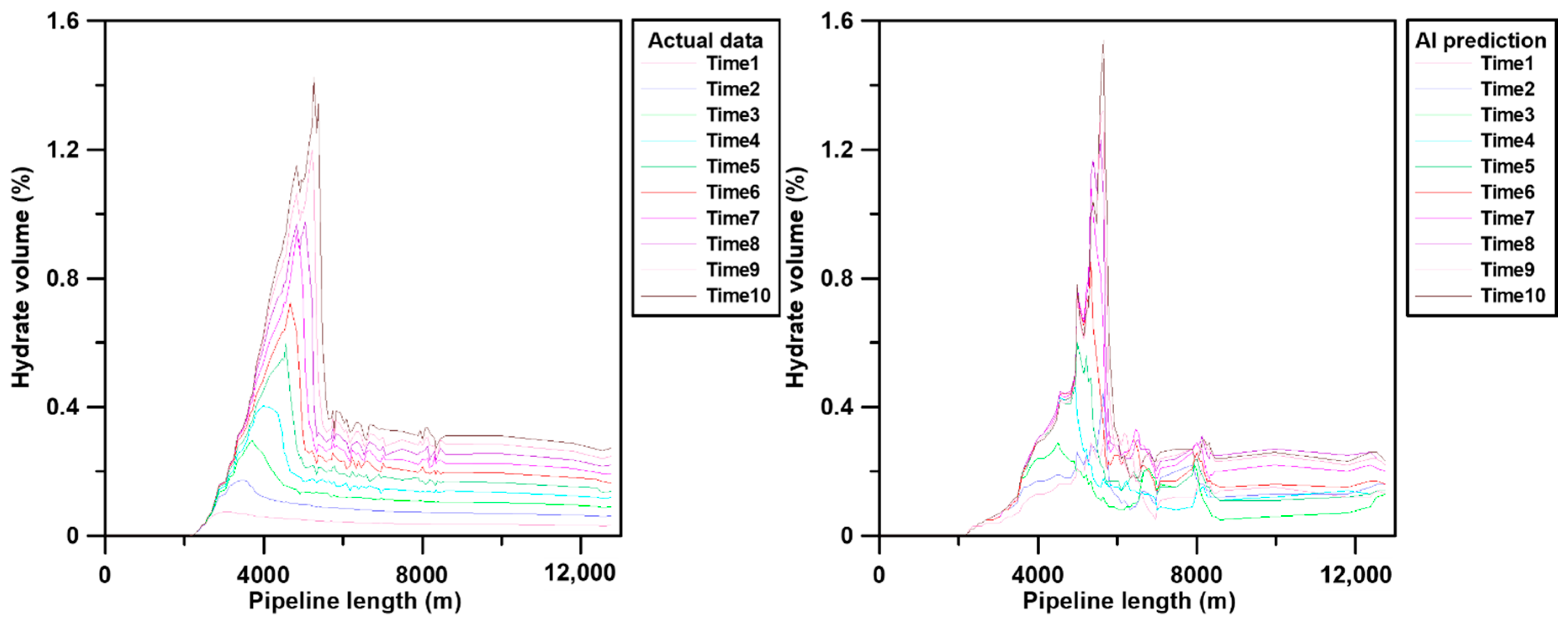
3.3. Machine Learning and Validation
4. Discussion
5. Conclusions
Author Contributions
Funding
Institutional Review Board Statement
Informed Consent Statement
Data Availability Statement
Acknowledgments
Conflicts of Interest
Nomenclature
| AI | artificial intelligence |
| ANN | artificial neural network |
| sub-cooling | |
| system temperature | |
| hydrate equilibrium temperature at system pressure | |
| mass of gas consumed per second | |
| surface area | |
| rate constant | |
| rate constant | |
| relative viscosity | |
| maximum volume fraction | |
| effective volume fraction | |
| diameter of monomer particle | |
| diameter of aggregated particle | |
| fractal dimension | |
| input | |
| reconstructed data | |
| W | weight |
| b | bias |
| SAE | stacked auto-encoder |
| MLP | multi-layer perceptron |
| LSTM | long short-term memory |
| GRU | gated recurrent unit |
| MSE | mean square error |
| SRS | simple random sampling |
| SGD | stochastic gradient descent |
| n | number of elements |
| real value | |
| predicted value | |
| learning rate | |
| weight in L2 regularization |
References
- Osaki, K. US Energy Information Administration (EIA): 2019 Edition US Annual Energy Outlook report (AEO2019). Haikan Gijutsu 2019, 61, 32–43. [Google Scholar]
- Hu, X.; Xie, J.; Cai, W.; Wang, R.; Davarpanah, A. Thermodynamic effects of cycling carbon dioxide injectivity in shale reservoirs. J. Pet. Sci. Eng. 2020, 195, 107717. [Google Scholar] [CrossRef]
- Mazarei, M.; Davarpanah, A.; Ebadati, A.; Mirshekari, B. The feasibility analysis of underground gas storage during an integration of improved condensate recovery processes. J. Pet. Explor. Prod. Technol. 2018, 9, 397–408. [Google Scholar] [CrossRef]
- Brower, D.; Prescott, C.; Zhang, J.; Howerter, C.; Rafferty, D. Real-Time Flow Assurance Monitoring with Non-Intrusive Fiber Optic Technology. In Proceedings of the Offshore Technology Conference, Houston, TX, USA, 2–5 May 2005. [Google Scholar]
- Bai, Y.; Bai, Q. Subsea Engineering Handbook; Gulf Professional Publishing: Houston, TX, USA, 2018. [Google Scholar]
- Wood, D.; Mokhatab, S. Gas monetization technologies remain tantalizingly on the brink. World Oil 2008, 229, 103–108. [Google Scholar]
- Menon, E.S. Gas Pipeline Hydraulics; CRC Press: Boca Raton, FL, USA, 2005. [Google Scholar]
- Jassim, E.; Abdi, M.A.; Muzychka, Y. A new approach to investigate hydrate deposition in gas-dominated flowlines. J. Nat. Gas Sci. Eng. 2010, 2, 163–177. [Google Scholar] [CrossRef]
- Makwashi, N.; Zhao, D.; Ismaila, T.; Paiko, I. Pipeline Gas Hydrate Formation and Treatment: A Review. In Proceedings of the 3rd National Engineering Conference on Building the Gap between Academia and Industry, Faculty of Engineering, Bayero University, Kano, Nigeria, 31 May 2018. [Google Scholar]
- Foroozesh, J.; Khosravani, A.; Mohsenzadeh, A.; Mesbahi, A.H. Application of artificial intelligence (AI) in kinetic modeling of methane gas hydrate formation. J. Taiwan Inst. Chem. Eng. 2014, 45, 2258–2264. [Google Scholar] [CrossRef]
- Tractica. Artificial Intelligence Market Forecasts; Tractica: Boulder, CO, USA, 2016. [Google Scholar]
- Mohammadi, A.H.; Belandria, V.; Richon, D. Use of an artificial neural network algorithm to predict hydrate dissociation conditions for hydrogen+water and hydrogen+tetra-n-butyl ammonium bromide+water systems. Chem. Eng. Sci. 2010, 65, 4302–4305. [Google Scholar] [CrossRef]
- Zahedi, G.; Karami, Z.; Yaghoobi, H. Prediction of hydrate formation temperature by both statistical models and artificial neural network approaches. Energy Convers. Manag. 2009, 50, 2052–2059. [Google Scholar] [CrossRef]
- El Saddik, A. Digital Twins: The Convergence of Multimedia Technologies. IEEE MultiMedia 2018, 25, 87–92. [Google Scholar] [CrossRef]
- SPT Group. OLGA 2017, User Manual, Dynamic Multiphase Flow Simulator; SPT Group: Houston, TX, USA, 2017. [Google Scholar]
- Turner, D.; Boxall, J.; Yang, S.; Kleehammer, D.; Koh, C.; Miller, K.; Sloan, E.; Xu, Z.; Matthews, P.; Talley, L. Development of a hydrate kinetic model and its incorporation into the OLGA2000® transient multiphase flow simulator. In Proceedings of the 5th international conference on gas hydrates, Trondheim, Norway, 12–16 June 2005; pp. 12–16. [Google Scholar]
- Hinton, G.E.; Zemel, R.S. Autoencoders, minimum description length, and Helmholtz free energy. Adv. Neural Inf. Process. Syst. 1994, 6, 3–10. [Google Scholar]
- Vincent, P.; Larochelle, H.; Bengio, Y.; Manzagol, P.-A. Extracting and composing robust features with denoising auto-encoders. In Proceedings of the 25th international conference on Machine learning, Helsinki, Finland, 5–9 July 2008; pp. 1096–1103. [Google Scholar]
- Bengio, Y.; Lamblin, P.; Popovici, D.; Larochelle, H. Greedy layer-wise training of deep networks. Adv. Neural Inf. Process. Syst. 2007, 19, 153. [Google Scholar]
- Vishnu, A.; Siegel, C.; Daily, J. Distributed tensorflow with MPI. arXiv 2016, arXiv:1603.02339. [Google Scholar]


| Inlet Boundary | |
|---|---|
| Mass flow rate | 60 kg/s |
| Temperature | 353.15 K |
| Outlet boundary | |
| Pressure | 8.25 MPa |
| Temperature | 300.45 K |
| Horizontal pipeline | |
| Ambient temperature | Inlet: 284.8 K Outlet: 293.15 K |
| Horizontal distance | 13,000 m |
| Heat transfer coefficient | 250 W/M2K |
| Roughness | 5.00 × 10⁻⁵ m |
| Inner diameter | 0.3174 m |
| Sections | 123 |
| Operation Constraint | Field Model | Base Case |
|---|---|---|
| Mass flow rate (kg/s) | 60 | 60 |
| Inlet fluid temperature (K) | 353.15 | 318.15 |
| Outlet pressure (MPa) | 8.25 | 8.25 |
| Outlet fluid temperature (K) | 300.45 | 300.45 |
| Inlet ambient temperature (K) | 284.8 | 273.15 |
| Heat transfer coefficient (W/M2K) | 250 | 100 |
| Parameters | Range | ||
|---|---|---|---|
| Min | Mean | Max | |
| Mass flow rate (kg/s) | 60 (base) | 80 | 100 |
| Fluid temperature (K) | 278.15 | 298.15 | 318.15 (base) |
| Difference of ambient temperature from inlet to outlet (K) | 275.15 | 281.15 | 287.15 |
| Heat transfer coefficient (W/M2K) | 100 (base) | 150 | 200 |
| Input | 615 (pre-training)/5 (second training) |
| Output | 615 |
| Learning rate | 1.00 × 10⁻⁶ |
| Batch size | 1560 |
| Epoch | 10,000 |
| Drop out | 0.6 |
| L2 regularization | 0.50 × 10⁻³ |
| Activation function | Leak relu/Tanh |
| Optimizer | Adam |
| Index | Layer 1 | Layer 2 | Layer 3 | Layer 4 | Layer 5 | Layer 6 | Layer 7 | MSE |
|---|---|---|---|---|---|---|---|---|
| 1 | 128 | 64 | 32 | 16 | 32 | 64 | 128 | 32.78 |
| 2 | 256 | 128 | 64 | 32 | 64 | 128 | 256 | 14.78 |
| 3 | 1024 | 512 | 256 | 128 | 256 | 512 | 1024 | 1.59 |
| 4 | 2048 | 1024 | 512 | 256 | 512 | 1024 | 2048 | 2.96 |
| 5 | 512 | 256 | 128 | 64 | 128 | 256 | 512 | 3.08 |
| … | … | … | … | … | … | … | … | … |
| 79 | 2048 | 1024 | 512 | 256 | 512 | 1024 | 2048 | 0.98 × 10⁻³ |
| 80 | 4096 | 2048 | 1024 | 512 | 1024 | 2048 | 4096 | 1.00 |
| Index | Layer 1 | Layer 2 | Layer 4 (Fixed) | Layer 5 (Fixed) | Layer 6 (Fixed) | Layer 7 (Fixed) | MSE |
|---|---|---|---|---|---|---|---|
| 1 | 16 | 32 | 512 | 256 | 1024 | 2048 | 1.85 × 10⁻³ |
| 2 | 16 | 64 | 1.74 × 10⁻³ | ||||
| 3 | 32 | 128 | 1.09 × 10⁻³ | ||||
| 4 | 64 | 256 | 1.12 × 10⁻³ | ||||
| 5 | 128 | 64 | 1.28 × 10⁻³ | ||||
| 6 | 128 | 256 | 1.04 × 10⁻³ | ||||
| … | … | … | … | ||||
| 79 | 256 | 256 | 1.08 × 10⁻³ | ||||
| 80 | 256 | 512 | 1.07 × 10⁻³ |
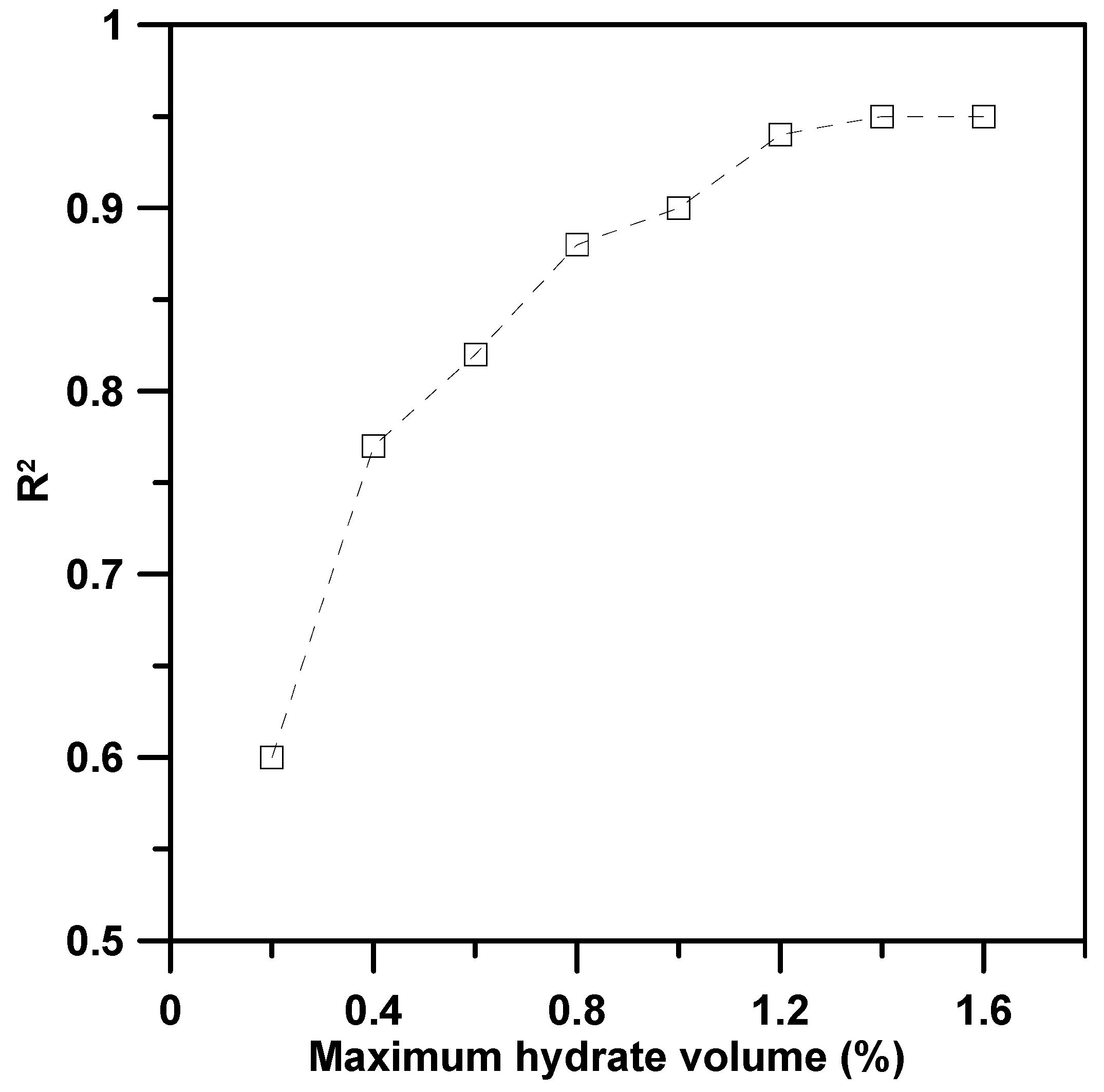
| R-Square Evaluation Result | |||
|---|---|---|---|
| Time-Series | Maximum Hydrate Volume in all Grid Sections | Pressure in all Grid Sections | Fluid Temperature in all Grid Sections |
| 6 min | 0.46 | 0.99 | 0.94 |
| 12 min | 0.59 | 1 | 0.92 |
| 18 min | 0.68 | 0.99 | 0.95 |
| 24 min | 0.78 | 1 | 0.92 |
| 30 min | 0.80 | 0.99 | 0.89 |
| 36 min | 0.84 | 1 | 0.94 |
| 42 min | 0.86 | 0.99 | 0.94 |
| 48 min | 0.87 | 0.98 | 0.89 |
| 54 min | 0.89 | 1 | 0.91 |
| 60 min | 0.95 | 1 | 0.87 |
| Average | 0.77 | 0.99 | 0.91 |
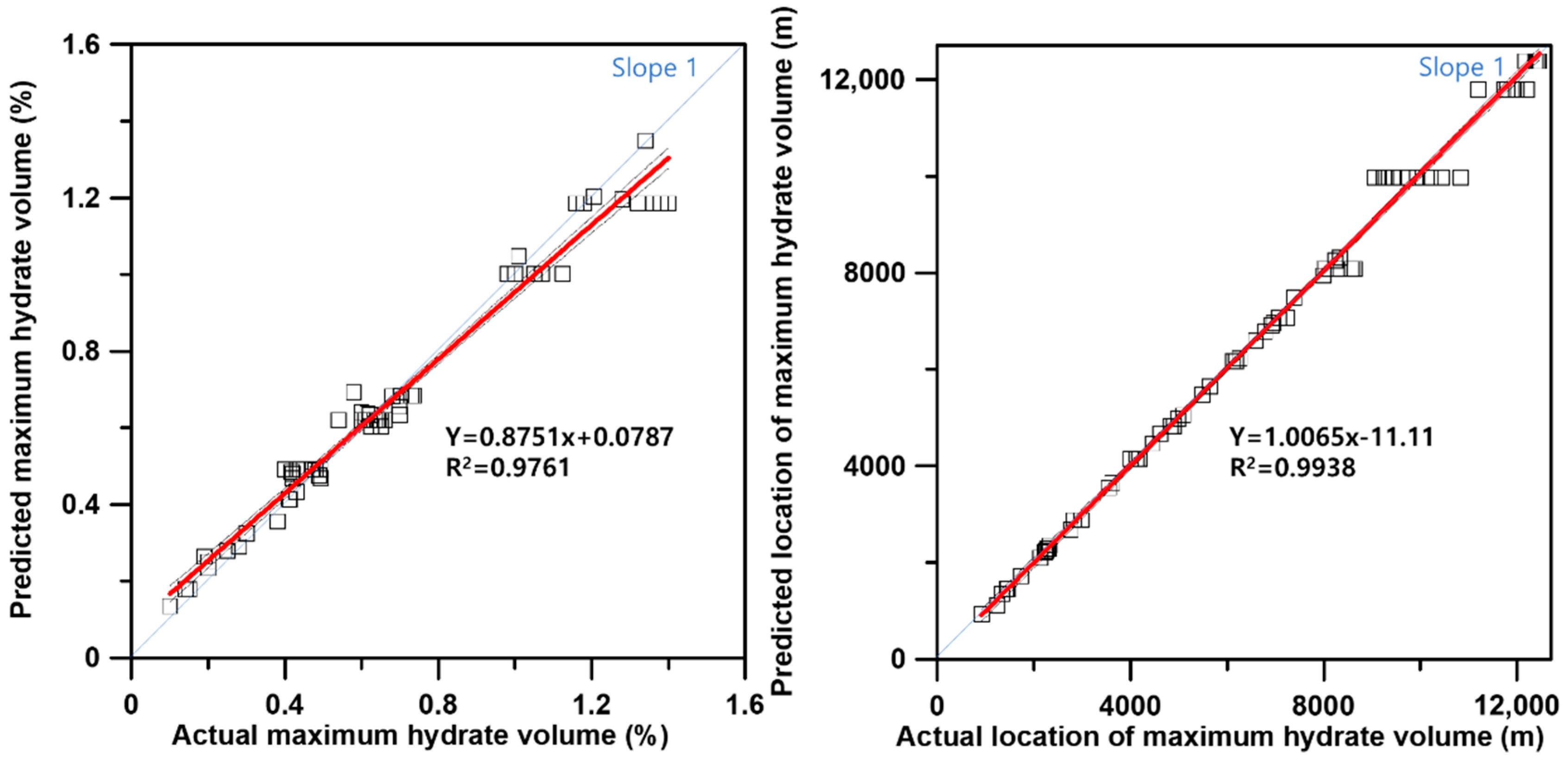
| OLGA Cases | Actual Maximum Hydrate Volume (%) | Predicted Maximum Hydrate Volume (%) | Actual Location of Maximum Hydrate Volume (m) | Predicted Location of Maximum Hydrate Volume (m) |
|---|---|---|---|---|
| Case1 | 0.41 | 0.48 | 8048 | 8082 |
| Case2 | 0.69 | 0.65 | 10,451 | 11,795 |
| Case3 | 0.31 | 0.49 | 9432 | 9970 |
| Case4 | 0.47 | 0.48 | 6781 | 6781 |
| Case5 | 0.43 | 0.49 | 11,991 | 11,795 |
| Case6 | 0.70 | 0.68 | 916 | 940 |
| Case7 | 0.41 | 0.41 | 12,171 | 12,381 |
| Case8 | 0.73 | 0.68 | 9456 | 9970 |
| Case9 | 1.06 | 1.00 | 11,939 | 11,795 |
| Case10 | 1.20 | 1.20 | 6958 | 6958 |
| … | ||||
| Case71 | 1.00 | 1.00 | 8237 | 8259 |
| Case72 | 0.48 | 0.49 | 12,201 | 11,795 |
| Case73 | 1.18 | 1.18 | 4985 | 4985 |
| Case74 | 0.98 | 1.00 | 12,413 | 12,381 |
| Case75 | 0.65 | 0.60 | 2296 | 2291 |
| Case76 | 0.73 | 0.68 | 10,435 | 9970 |
| Case77 | 0.70 | 0.63 | 8577 | 8082 |
| Case78 | 1.16 | 1.18 | 10,835 | 9970 |
| Case79 | 0.21 | 0.49 | 2823 | 2877 |
| Case80 | 0.62 | 0.62 | 8632 | 8082 |
| Average | R-square = 0.97 | MAE = 261 | ||
Publisher’s Note: MDPI stays neutral with regard to jurisdictional claims in published maps and institutional affiliations. |
© 2021 by the authors. Licensee MDPI, Basel, Switzerland. This article is an open access article distributed under the terms and conditions of the Creative Commons Attribution (CC BY) license (https://creativecommons.org/licenses/by/4.0/).
Share and Cite
Seo, Y.; Kim, B.; Lee, J.; Lee, Y. Development of AI-Based Diagnostic Model for the Prediction of Hydrate in Gas Pipeline. Energies 2021, 14, 2313. https://doi.org/10.3390/en14082313
Seo Y, Kim B, Lee J, Lee Y. Development of AI-Based Diagnostic Model for the Prediction of Hydrate in Gas Pipeline. Energies. 2021; 14(8):2313. https://doi.org/10.3390/en14082313
Chicago/Turabian StyleSeo, Youngjin, Byoungjun Kim, Joonwhoan Lee, and Youngsoo Lee. 2021. "Development of AI-Based Diagnostic Model for the Prediction of Hydrate in Gas Pipeline" Energies 14, no. 8: 2313. https://doi.org/10.3390/en14082313
APA StyleSeo, Y., Kim, B., Lee, J., & Lee, Y. (2021). Development of AI-Based Diagnostic Model for the Prediction of Hydrate in Gas Pipeline. Energies, 14(8), 2313. https://doi.org/10.3390/en14082313