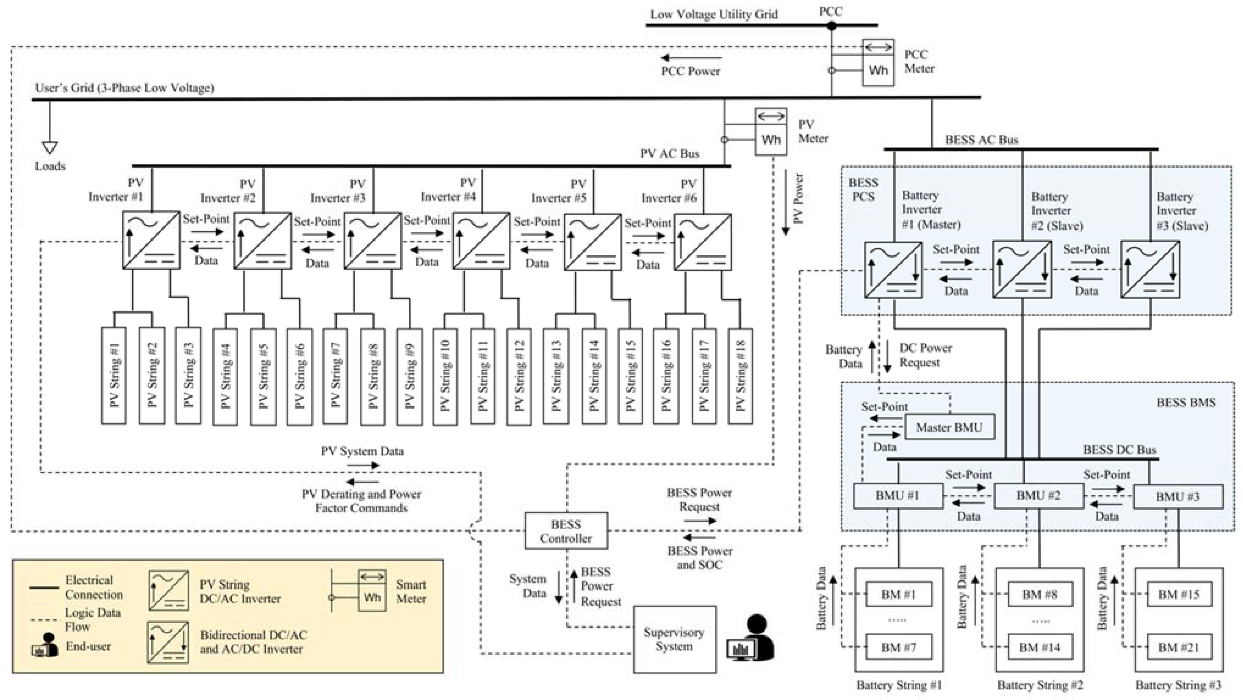
Figure 1.
Schematic layout of the PV-BESS system architecture. PV: Photovoltaic, BESS: battery energy storage system, BMS: battery management system, BM: battery module, BMU: battery management unit, PCS: power conversion system, PCC: point of common coupling, AC: alternating current, DC: direct current, SOC: state of charge.
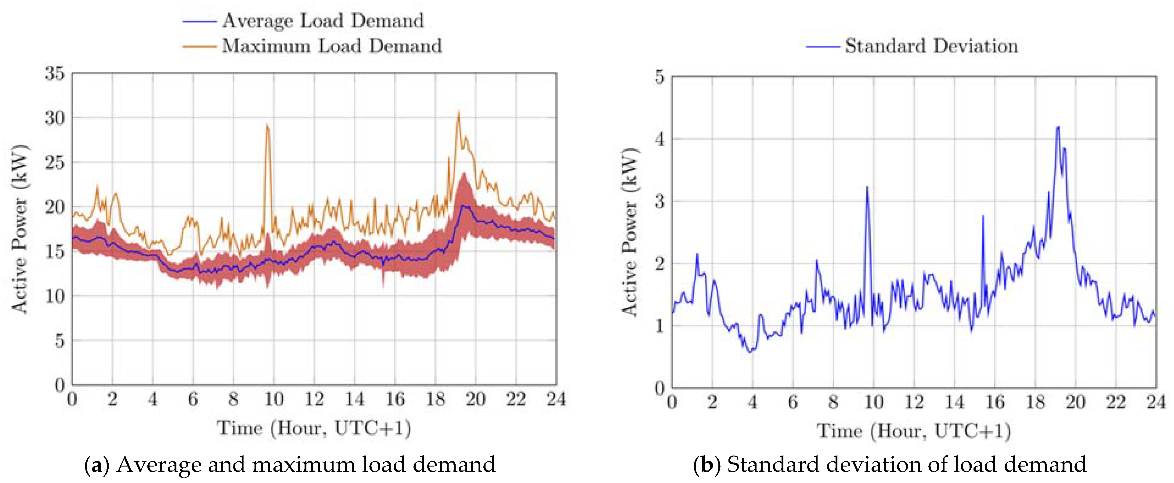
Figure 2.
Active power demand profiles of loads during May 2020. In sub-figure (a), the red area represents the standard deviation of the measurements for each -th time interval, which is reported in detail in sub-figure (b). UTC: universal time coordinated.
Figure 2.
Active power demand profiles of loads during May 2020. In sub-figure (a), the red area represents the standard deviation of the measurements for each -th time interval, which is reported in detail in sub-figure (b). UTC: universal time coordinated.
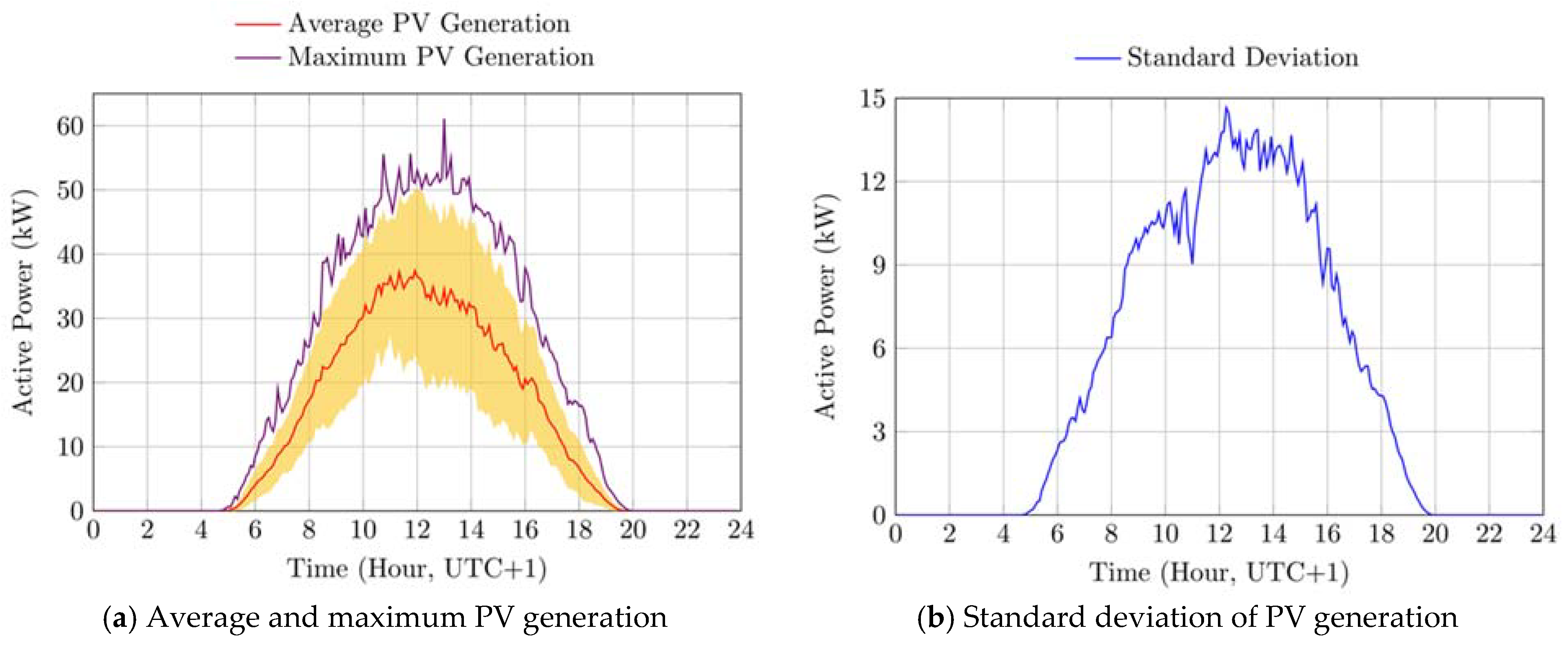
Figure 3.
Active power generation profiles of the PV system during May 2020. In sub-figure (a), the red area represents the standard deviation of the measurements for each -th time interval, which is reported in detail in sub-figure (b). UTC: universal time coordinated.
Figure 3.
Active power generation profiles of the PV system during May 2020. In sub-figure (a), the red area represents the standard deviation of the measurements for each -th time interval, which is reported in detail in sub-figure (b). UTC: universal time coordinated.
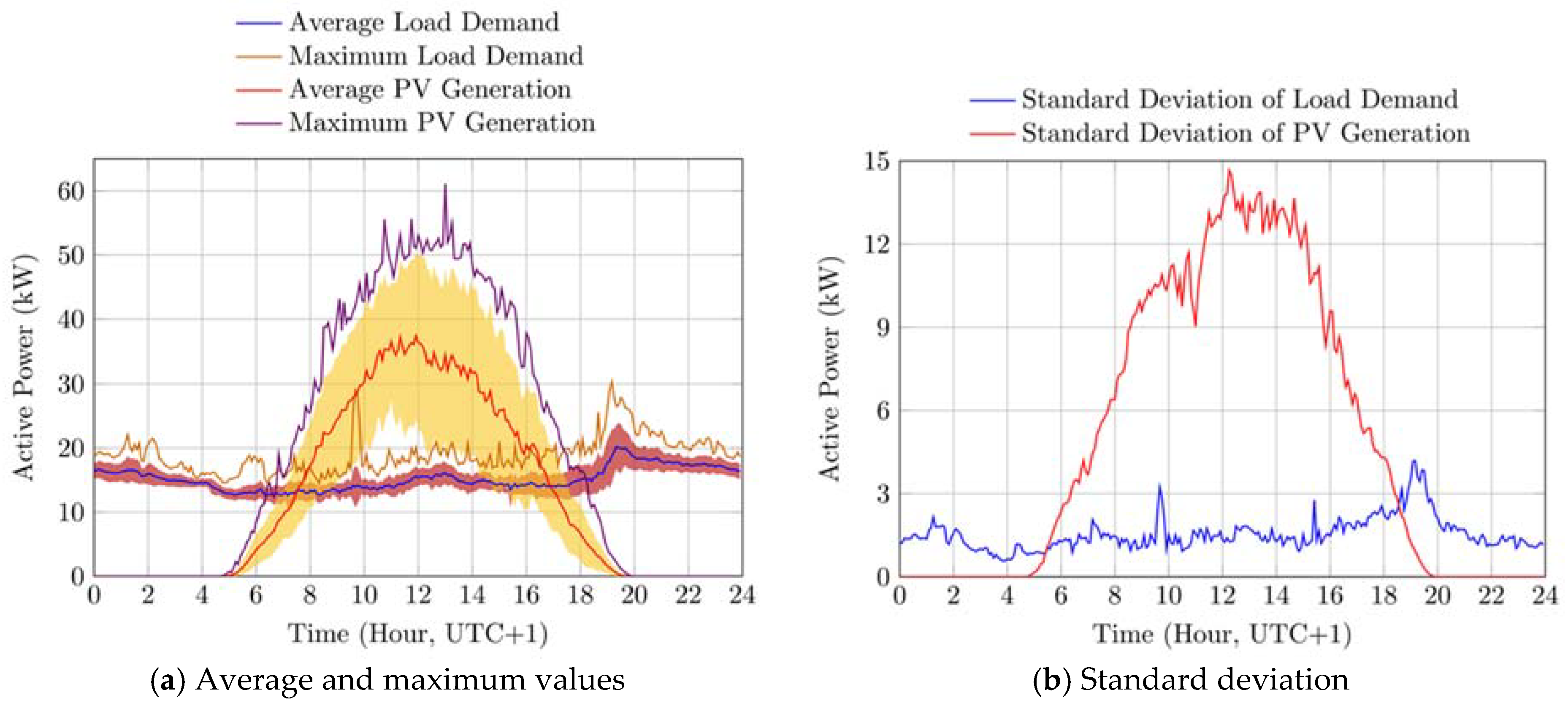
Figure 4.
Active power demand profiles of loads and PV active power generation during May 2020. In sub-figure (a), the red and yellow areas represent the standard deviation of the measurements for each -th time interval for the power demand of loads and the PV generation, respectively. The latter are reported in detail in sub-figure (b). UTC: universal time coordinated.
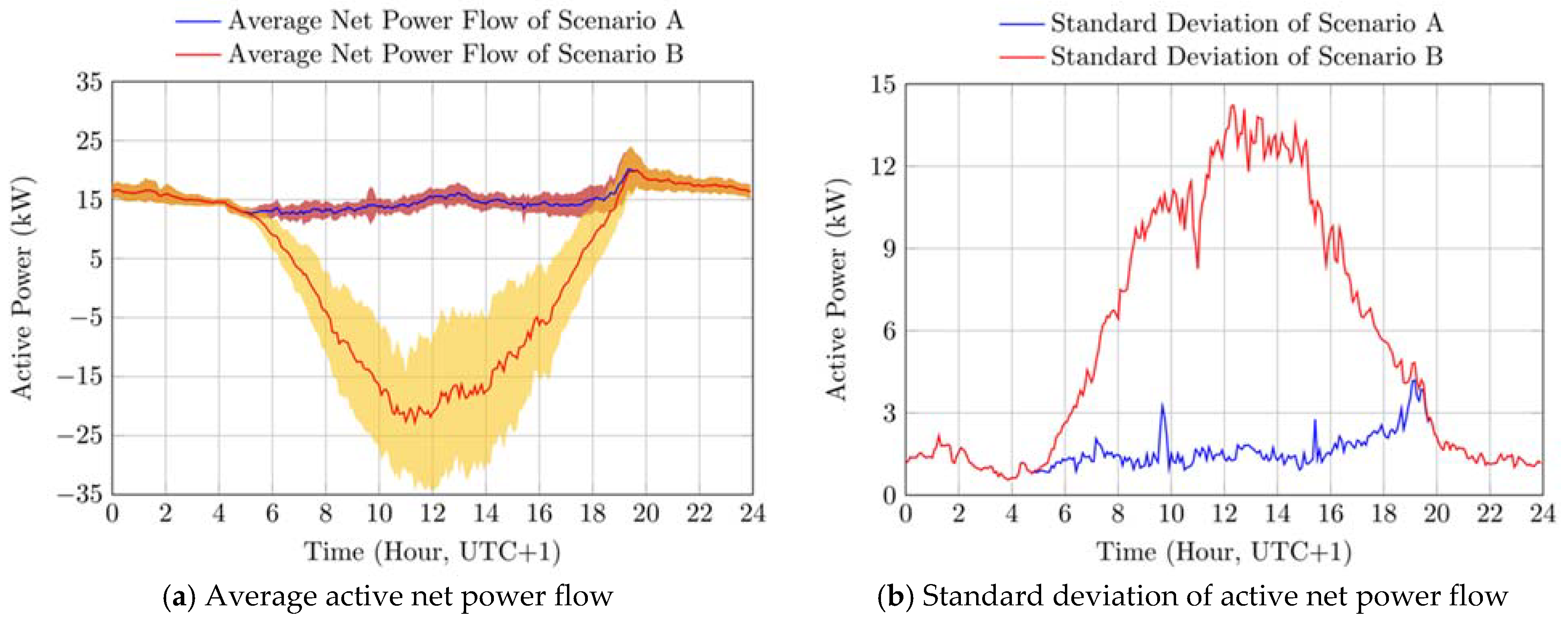
Figure 5.
Active net power flow at the PCC with the main grid for Scenarios A and B during May 2020. In sub-figure (a), the red and yellow areas represent the standard deviation of the measurements for each -th time interval for scenarios A and B, respectively. The latter are reported in detail in sub-figure (b). UTC: universal time coordinated.
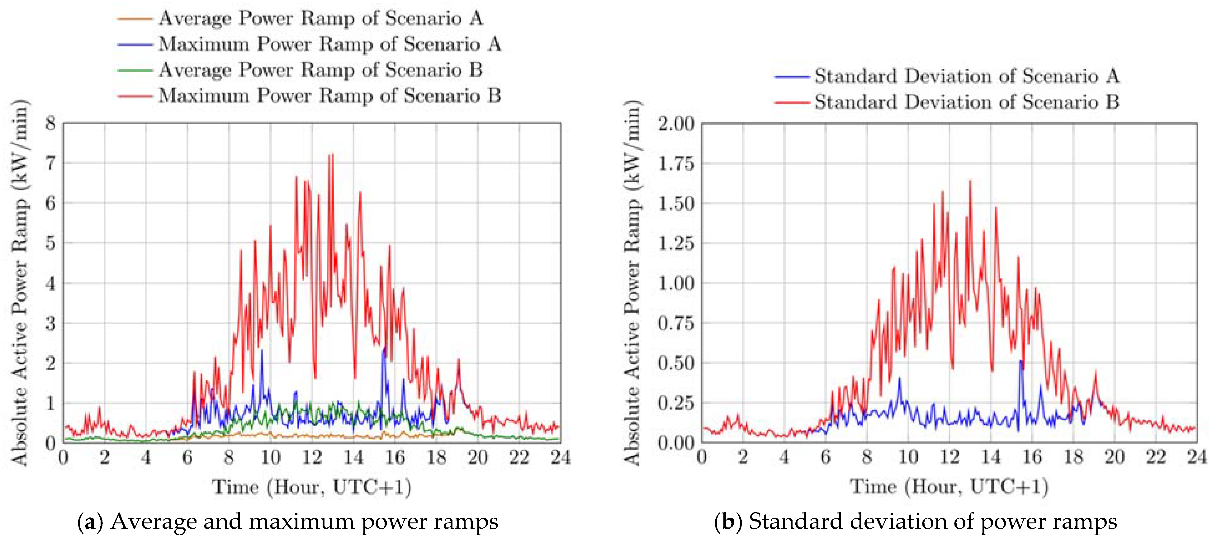
Figure 6.
Absolute power ramp of the active net power flow at the PCC with the main grid for Scenarios A and B during May 2020. In sub-figure (a), the average and maximum values of the power ramp are shown, while sub-figure (b) reports the standard deviation of the measurements for each -th time interval. UTC: universal time coordinated.
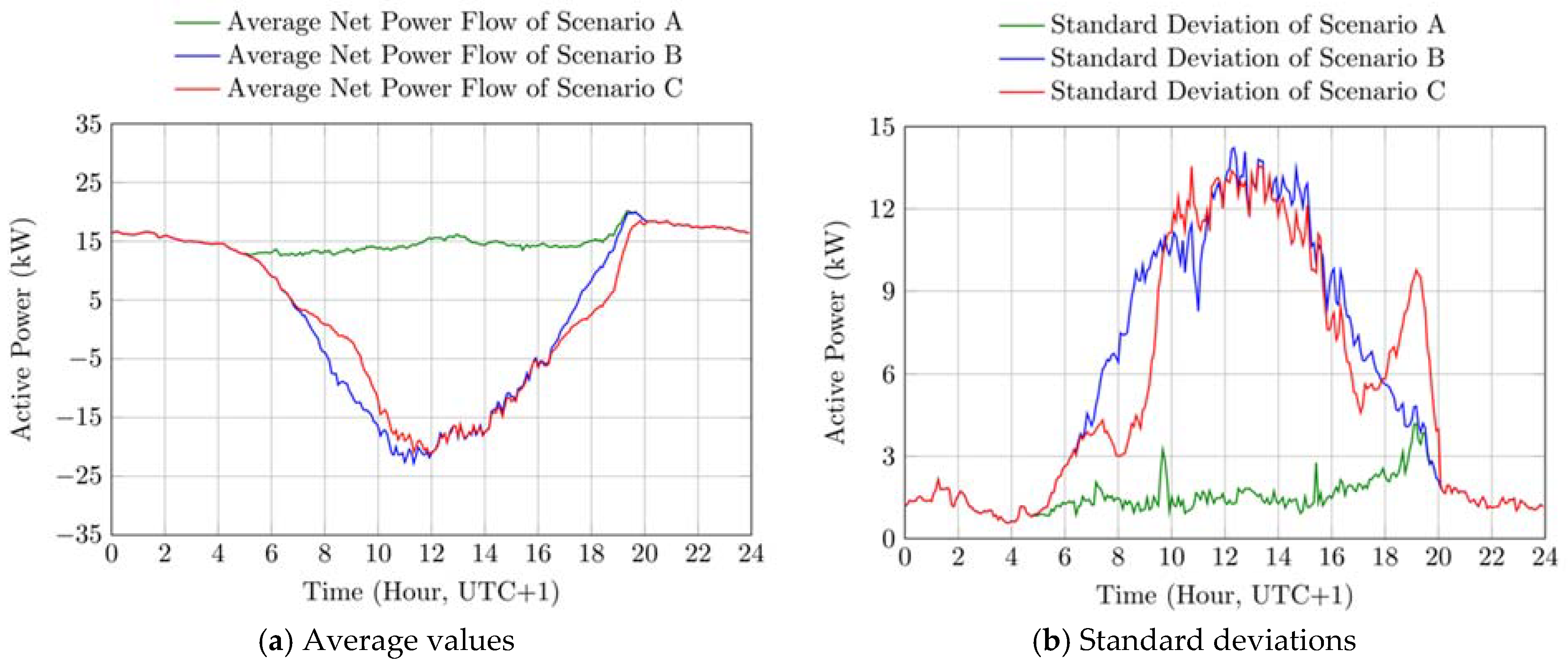
Figure 7.
Active net power flow at the PCC with the main grid for Scenarios A, B, and C during May 2020. Sub-figure (a) shows the average value of the active net power flow, while sub-figure (b) reports the standard deviation of the measurements for each -th time interval. UTC: universal time coordinated.
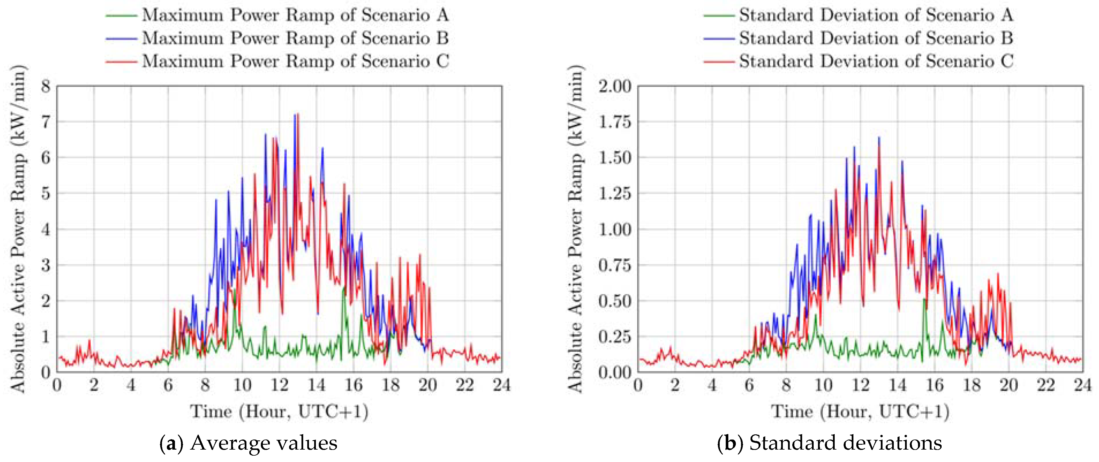
Figure 8.
Absolute power ramp of the active net power flow at the PCC with the main grid for Scenarios A, B, and C during May 2020. In sub-figure (a), the average values of the power ramp are shown, while sub-figure (b) reports the standard deviation of the measurements for each -th time interval. UTC: universal time coordinated.
Table 1.
Summary of the metrics and reference to the related equations adopted to analyze the load profiles. : average value, : standard deviation, max: maximum value.
Table 1.
Summary of the metrics and reference to the related equations adopted to analyze the load profiles. : average value, : standard deviation, max: maximum value.
| Metric | (eq.)
| (eq.)
| max (eq.) |
|---|
| Active power demand of loads during the -th time interval | (2) | (3) | |
| Daily average of the active power demand of loads | (5) | (6) | (7) |
| Daily peak of the active power demand of loads | (8) | (9) | (10) |
| Daily peak of the absolute active power ramp of loads | (13) | (14) | (15) |
Table 2.
Summary of the metrics and reference to the related equations adopted to analyze the PV profiles. : average value, : standard deviation, max: maximum value.
Table 2.
Summary of the metrics and reference to the related equations adopted to analyze the PV profiles. : average value, : standard deviation, max: maximum value.
| Metric | (eq.)
| (eq.)
| max (eq.) |
|---|
| PV active power generation during the -th time interval | (16) | (17) | |
| Daily average of the PV active power | (19) | (20) | (21) |
| Daily peak of the PV active power | (22) | (23) | (24) |
| Daily peak of the absolute PV active power ramp | (27) | (28) | (29) |
Table 3.
Summary of the metrics and reference to the related equations adopted to analyze the net power profiles at the PCC with the utility for Scenario A, i.e., without PV and storage. : average value, : standard deviation, max: maximum value.
Table 3.
Summary of the metrics and reference to the related equations adopted to analyze the net power profiles at the PCC with the utility for Scenario A, i.e., without PV and storage. : average value, : standard deviation, max: maximum value.
| Metric | (eq.)
| (eq.)
| max (eq.) |
|---|
| Active net power flow at the PCC during the -th time interval | (2) | (3) | – |
| Daily peak of grid power demand | (8) | (9) | (10) |
| Daily peak of grid power feed | | | |
| Daily peak of the absolute ramp of the active net power flow at the PCC | (13) | (14) | (15) |
Table 4.
Summary of the metrics and reference to the related equations adopted to analyze the net power profiles at the PCC with the utility for Scenario B, i.e., with PV and without storage. : average value, : standard deviation, max: maximum value.
Table 4.
Summary of the metrics and reference to the related equations adopted to analyze the net power profiles at the PCC with the utility for Scenario B, i.e., with PV and without storage. : average value, : standard deviation, max: maximum value.
| Metric | (eq.)
| (eq.)
| max (eq.) |
|---|
| Active net power flow at the PCC during the -th time interval | (32) | (34) | |
| Daily peak of grid power demand | (40) | (42) | (44) |
| Daily peak of grid power feed | (50) | (52) | (54) |
| Daily peak of the absolute ramp of the active net power flow at the PCC | (60) | (62) | (64) |
Table 5.
Summary of the metrics and reference to the related equations adopted to analyze the net power profiles at the PCC with the utility for Scenario C, i.e., with PV and storage. : average value, : standard deviation, max: maximum value.
Table 5.
Summary of the metrics and reference to the related equations adopted to analyze the net power profiles at the PCC with the utility for Scenario C, i.e., with PV and storage. : average value, : standard deviation, max: maximum value.
| Metric | (eq.)
| (eq.)
| max (eq.) |
|---|
| Active net power flow at the PCC during the -th time interval | (31) | (33) | |
| Daily peak of grid power demand | (39) | (41) | (43) |
| Daily peak of grid power feed | (49) | (51) | (53) |
| Daily peak of the absolute ramp of the active net power flow at the PCC | (59) | (61) | (63) |
Table 6.
Metrics of the load demand profile during May 2020. : average value, : standard deviation, max: maximum value.
Table 6.
Metrics of the load demand profile during May 2020. : average value, : standard deviation, max: maximum value.
| Metric | | | max |
|---|
| Daily average of the active power demand of loads (kW) | 15.16 | 0.74 | 16.28 |
| Daily peak of the active power demand of loads (kW) | 23.16 | 2.8 | 30.42 |
| Daily peak of the absolute active power ramp of loads (kW/min) | 1.19 | 0.47 | 2.38 |
Table 7.
Metrics of the PV generation profile during May 2020. : average value, : standard deviation, max: maximum value.
Table 7.
Metrics of the PV generation profile during May 2020. : average value, : standard deviation, max: maximum value.
| Metric | | | max |
|---|
| Daily average of the PV active power generation (kW). | 12.03 | 3.46 | 16.41 |
| Daily peak of the PV active power generation (kW) | 47.25 | 6.54 | 61.12 |
| Daily peak of the absolute PV active power ramp (kW/min) | 4.31 | 1.75 | 7.3 |
Table 8.
Metrics of the active net power flow profile at the PCC with the main grid for Scenario A and B during May 2020. : average value, : standard deviation, max: maximum value.
Table 8.
Metrics of the active net power flow profile at the PCC with the main grid for Scenario A and B during May 2020. : average value, : standard deviation, max: maximum value.
| | Scenario A | Scenario B |
|---|
| Metric | | | max | | | max |
|---|
| Daily peak of the grid active power demand (kW) | 23.16 | 2.8 | 30.42 | 22.85 | 2.66 | 30.16 |
| Daily peak of the grid active power feed (kW) | 0 | 0 | 0 | 32.63 | 6.14 | 46.26 |
| Daily peak of the absolute ramp of the active net power flow at the PCC (kW/min) | 1.19 | 0.47 | 2.38 | 4.27 | 1.69 | 7.23 |
Table 9.
Variation of daily peak of the grid active power demand during May 2020 between Scenario B and Scenario A. : average value, : standard deviation, max: maximum value.
Table 9.
Variation of daily peak of the grid active power demand during May 2020 between Scenario B and Scenario A. : average value, : standard deviation, max: maximum value.
| – | Absolute Difference (kW) | Relative Difference |
|---|
| −0.31 | −1.4% |
| −0.13 | −4.8% |
| max | −0.26 | −0.9% |
Table 10.
Variation of daily peak of the grid active power feed during May 2020 between Scenario B and Scenario A. : average value, : standard deviation, max: maximum value.
Table 10.
Variation of daily peak of the grid active power feed during May 2020 between Scenario B and Scenario A. : average value, : standard deviation, max: maximum value.
| – | Absolute Difference (kW) | Relative Difference |
|---|
| 32.63 | – |
| 6.14 | – |
| max | 46.26 | – |
Table 11.
Variation of daily peak of the absolute ramp of the active net power flow during May 2020 between Scenario B and Scenario A. : average value, : standard deviation, max: maximum value.
Table 11.
Variation of daily peak of the absolute ramp of the active net power flow during May 2020 between Scenario B and Scenario A. : average value, : standard deviation, max: maximum value.
| – | Absolute Difference (kW/min) | Relative Difference |
|---|
| 3.08 | 259.8% |
| 1.23 | 263.8% |
| max | 4.85 | 204.1% |
Table 12.
Metrics of the active net power flow profile at the PCC with the main grid for Scenario B and C during May 2020. : average value, : standard deviation, max: maximum value.
Table 12.
Metrics of the active net power flow profile at the PCC with the main grid for Scenario B and C during May 2020. : average value, : standard deviation, max: maximum value.
| | Scenario B | Scenario C |
|---|
| Metric | | | max | | | max |
|---|
| Daily peak of the grid active power demand (kW) | 22.85 | 2.66 | 30.16 | 22.41 | 2.64 | 30.18 |
| Daily peak of the grid active power feed (kW) | 32.63 | 6.14 | 46.26 | 30.87 | 8.48 | 46.23 |
| Daily peak of the absolute ramp of the active net power flow at the PCC (kW/min) | 4.27 | 1.69 | 7.23 | 3.86 | 1.4 | 7.23 |
Table 13.
Variation of the daily peak of the grid active power demand during May 2020 between Scenario C and Scenario B. : average value, : standard deviation, max: maximum value.
Table 13.
Variation of the daily peak of the grid active power demand during May 2020 between Scenario C and Scenario B. : average value, : standard deviation, max: maximum value.
| – | Absolute Difference (kW) | Relative Difference |
|---|
| −0.44 | −1.9% |
| −0.03 | −1% |
| max | 0.02 | 0.1% |
Table 14.
Variation of the daily peak of the grid active power feed during May 2020 between Scenario C and Scenario B. : average value, : standard deviation, max: maximum value.
Table 14.
Variation of the daily peak of the grid active power feed during May 2020 between Scenario C and Scenario B. : average value, : standard deviation, max: maximum value.
| – | Absolute Difference (kW) | Relative Difference |
|---|
| −1.76 | −5.4% |
| 2.34 | 38.2% |
| max | −0.03 | −0.1% |
Table 15.
Variation of daily peak of the absolute ramp of the active net power flow during May 2020 between Scenario C and Scenario B. : average value, : standard deviation, max: maximum value.
Table 15.
Variation of daily peak of the absolute ramp of the active net power flow during May 2020 between Scenario C and Scenario B. : average value, : standard deviation, max: maximum value.
| – | Absolute Difference (kW/min) | Relative Difference |
|---|
| −0.41 | −9.6% |
| −0.3 | −17.6% |
| max | 0 | 0% |
Table 16.
Evaluation of the prosumer’s energy balance during May 2020.
Table 16.
Evaluation of the prosumer’s energy balance during May 2020.
| Metric | Without BESS | With BESS | Absolute Difference | Relative Difference |
|---|
| 52.55% | 58.27% | 5.72% | 10.89% |
| 41.69% | 46.34% | 4.54% | 10.89% |


