Smart Balancing of Electrical Power in Germany: Fuzzy Logic Model to Simulate Market Response

Abstract

Recent EU legislation enforces the integration of European balancing markets, with harmonized products and international platforms for the procurement and activation of reserves; nonetheless, different power balancing strategies remain. The Netherlands and Belgium encourage market participants to support balancing the control block by publishing real-time information. This article refers to such concepts as smart balancing, and a market simulation tool was developed to assess the relevant market parameters for effective smart balancing. This shall contribute to the true integration of real-time balancing energy markets. The scope of the assessment of relevant market parameters was Germany, and the results showed that a pricing scheme had less impact on the results, as currently is understood by European TSOs and regulators. Moreover, the accuracy and frequency of real-time publication indicate the effectiveness of smart balancing and the associated reduction of the activation of balancing energy and associated costs. Consequently, this article proposed a road map for Germany to introduce an adapted smart balancing approach, starting with a simple traffic light.

1. Introduction

The tendency that the dispatch of electrical energy moves closer to real time is driven by opportunities for financial optimization of intra-day markets. As a consequence, power balancing becomes an ever-more interactive task where the imbalance price reflects the real-time value of energy. Meanwhile, the European legislation enforces the transition from national balancing markets to harmonized European platforms [1]. This article contributes to the discussion about the enhancement of market freedom for the purposes of designing more efficient balancing energy markets by paying special attention to an improved, market-oriented balancing approach in Germany by providing transparent imbalance pricing. Such an approach may be referred to as “self-balancing” [2] (p. 1048), “passive control” [3] (p. 102), or “passive balancing” [4] (p. 45) and is applied in The Netherlands [5] and Belgium [6]. Market participants are incentivized to deviate from their schedule to reduce the demand of balancing energy. In this article, we refer to such an approach of balancing as “smart balancing” in contrast to a balancing approach in which the market participants are left uninformed (“unaware”) about the current state of imbalance of the system. Based on simulations of a smart balancing concept designed for Germany, the results in this article show which market design choices could be made to further support efficient power balancing and establish true real-time balancing energy markets. This contributes to the European harmonization, not only for Germany, but the EU in general.

Section 1 outlines power balancing strategies and smart balancing concepts. Section 2 introduces the smart balancing model, applied scenarios for Germany, and the market response potentials considered. It describes the market design parameters regarded. Section 3 presents the results from the simulation runs including a quantification of risks and benefits and identifies worst vs. best case balancing strategies. Section 4 discusses the results and evaluates the considered market design options and policy implications. Section 5 concludes the article.

Power generation and consumption are dispatched on future, day-ahead, and intra-day markets, leading to schedules. The physical constraint of balancing generation and load is translated into the legal duty of having balanced portfolios. Therefore, market participants that represent one or a group of grid connected parties are called Balance Responsible Parties (BRPs). They financially account for any schedule deviation, which is settled with an imbalance price, individually for each 15 min Imbalance Settlement Period (ISP). As a result, unbalanced portfolios lead to financial risks of being accountable for balancing energy activated [7].

As described above, different power balancing strategies are applied in the Belgian, Dutch, and German control blocks. All countries measure the Area Control Error (ACE) in real time and activate Frequency Restoration Reserves (FRR) accordingly. Schedule deviations are settled with single imbalance pricing, meaning that every ISP is either settled with a positive or a negative price for energy deviations. This leads to the fundamental applicability of smart balancing in the first place, since participants of smart balancing concepts need to be sure that their balancing contribution is able to generate a benefit rather than additional costs. The Netherlands occasionally deviates from single pricing and changes to dual pricing in the case of counter-activation of balancing energy. This concept is referred to as “combined pricing” [8] (p. 82).

Smart balancing is a set of measures aiming at reducing the ACE and demand for balancing reserves. Principally, smart balancing refers to enabling a market response to transparent real-time imbalance pricing. Such an approach has been applied in The Netherlands since 2001 [9] and in Belgium since 2017 [10]. This article describes a smart balancing model applied for the German control block. Potential smart balancing of BRPs in Germany, their influence on the ACE, and central European system frequency are examined. Market design parameters that influence smart balancing risks and benefits are identified.

The research scopes are (i) the consequences of introducing smart balancing in Germany and (ii) market design for efficient power balancing. This article contributes to the question of which balancing market design best enables smart balancing.

2. Materials and Methods

The applied materials and methods are described to allow others to replicate and build on the results. It was assumed that BRPs optimize their behavior with the aim of maximizing their individual profit. Criteria for comparing different balancing system efficiencies are demand and costs for balancing power, as well as the impact on the European system frequency. A market design is found to be successful if it minimizes the demand and costs for balancing power.

Section 2.1 outlines the structure of the smart balancing model. Section 2.2 gives an overview of all simulated scenarios and introduces relevant market design parameter. The underlying materials are the demand and prices of balancing reserves in Germany. Historical vs. synthetic data for balancing demand and balancing energy prices are introduced. Section 2.3 describes the potential market response and the implemented fuzzy logic, which anticipates the behavior of BRPs in different market environments. Since not all the BRPs respond to market signals in the same way, the smart balancing model builds on a fuzzy logic approach. That way, it is able to reflect a “fuzzy” market response to real-time price incentives. Section 2.4 presents the validation of the smart balancing model. Section 2.5 reflects on recent studies about “under-cover” smart balancing and states the resulting limitations of the presented model.

2.1. Smart Balancing Model

The smart balancing model is implemented in Python and can be obtained by approaching the authors. Figure 1 illustrates the object-oriented model structure. On top, instances of grid elements cover calculations on system frequency (f) and activation of balancing energy according to the ENTSO-Egrid code [11]. Objects within a control block are instances of BRPs. The simulation runs carried out covered the German control block. The rest of the European synchronous zone was assumed to have a constant and balanced generation and load of 300 GW. The model can be extended by other control blocks or balancing groups.

A previous version of the model was used to simulate the week from 18 November 2019 to 24 November 2019 in a one-second resolution with field data from four BRPs [12]. The simulated behavior of the BRPs (representing industrial consumption and generation with volatile renewable sources) would have generated profit, while the demand and costs for balancing energy are reduced. The lessons learned from this field test week were used to improve and develop the model and behavior of BRPs further.

Figure 2 shows the simulation flowchart. Relevant input data from csv files are read in the initial step. Afterwards, the simulation starts with a one-minute resolution. Generation, load, and schedules are compared to calculate the ACE. Frequency and FCR activation are calculated based on a steady-state estimation, followed by aFRR activation. In scenarios with active smart balancing, the market response is calculated in the next step. The decision for mFRR activation is not based on local load-frequency control block agreements. mFRR is an optional response to critical situations, and the decision for its activation is made by the responsible Transmission System Operator (TSO) by evaluating the individual situation. mFRR is delivered in the next ISP and is included in the ACE calculation as scheduled generation. The demand and costs of aFRR and mFRR are used to calculate the imbalance price according to the current rules, enforced in 1 July 2020 [13].

2.2. Market Design Scenarios

The regarded scenarios analyze “active” smart balancing and represent different combinations of market design parameters, which have been identified in previous work [14]. In contrast to “active” smart balancing, Section 2.5 describes “under-cover” smart balancing and related limitations of the analysis.

Table 1. Overview of market design parameters.

Parameter	Variables
Availability of input	Frequent 1/min
	Traffic light (only in the case of high ACE)
Pricing scheme	Single pricing (DE)
	Combined pricing (NL)
Clearing scheme	Pay-as-bid
	Marginal with BEPP 15 min
	Marginal with BEPP 1 min
Input signals	Historic imbalance (ACE)
	Synthetic imbalance (ACE)
	Historic Merit-Order-Lists (MOLs)
	Synthetic Merit-Order-Lists (MOLs)

shows the market design parameters that are taken into account in the model. They are introduced in the following subsections.

Not all parameter combinations are of interest.

Table 2. Overview of investigated scenarios.

Scenario	Input Signals	Market Mechanisms (Clearing, Pricing)	ACE, MOL
1 no SB	Reference without SB	Pay-as-bid, single pricing	historic 2019
2 TL2	Traffic light 2 steps	Pay-as-bid, single pricing	historic 2019
3 TL5	Traffic light 5 steps	Pay-as-bid, single pricing	historic 2019
4 DE	Imbalance, price	Pay-as-bid, single pricing	historic 2019
5 NL	Imbalance, price	Pay-as-bid, combined pricing	historic 2019
6 no SB PAB	Reference without SB	Pay-as-bid, single pricing	synthetic PAB
7 DEs	Imbalance, price	Pay-as-bid, single pricing	synthetic PAB
8 NLs	Imbalance, price	Pay-as-bid, combined pricing	synthetic PAB
9 no SB BEPP15	Reference without SB	marginal, single pricing	synthetic MC
10 BEPP: 15 min	Imbalance, price	marginal, combined pricing	synthetic MC
11 no SB BEPP1	Reference without SB	marginal, single pricing	synthetic MC
12 BEPP: 1 min	Imbalance, price	marginal, combined pricing	synthetic MC

shows the simulated scenarios with their related parameter variation. The first scenario with historic data and no smart balancing served for validation of the model. Ten other scenarios were simulated to answer the research question on which market design enabled efficient smart balancing.

2.2.1. Availability of Information: Full Transparency vs. Traffic Light

Besides the Belgian and Dutch approach of making the activated FRR and the current imbalance price available to the BRPs, the alternative approach to use traffic light concepts that display fixed levels of imbalance situations was investigated. Two traffic light scenarios were defined. They represented less than full transparent approaches, but were too suitable to incentivize a market response. These traffic light concepts might be used if the fully transparent approach (as used in Belgium and The Netherlands) is regarded “too risky” or is proven to trigger market responses that cause resonance oscillations in the system imbalance.

Both traffic light approaches publish signals only in cases of higher demand of balancing energy. Concept 1 makes use of a traffic light with two increments (TL2) that distinguish between situations when the balancing energy demand exceeds 80% and when the demand exceeds 100% of contracted (automatic and manual) FRR. Concept 2 is a traffic light with five increments (TL5). It adds a signal already when the demand exceeds 60% and two more increments for high demand of over 120% and 150% of contracted FRR.

Table 3. Traffic light concepts depending on demand of contracted automatic and manual Frequency Restoration Reserves (FRR).

FRR Demand	Concept 1: TL2	Concept 2: TL5
over 60%	-	poor smart balancing
over 80%	average smart balancing	mediocre smart balancing
over 100%	good smart balancing	average smart balancing
over 120%	-	decent smart balancing
over 150%	-	good smart balancing

shows the considered increments of both approaches and the resulting smart balancing contribution of BRPs, which represent fuzzy rules (see Section 2.3) of the traffic light scenarios.

2.2.2. Single vs. Combined Pricing of Balance Responsible Parties’ Imbalance

Excluding the traffic light scenarios, all other simulated smart balancing concepts make the real-time ACE and resulting imbalance price available to BRPs. In the scenarios with single pricing, the imbalance price changes the sign only when the total sum of activated FRR has a sign shift. This approach gives an incentive for smart balancing, but does not limit the BRPs’ contribution to the ACE and can make overreactions, especially in the end of an ISP, beneficial.

In contrast to pure single pricing, the Dutch combined pricing approach was investigated. This concepts changes from single to dual pricing in any ISP with activation of both positive and negative FRR. Dual imbalance pricing punishes all schedule deviations. Therefore, combined pricing prevents the misplaced incentive of pure single pricing at the end of an ISP.

2.2.3. Clearing of Activated Frequency Restoration Reserves

The costs for balancing result from the ACE in combination with the submitted energy bids for FRR. All bids are ordered by price and together form a Merit-Order-List (MOL). The comparison of the German balancing energy clearing scheme “pay-as-bid” vs. marginal clearing is of interest, because Germany will introduce marginal clearing in 2021 due to the European Electricity Balancing (EB) Regulation [1].

Pay-as-bid leads to an optimal bidding strategy where bids include mark-ups leading to high prices in the repeated auction setting [15]. Bidders have an incentive to include a mark-up reflecting their competitive position, but observed high prices for energy bids in Germany are also caused by the limited set of suppliers and the auctions being repeated on a regular basis [16]. Besides the energy bid, also the power bid (respectively capacity bid) and related procurement mechanisms influence the bidding strategy [17], but are not reflected by the presented model.

Marginal pricing, on the other hand, leads to underbidding of energy production costs [18].

Marginal clearing does not incentivize bidders to reveal their true costs in their bids, but to understate them for a good merit-order position. In contrast, considering the observed extreme energy bids in Germany, we assumed that substantial mark-ups were included when pay-as-bid was applied. The corresponding costs are higher than the costs of paying the uniform price to all activated BRPs at a low ACE. On the other hand, marginal pricing leads to high costs with high ACE. The resulting incentives for smart balancing should lead to less occurrences of high ACE in a marginal clearing market. Figure 3 illustrates these assumed correlations, which are subject to the discussion in Section 4.

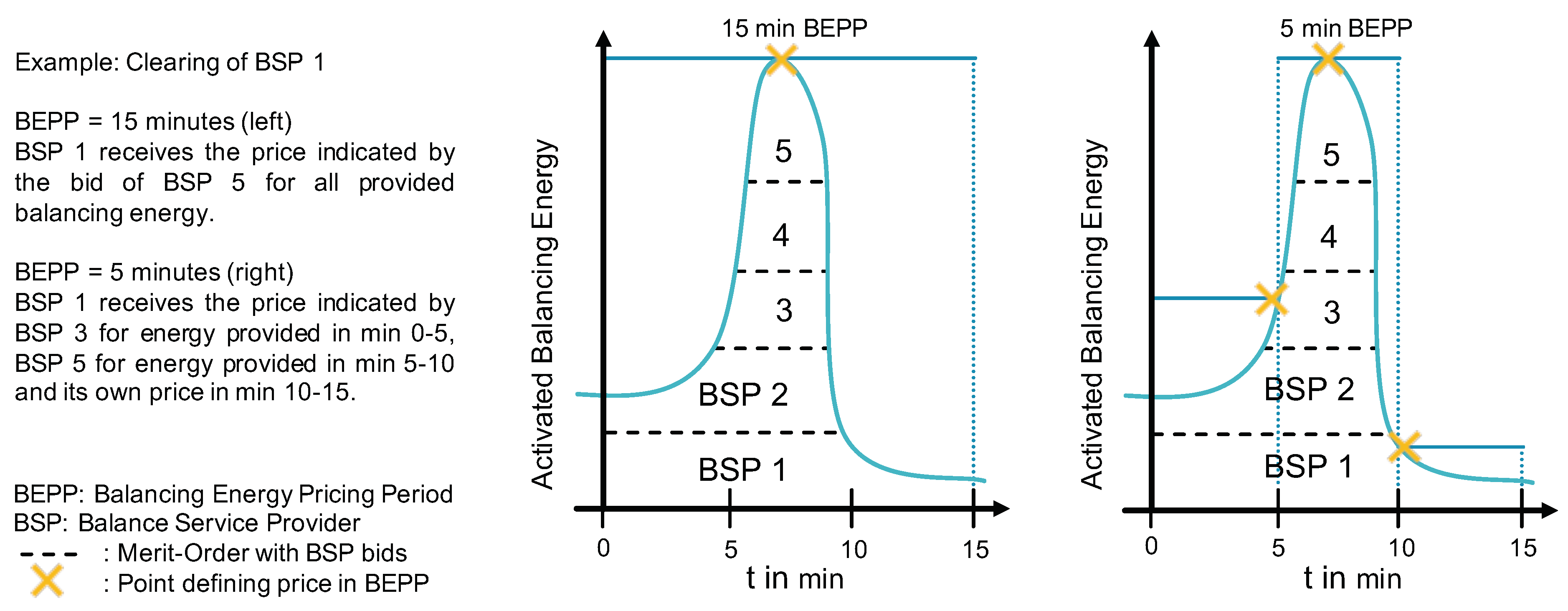
The Balancing Energy Pricing Period (BEPP) in a marginal clearing setup is usually equal to the ISP. In the context of the new EB Regulation, a change from pay-as-bid to marginal pricing with a BEPP of 15 min vs. a BEPP of 1 min is of interest. Figure 4 illustrates and explains the BEPP with an example. A small BEPP can prevent high costs for FRR in the case of high ACE, as the marginal price is updated more frequently. A 15 min BEPP and a 1 min BEPP were compared in this study to investigate their influence on smart balancing. Since the simulations with historic data in Section 3 showed that combined pricing is a useful instrument for successful smart balancing as practiced in The Netherlands, this choice remained.

2.2.4. Historic vs. Synthetic Area Control Error and Merit-Order-Lists

As shown in Table 2, five investigated scenarios used historic data from the year 2019, and six scenarios used synthetic data. In scenarios with historic data, market mechanisms and flexibility providers face the historic ACE and MOLs. This includes events with high imbalances in June 2019 and might showcase the advantage of smart balancing during these events. The considered data to (re-)build the historic ACE in a 1-min resolution were the automatic Frequency Restoration Reserves (aFFR) in a 1-s resolution and the manual Frequency Restoration Reserves (mFRR) and the emergency reserves both in a 15-min resolution [19]. The total ACE would also include the German contribution to the International Grid Control Cooperation (IGCC), but this contribution was neglected since it did not lead to an activation of FRR and even reduced the demand for balancing energy in other control blocks [20]. The historic ACE was only used for reference and for the four scenarios with the pay-as-bid clearing.

The reference scenario of 2019 served for calibration and validation in the attempt model the German energy market as it is. The current situation in Germany can be defined as a “no active smart balancing”, “single pricing”, and “pay-as-bid clearing” scenario.

Nevertheless, the historic data did include “under-cover” smart balancing (see Section 2.5), and the MOLs were determined in a pay-as-bid clearing scheme. Input data including synthetic ACE and MOLs allowed generating reasonable scenarios for market design comparison.

The ACE with pay-as-bid (PAB) clearing was defined to fluctuate between 1.1 GW and −1.1 GW with a random variation between −40 MW and 40 MW, calculated by Equation (1).

$$sAC{E}_{PAB}=1.1\mathrm{GW}\ast sin(T=12.1h)+40\mathrm{MW}\ast rand(-1,1)$$

(1)

Marginal Clearing (MC) prevents high ACE by higher related costs, as illustrated in Figure 3. Therefore, the ACE with marginal clearing is defined to fluctuate between 1 GW and −1 GW with a random variation between −40 MW and 40 MW, calculated by Equation (2).

$$sAC{E}_{MC}=1\mathrm{GW}\ast sin(T=12.1h)+40\mathrm{MW}\ast rand(-1,1)$$

(2)

Scenarios with synthetic data used two different MOLs, depending on the clearing scheme and resulting bidding behavior (see Section 2.2.3). The total average costs with pay-as-bid vs. marginal clearing of balancing energy without smart balancing were assumed to be equal, leading to the MOLs introduced in

Table 4. Synthetic Merit-Order-Lists (MOLs) for smart balancing simulation.

Reserve Type	Pay-as-Bid Clearing
	Power	Price
positive aFRR	1700 MW in 100 MW steps	30 to 350 EUR/MWh in 20 EUR/MWh steps
negative aFRR	−1800 MW in 100 MW steps	−10 to 330 EUR/MWh in 20 EUR/MWh steps
positive mFRR	800 MW in 100 MW steps	110 to 250 EUR/MWh in 20 EUR/MWh steps
negative mFRR	−600 MW in 100 MW steps	80 to 220 EUR/MWh in 20 EUR/MWh steps
	Marginal clearing
	Power	Price
positive aFRR	1700 MW in 100 MW steps	30 to 190 EUR/MWh in 10 EUR/MWh steps
negative aFRR	−1800 MW in 100 MW steps	−10 to 160 EUR/MWh in 10 EUR/MWh steps
positive mFRR	800 MW in 100 MW steps	110 to 180 EUR/MWh in 10 EUR/MWh steps
negative mFRR	−600 MW in 100 MW steps	80 to 130 EUR/MWh in 10 EUR/MWh steps

.

2.3. Market Response with Fuzzy Logic

This section introduces the implemented flexibility providers. They respond to real-time signals, if the imbalance price covers their marginal costs. Energy exchange resulting from smart balancing contributions, as well as the resulting profit were calculated to analyze their impact. BRPs were defined within the control block, and their behavior was anticipated with fuzzy logic. They reacted to the ACE and the imbalance price of the control block.

Information relevant for financial optimization at minimized risk was identified and defined as input parameters for the fuzzy logic via fuzzy rules. Results were investigated regarding the financial benefit of BRPs and their contribution to system stability.

2.3.1. Potential Market Response

The considered technologies that have a (smart) balancing potential are shown in

Table 5. Assumption for profit optimization parameters of BRP based on the German imbalance price (Ausgleichs-Energie-Preis (AEP)) and the day-ahead auction price for electrical energy ($d{a}_{price}$).

Technology	Potential Up/Down (MW)	Marginal Costs Up/Down (Euro)
Aluminum electrolysis	281/-	$AEP-d{a}_{price}>100$/-
Cement raw mill	116/50	$AEP-d{a}_{price}>100$/$AEP<10$
Cement mill	265/113	$AEP-d{a}_{price}>100$/$AEP<10$
Amalgam chlorine electrolysis	114/72	$AEP-d{a}_{price}>100$/$AEP<10$
Membrane chlorine electrolysis	359/227	$AEP-d{a}_{price}>100$/$AEP<10$
Electric arc furnace (Steel)	753/-	$AEP-d{a}_{price}>250$
Polisher in paper production	207/46	$AEP-d{a}_{price}>100$/$AEP<10$
Refiner in paper production	105/23	$AEP-d{a}_{price}>100$/$AEP<10$
Solar and wind (Build 2017, 2018)	-/dynamic	-/$AEP<-EEGbonus-40$
Gas fired power plants	dynamic/dynamic )	$AEP>50$/$AEP<0$

. Furthermore, their assumed flexibility potential and (smart) balancing logic are shown. The technologies belong to three different categories. Industrial processes represent the currently available flexibility from Demand Side Integration (DSI). Based on a recent analysis [21], it can be assumed that only the stated DSI technologies are able to contribute a market response without further investments. Renewable energy technologies have the possibility to respond to external signals and ramp down power generation. Only generation plants installed in the year 2017 and 2018 that fall under the “Markt-Prämien-Modell” were considered, because they face an incentive for smart balancing.

2.3.2. Profit Estimation of Smart BRPs

Smart balancing was determined by the given market design and the related opportunities to generate revenues. Figure 5 illustrates all steps around the fuzzy logic for the calculation of the respective smart balancing contribution for BRPs and assets with smart balancing potential. The net margin was derived from the imbalance price, which is the incentive for smart balancing and therefore mandatory to be considered. It quantifies the potential specific revenue and therefore the willingness to deviate from the BRP’s schedule. The calculation logic differed for all simulated BRPs, as stated in Table 5. The imbalance prices and the implemented marginal costs of BRPs led to individual net margin values.

The “End of ISP” box illustrates the test, if the end of an ISP is reached, implemented by Equation (3). If T is equal to 14, the formula returns true and sets the smart balancing of the regarded BRP to zero (“No SB” box).

$$(T-14)modulo15=0$$

(3)

The “Profit” box illustrates the consideration, if smart balancing would generate revenues, tested by Equation (4). If the marginal costs are higher than the imbalance price, the smart balancing of the regarded BRP was set to zero (“No SB” box).

$$AE{P}_{T-1}>marginalcosts$$

(4)

The “fuzzy logic” box represents the “fuzzy” behavior of BRPs, described in Section 2.3.3. The time step, the current smart balancing contribution, and the technical potential were used as the input. In addition, the ACE or the activated FRR quantified the absolute revenue potential. A high imbalance enabled a high smart balancing participation and set an upper limit, since a market response larger than the occurring imbalance could change the sign of the imbalance price and therefore cause monetary losses. Counter-activation of FRR immediately changed the sign of the imbalance price in the case of combined pricing, and the ACE was used as the fuzzy input. In the case of pure single pricing, the sign only changed if the counter-activation was higher than the initially activated FRR over 15 min, and the sum of activated FRR was used as input.

The “Risk” box illustrates a test, if the resulting behavior would reduce the ACE by over a third of its value, tested by Equation (5). If this was true, the “Limit SB” box reduced the smart balancing accordingly. The limit was chosen in order to avoid fast response in case of high incentives.

$$sb{P}_{T+1}>ACE/3$$

(5)

The “Sufficient ramp” box illustrates the last test, if the resulting behavior can be realized with the underlying technology, tested by Equation (6). If this was false, the “Limit SB” box reduced the smart balancing according to the technical limit.

$$sb{P}_{T+1}-sb{P}_T<ramp$$

(6)

2.3.3. Fuzzy Behavior of Smart BRPs

Besides the basic consideration of profit and risks as shown in Figure 5, the further decision on how much of the smart balancing potential was activated was simulated using fuzzy logic. Fuzzy logic was first introduced in 1965 [22] for complex control of systems where behavioral aspects of multi-criteria decision making are anticipated. The applied Mamdani-type fuzzy inference was based on rules with linguistics, which was first introduced in 1975 [23]. The implementation was realized with the Python library scikit-fuzzy, which is a fuzzy logic toolkit for SciPy [24]. The centroid method was used as the defuzzification technique.

A previous version of fuzzy logic was used to anticipate the behavior of BRPs in changing market environments and a 1 GW imbalance test case [25]. The new version introduced in the following was extended to represent BRPs market response according to a situation in which all market participants would join smart balancing. It was better scaling.

Table 6. Overview of parameters investigated for market response modeling.

Parameter	Parameter Range	Unit	Explanation
Imbalance	−1001 to 1001	MW	Quantifies absolute revenue potential, global balancing limit
Ratio	0 to 600	%	Quantifies if Flexpotentialis higher ACE
			individual balancing limit
Time	0 to 15	min	Indicates probability of changing sign of imbalance price
			actual billing period (ISP)
Imbalance sign	0 or 1	-	Indicates that further SB contribution would increase imbalance
Smart balancing	0 to 100	%	Fuzzy output for smart balancing power calculation

gives an overview about the considered input parameters for the fuzzy logic and implemented range.

These parameters were chosen since they covered the information needed to enable a reasonable balancing behavior, as simple as possible, as complex as necessary. Smart balancing is a product of activated balancing energy, time, and imbalance price.

To identify ISPs with financial opportunities, information about the imbalance price, the imbalance height, as well as the remaining time of the ISP as an indicator for the risk of loosing money in case of a changing sign of the imbalance price within the ISP needed to be regarded.

The time was used as an indicator for the risk of an changing imbalance sign. The earlier within the actual billing period we are, the greater the risk of a changing sign. For the fuzzy logic, the ISP of 15 min was therefore split into three uniform five-minute intervals “early”, “middle”, and “late”.

Since balancing was conducted by several BRP at the same time, an additional parameter to anticipate the behavior of other participants was introduced. This was needed to scale the market response and reduce overshoots. For this purpose, the power contribution was added. The power contribution quantified the individual contribution to the system state. A high power contribution scaled the markets response to a high value, and a low contribution lowered it. This set an individual balancing limit to prevent overshooting and profit loses.

Fuzzy membership functions and fuzzy rules are listed in Appendix A.

2.4. Validation via Correlation Factor

Correlation factors were used as an indicator for the quality of the simulation. The rules for mFRR activation were tuned to optimize the correlation between the simulated and the historic mFRR activation, resulting in the following “best-fit” approach:

• Check average value of ACE over the first five minutes of any ISP
• Activation of mFRR in case the average ACE exceeds 37%/36% of procured (pos./neg.) aFRR
• Activation of mFRR, which reduces the demand to 41%/37.5% of available (pos./neg.) aFRR

The results from the validation scenario with historic ACE, no smart balancing’, and 525,600 time steps at 1-min resolution was used to generate data with 35,040 time steps at 15-min resolution, representing the format of the historic data from ENTSO-E Transparency [26]. The activated balancing energy and related costs, as well as the imbalance price were compared to the historic values.

Table 7. Correlation factors between historic values [26] and time series resulting from the validation scenario “1 no smart balancing”.

Parameter	aFRR	mFRR	AEP
Energy up	0.86	0.58	-
Energy down	0.89	0.53	-
Costs up	0.69	0.57	-
Costs down	0.72	0.32	-
Price	-	-	0.52

shows the correlation factors between historic values and time series resulting from the 2019 validation scenario. The comparison demonstrated that the validation scenario led to results with middle to high correlations, and only costs for downwards mFRR had a small correlation. The aFRR energy and costs values had a good quality. The mFRR energy values and costs for upwards mFRR had a middle quality. The quality of mFRR values could be traced back to the manual process in reality vs. a static decision making in the model. The resulting imbalance price had a middle correlation. On the other hand, the research scope was not to reproduce historic energy and cost values, but to apply a suitable environment to simulate different market environments and smart balancing behavior. For that reason, the model was considered to enable valid analysis.

The validation scenario was used as the benchmark “1 no smart balancing” for the four smart balancing simulations with historic data and pay-as-bid clearing. The finding error rate and accuracy of all smart balancing scenarios were not only based on the above-stated correlation factors, but were mainly driven by the accuracy of the assumed smart balancing behavior. Quantification of this accuracy made field tests necessary. The finding error rate and accuracy should be analyzed in future work.

2.5. Limitations and “Under-Cover” Smart Balancing

Smart balancing, generally said, is the market response to the ACE and the resulting imbalance price. The two input signals correlate, depending on the market design and costs for balancing energy. Germany applies single pricing, but does not allow for schedule deviations [7].

This paradox leads to “under-cover” smart balancing in Germany, which could be shown in previous studies: An equilibrium in the market of supply and demand in real-time was identified, where the system imbalance declined by 2.8 MW per 1 EUR/MWh increase in the imbalance price. According to the analysis of historic data (12.06.18 to 29.09.2019), strategic schedule deviations reduced the German ACE by about 20% [27]. This benefit was reached mainly by strategic bidding at intra-day markets where BRPs took all available information into account for an anticipation of the ACE in the next ISP. On the other hand, such a price responsiveness could lead to overreactions of the market [28]. Another evidence-based study claimed that the activation of manual Frequency Restoration Reserves (mFRR), which indicates high ACE and an expensive imbalance price, leads to ”under-cover“ smart balancing [29]. As no further detail on this speculative behavior is available, ”under-cover“ smart balancing was not included in the smart balancing model.

3. Results

This section provides the results for smart balancing simulations with different market approaches. Section 2.2 gives an overview about all considered scenarios. The target values FRR activation, FRR costs, and frequency deviations are compared. Finally, the outcome for BRPs is analyzed.

3.1. Simulation with Historic ACE and MOLs

Table 8. Smart balancing simulation: activated FRR energy and total costs of scenarios with historic ACE and pay-as-bid clearing.

Scenario	pos.aFRR	neg. aFRR	pos. mFRR	neg. mFRR	Total Costs
1 No smart balancing	100%	100%	100%	100%	100%
2 Traffic light TL2	100%	100%	76%	95%	95%
3 Traffic light TL5	99%	99%	78%	90%	95%
4 Single pricing DE	91%	91%	53%	65%	83%
5 Combined pricing NL	85%	86%	55%	66%	70%

shows the reduction of balancing energy and related costs in relation to the simulation without smart balancing. The total costs for balancing energy were reduced with all smart balancing concepts. Furthermore, the activation of mFRR was reduced in all cases; the aFRR activation, on the other hand, was not significantly reduced in the two traffic light scenarios.

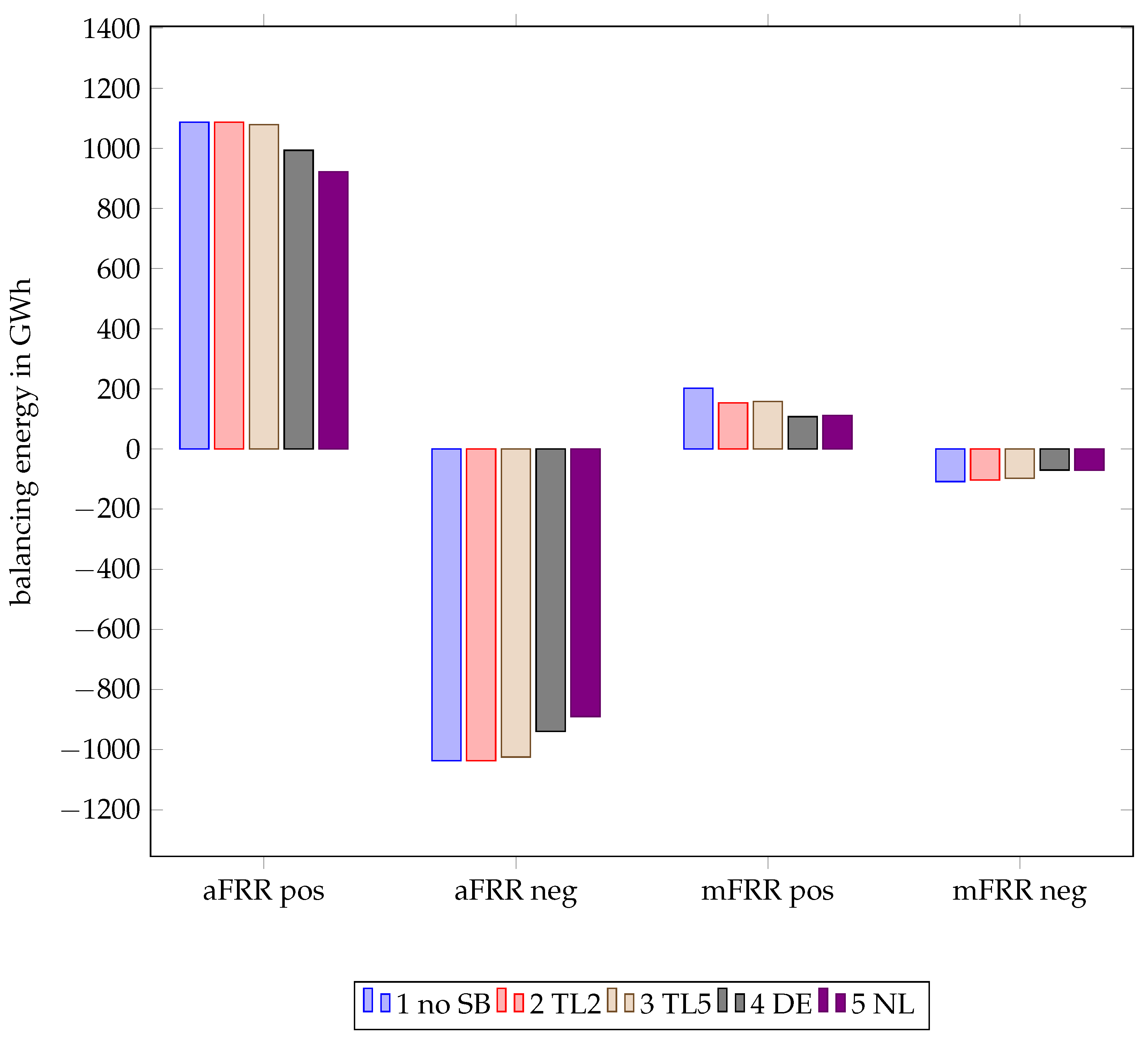
Figure 6 illustrates the absolute demand for positive and negative aFRR and mFRR over the simulated year 2019. All scenarios supported the hypothesis that smart balancing reduced the ACE and demand for balancing energy. The results showed that the traffic light approaches mainly reduced the mFRR demand, while aFRR could only be reduced in scenarios with full transparency.

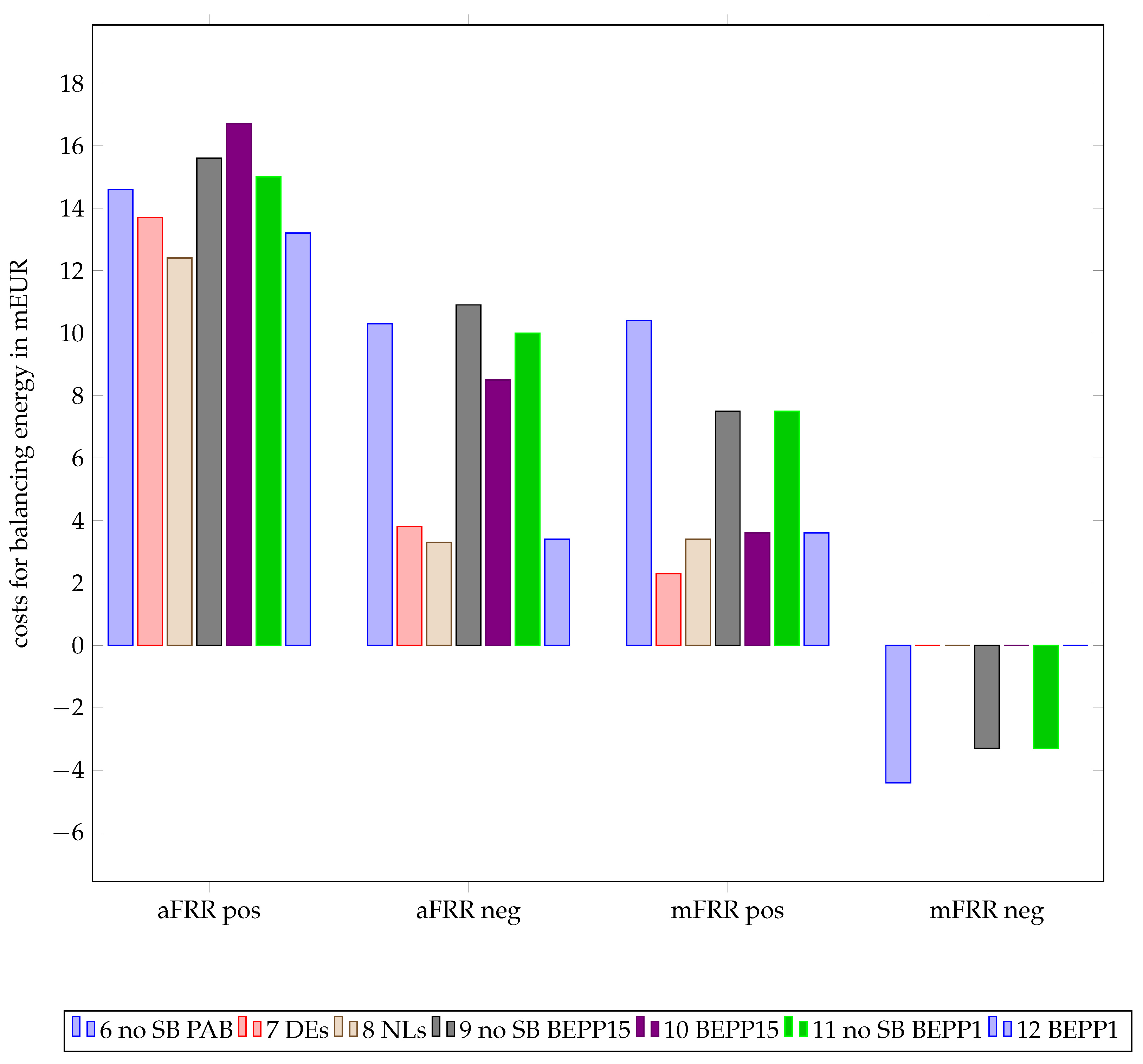
Figure 7 illustrates the absolute costs for positive and negative aFRR and mFRR over the simulated year 2019. Negative costs represent profit from the system perspective. The costs for positive aFRR and positive mFRR were reduced with smart balancing. The profits from activating negative aFRR were increased with smart balancing, but the profit from activating negative mFRR was reduced.

Table 9. Smart balancing simulation: results of scenarios with historic ACE and pay-as-bid clearing.

Scenario	f Mean	f std	f Min	f Max
1 No smart balancing	50 Hz	0.0108 Hz	49.843 Hz	50.135 Hz
2 Traffic light TL2	50 Hz	0.0116 Hz	49.631 Hz	50.287 Hz
3 Traffic light TL3	50 Hz	0.0111 Hz	49.641 Hz	50.199 Hz
4 Single pricing DE	50 Hz	0.0123 Hz	49.759 Hz	50.179 Hz
5 Combined pricing NL	50 Hz	0.0113 Hz	49.763 Hz	50.174 Hz

shows the simulated effect of smart balancing on the frequency of the Central-West European synchronous zone. In all cases, the frequency standard deviation (std) was higher, and outliers (min, max) had a bigger distance to the set value of 50 Hz in scenarios with smart balancing. Therefore, the results indicated that smart balancing could have a negative side effect on the quality of the frequency.

The reason for the decrease in frequency quality with reduced demand for FRR is illustrated in Figure 8. The figure showcases the worst imbalance event of the year 2019 with activated reserves of over 7 GW and simulation results of the traffic light scenarios TL2 and TL5. The ACE and the demand for FRR could be reduced during each ISP, but going back to schedule at the end of each ISP led to high-frequency deviations.

Figure 8 also illustrates the difference between the two traffic light scenarios TL2 and TL5 in the case of high imbalance events. There was no further differentiation in case of an ACE that was higher than 100% of the contracted FRR. TL6, on the other hand, changed the signal at 12:00 from ”over 150%“ to ”over 120%”, and a reduced smart balancing contribution was the result. The slightly higher smart balancing contribution with the TL2 approach before 12:00 can be traced back to the fuzzy logic, where less membership functions were defined in the TL2, scenario leading to a higher output for “good smart balancing”.

3.2. Simulation with Synthetic Data

As explained in Section 2.2.3 and Section 2.5, the historic ACE includes “under-cover” smart balancing and MOLs resulted from a pay-as-bid clearing environment. On order to exclude these effects from the simulation, synthetic data instead of the historic data were used for the following simulations. Section 2.2.4 introduces the applied synthetic data.

Table 10. Smart balancing simulation-activated FRR energy and total costs of scenarios with synthetic ACE.

Scenario	pos. aFRR	neg. aFRR	pos. mFRR	neg. mFRR	Total Costs
6 no smart balancing PAB	100%	100%	100%	100%	100%
7 DEs	95%	66%	27%	0%	64%
8 NLs	91%	59%	39%	0%	62%
9 no SB BEPP15	98%	94%	74%	75%	99%
10 BEPP: 15 min	92%	55%	39%	0%	93%
11 no SB BEPP1	98%	94%	74%	75%	94%
12 BEPP: 1 min	91%	56%	39%	0%	65%

shows the reduction of balancing energy and related costs relative to the simulation without smart balancing and pay-as-bid clearing. As explained in Section 2.2.4, the MOLs for marginal clearing were chosen to result in similar costs with a 15-min BEPP, but no further differentiation of the MOLs was applied for the 1-min BEPP. As expected, this led to a decrease of the total costs compared to pay-as-bid or marginal clearing with a 15-min BEPP.

Again, the demand for FRR and the total costs for balancing energy were reduced with all smart balancing concepts. The activation of negative mFRR could even be reduced to zero by smart balancing. This could be achieved by a negative flexibility potential of DSI and renewable energies, as introduced in Section 2.3.1. Combined pricing “8 NLs” outperformed the approach with pure single pricing “7 DEs”. In comparison to the simulation with historic data, this effect was less distinct. Nevertheless, the results further supported the hypothesis that combined pricing improves the smart balancing contribution.

The effect of the imbalance pricing scheme outweighed the influence of the clearing scheme on efficiency of the smart balancing approach. The three scenarios “8 NLs”, “10 BEPP: 15 min”, and “12 BEPP: 1 min” were all simulated with combined pricing, but different FRR clearing schemes. Figure 9 illustrates that the differences in the activated FRR of the three scenarios were very small.

In contrast to the demand of FRR, the related costs did differ, not only with the imbalance pricing, but also with the clearing scheme. Figure 10 illustrates that smart balancing could reduce the total costs only by 6% with marginal clearing and a 15-min BEPP, but the cost reduction accounted for 35% with marginal clearing and a 1-min BEPP.

Table 11. Smart balancing simulation: results of scenarios with historic ACE and pay-as-bid clearing.

Scenario	f Mean	f std	f Min	f Max
6 no smart balancing PAB	50 Hz	0.0025 Hz	49.976 Hz	50.013 Hz
7 single pricing DE	50 Hz	0.0097 Hz	49.951 Hz	50.061 Hz
8 combined pricing NL	50 Hz	0.0085 Hz	49.931 Hz	50.063 Hz
9 no smart balancing BEPP15	50 Hz	0.0024 Hz	49.979 Hz	50.012 Hz
10 BEPP15	50 Hz	0.0116 Hz	49.901 Hz	50.071 Hz
11 no smart balancing BEPP1	50 Hz	0.0024 Hz	49.979 Hz	50.012 Hz
12 BEPP1	50 Hz	0.0093 Hz	49.932 Hz	50.073 Hz

shows the effect of smart balancing on the system frequency. The difference between the scenario “6 no smart balancing pay-as-bid” with higher frequency deviation in comparison to the two scenarios “9 no smart balancing BEPP15” and “11 no smart balancing BEPP1” resulted from the different ACE, as introduced in Section 2.2.4. Similar to the simulations with historic data, the simulations with synthetic data also indicated that smart balancing could have a negative effect on the frequency quality. Again, this can be traced back to the behavior at the end of an ISP when BRPs return to their schedule (see Figure 5).

3.3. Results from the Perspective of Participating Technologies

We compared the different scenarios from a participant technology perspective by energy, profit, specific energy purchase costs, number of balancing participation, and their average duration. Energy and profit data were used to specify the participation profile. Is more energy consumed or produced? Did a technology manage to generate profit from the participation in smart balancing, or was money lost? This information was used to assess the suitability of the different approaches for the single technologies. To give a more detailed assessment of the balancing behavior, the number of balancing actions was counted, and the average duration of the balancing action was calculated. In the case of a very short duration, it might be necessary to do further investigations on the impact of rapid load changes on the plants’ operation and lifetime. The comparison of total profits and energy included the installed capacity and balancing potential of the single technologies. For a comparison of the monetary benefit for the participating technologies, therefore, the specific energy purchase costs were analyzed.

3.3.1. Technologies

In a first step, the single technologies’ total energy balance and their overall profit were investigated. The energy balances are visualized in

Table 12. Overview of the technologies’ energy balance in the investigated scenarios.

Scenario	Sol	WOn	WOf	Gas	Alu	Ste	Cem	Pap	Chl
Historic data
2 TL2	- - -	- - -	- - -	+	++	+++	+	+	+
3 TL5	- - -	- - -	- - -	+	++	+++	+	+	+
4 DE	- -	- -	- - -	+++	+++	0	- - -	- - -	- - -
5 NL	-	- -	- - -	+++	++	0	- - -	- - -	- - -
Synthetic data
7 DEs	-	-	-	+++	++	0	- - -	- - -	- - -
8 NLs	–	-	- -	++	+++	0	- - -	- - -	- - -
10 BEPP: 15 min	- - -	- - -	- - -	-	+++	0	- - -	- - -	- - -
12 BEPP: 1 min	- -	- -	- -	+	+++	0	- - -	- - -	- - -

, and related profits can be read from

Table 13. Overview of the technologies’ profit in the investigated scenarios.

Scenario	Sol	WOn	WOf	Gas	Alu	Ste	Cem	Pap	Chl
Historic data
2 TL2	- - -	- - -	- - -	+	+++	+++	+++	+++	+++
3 TL5	- - -	- - -	- - -	+	++	+++	+++	+++	+++
4 DE	- - -	- - -	- - -	+++	+++	0	-	++	–
5 NL	+++	+++	+++	+++	++	0	++	+++	++
Synthetic data
7 DEs	+	+	+	+++	+	0	++	++	++
8 NLs	+	+	+	+++	++	0	++	++	++
10 BEPP: 15 min	+++	+++	+++	+++	+++	0	+++	+++	+++
12 BEPP: 1 min	++	++	++	+++	++	0	++	++	++

. To enable a good overview about all technologies and scenarios, the values for energies and profits were simplified and clustered as described in

Table 14. Legend for Table 12 and Table 13.

Energy
+	increase production = decrease consumption
-	decrease production = increase consumption
Profit
+	profits
-	losses
Ranges
+++/- - -	x > 2/3 of technologies maximum/minimum value
++/- -	1/3 < x < 2/3 of technologies maximum/minimum value
+/-	1/20 < x < 1/3 of technologies maximum/minimum value
0	x < 1/20 of technologies maximum/minimum value

.

Solar power plants achieved monetary benefits by reducing their feed-in in more than half of the scenarios. Exceptions were TL2, TL5, and the DE approach based on historic data. The same applied for wind onshore and wind offshore.

Aluminum and steel gained profits by reducing their demand. This applied for all scenarios including the exception that steel did not participate in the scenarios based on synthetic data. The revenues from demand reduction varied between 61 and 143 EUR/MWh for aluminum and from 105 and 234 EUR/MWh for steel.

In the TL2 and TL5 scenarios, cement, paper, and chlorine also reduced their demand for revenues between 108 and 127 EUR/MWh. In the other scenarios, the three technologies increased their demands and achieved profits that way. In the case of the DE approach, cement and chlorine had additional costs of 0.8 and 4.1 EUR/MWh for increasing their demand. In the other scenarios, profits from 5 to 127 EUR/MWh were made.

Gas power plants mainly increased their production. There was only the BEPP 15-min scenario where production was decreased. Profit was generated in all cases. The revenues from lowering the production varied between 81 and 1373 EUR/MWh.

In scenarios based on synthetic data, the contribution of renewables and metal industries were generally less than those of the remaining industries and the gas power plants. In the NL scenario based on historic data, average values of below two minutes were observed for renewables, which was very short. The TL2 and TL5 approaches generally led to durations above 8 min for all technologies.

3.3.2. Overall Comparison

To be able to compare the benefit of the different scenarios for the single technologies, the specific costs or profits of the technologies smart balancing contributions were regarded. Therefore, it was distinguished whether there was an additional energy purchase or an increased production. A successful additional purchase might lead to costs lower than the average energy purchase costs. This is of importance for consumers like the industrial plants. In the case of renewable energy plants, changes in generation were successful only if profits were achieved by that, since there were no production costs to be saved. In the case of the gas power plants, both cases were possible.

Table 15. Overview of the technologies’ specific profits in the investigated scenarios.

Scenario	Sol	WOn	WOf	Gas	Alu	Ste	Cem	Pap	Chl
Historic data
2 TL2	(-)	(- -)	(-)	+	+++	++	+++	+++	+++
3 TL5	(- - -)	(- - -)	(- - -)	+	+++	++	+++	+++	+++
4 DE	(- -)	(- - -)	(- -)	+	+++	+++	-	+	-
5 NL	+	+	+	+	+++	+++	+	+	+
Synthetic data
7 DEs	++	+++	+++	+	++	none	+	+	+
8 NLs	++	++	++	++	++	none	+	+	+
10 BEPP: 15 min	+++	+++	+++	+++	+++	none	++	++	++
12 BEPP: 1 min	++	++	++	+++	++	none	+	+	+

gives an overview of the technologies’ specific profits in the different scenarios. As a reference, always the maximum profit from the regarded technology was chosen. The values for specific profits were simplified and clustered, as described in

Table 16. Legend for the table.

Specific Profit
+	profits
-	costs for energy purchase
(-)	costs from energy sales = losses
none	no values
Specific profits
+++	x > 2/3 of technologies maximum profit
++	1/3 < x < 2/3 of technologies maximum profit
+	1/20 < x < 1/3 of technologies maximum/profit
Specific energy purchase costs
-	x > 1/3 of technologies maximum profit
- -	1/3 < x < 2/3 of technologies maximum profit
- - -	2/3 < x < 1 of technologies maximum profit

.

From Table 15, it can be seen that the specific profits were more consistent in the synthetic data-based scenarios. The TL scenarios offered high profits for industries, but also losses for renewables. In the historic data scenarios, only the NL approach led to profits for all technologies. The highest specific profits were observed in the BEPP 15-min scenario, but also, the BEPP 1-min scenario had high specific profits. A comparison with the total profits confirmed the NL scenario and the BEPP 15-min scenario as the most profitable scenarios for all technologies.

3.3.3. Summary/Conclusions Technologies

From the evaluation of the single technologies’ data, it can be seen that the consistency between the data of different technologies was higher in scenarios based on synthetic data than in the scenarios based on historic data. Based on synthetic data, the highest revenues could be achieved in the BEPP 15-min scenario.

4. Discussion

Based on the model presented in Section 2, the simulation outcomes showed the effects different smart balancing schemes could have if applied in Germany. The impacts of the imbalance pricing (single vs. combined) and the method of balancing energy clearing (pay-as-bid vs. marginal pricing with 15-min BEPP vs. marginal pricing with 1-min BEPP) were quantified. The results supported the initial hypothesis that smart balancing can reduce the ACE closed loop and the demand for balancing energy activated via FRR products. In all considered scenarios, the demand for balancing energy and related costs were reduced by active smart balancing.

As expected, especially the reduction of manual FRR balancing energy was a direct consequence of smart balancing, since large system imbalances sustained for several ISPs were especially suitable for BRPs to support the system without taking high risks that the direction of the system imbalance changes and the imbalance price results in costs rather than revenues.

Regarding the FRR settlement, results were surprisingly similar when comparing pay-as-bid and marginal pricing in all the settings with each other. The potential of smart balancing was apparently not mainly driven by marginal pricing with a BEPP of 15 min. Nonetheless, a disclaimer has to be made for the applied pay-as-bid and marginal bidding curves with the synthetic data in our simulations. In cases where prices of balancing energy bids are more volatile and extreme, smart balancing would probably lead to better results in a marginal pricing scheme rather than in a pay-as-bid scheme.

The results were more driven by the technology chosen to contribute to smart balancing, especially since the demand-side integration technologies mainly provided downward energy in the simulations. For an application of smart balancing in Germany, the obtained real effects will obviously deviate from the presented effects.

For a gradual implementation of smart balancing in Germany, the traffic light concept might be a concept to be considered. Independent of the chosen layout of the German imbalance price calculation based on a PICASSO cycle-based BEPP, such a concept could support Germany during system scarcity and persistent imbalances exposed to the system.

Secondly, it is recommended to apply a combined pricing for imbalance in case the German system is exposed to zero-crossings.

Future research may focus on how active smart balancing could work best within the emerging European platforms IGCC and PICASSO. The damping effect of changing the BEPP in a future marginal clearing environment, including effects on the MOL, should be analyzed with higher accuracy. Regarding the applied fuzzy logic, further investigations on the effects of tuning fuzzy sets, fuzzy rules, type of inference, defuzzification technique, and type-1 vs. type-2 fuzzy logic can improve the understanding of market response. Other smart balancing algorithms could also lead to similar results, and future work could investigate the effect of replacing the fuzzy logic by conventional decision trees or applying machine learning. On the other hand, simulation-based research cannot predict the real market behavior without big uncertainties, as described in Section 2.4. This limitation leads to the need for field tests to generate more profound knowledge about active smart balancing and its value.

5. Conclusions

The simulation with synthetic ACE and MOL confirmed the findings from the pay-as-bid simulations with historic data. Combined pricing is more beneficial than single pricing. The scenarios with combined pricing and marginal clearing could benefit from smart balancing and reduce the demand for balancing reserves in a similar range, but related costs substantially decreased only in the case of a 1-min BEPP. This could be traced back to the limited reflection of bidding behavior, as no difference between the two marginal pricing scenarios (BEPP15 vs. BEPP1) was assumed. Nevertheless, the result that smart balancing saved a higher share of the total costs with pay-as-bid pricing confirmed the correlation between cost and imbalance occurrence, illustrated in Figure 3. The results were considered to be plausible, because BRPs would have generated profit with their behavior.

Other findings could be made from defining the smart balancing decision making process of BRPs in the first place. Implementing a fuzzy logic which leads to profit for BRPs is required to limit the reaction in order to prevent overreaction and financial losses, as described in Section 2 and Appendix A. Nevertheless, the introduction of active smart balancing could lead to overreaction and financial losses on the first day. An optimization of smart balancing, similar to the tuning of fuzzy rules, might be seen in real operations. This hypothesis is supported by the observations made in The Netherlands in 2001, when the smart balancing was introduced and improved over time [9].

As a consequence, to reduce the risks from potential overreactions, a damping of smart balancing with the traffic light approach or a limitation of financial incentives could be chosen for a first introduction period. Pay-as-bid clearing and marginal clearing with a short BEPP would limit the incentive in comparison to marginal pricing with 15-min BEPP. On the other hand, the optimization of BRPs could make damping unnecessary.

In contrast to the reduction of demand and costs for balancing energy, the simulation indicates that smart balancing might have a negative effect on the overall frequency stability at the transition form one ISP to the next. The higher deviation and lower minimum and higher maximum of the frequency result from the fast reaction, especially at the end of each ISP, when all BRPs return to their schedule. Such an extreme behavior is not seen in real operations in The Netherlands and Belgium, but the smart balancing logic in the simulation led to this fast behavior in response to the uncertain source of the ACE, which also reflected scheduled energy exchanges with other control blocks and can, therefore, change in the beginning of an ISP.

References

- European Commission. Commission Regulation (eu) 2017/2195-of 23 November 2017-Establishing a Guideline on Electricity Balancing. Off. J. Eur. Union 2017. Available online: https://eur-lex.europa.eu/eli/reg/2017/2195/oj (accessed on 18 April 2021).
- Hirth, L.; Ziegenhagen, I. Balancing Power and Variable Renewables: Three Links. Renew. Sustain. Energy Rev. 2015, 50, 1035–1051. [Google Scholar] [CrossRef]
- Nobel, F. On Balancing Market Design. Ph.D. Thesis, Technische Universiteit Eindhoven, Eindhoven, The Netherlands, 2016. [Google Scholar]
- Brijs, T.; De Jonghe, C.; Hobbs, B.F.; Belmans, R. Interactions between the Design of Short-Term Electricity Markets in the CWE Region and Power System Flexibility. Appl. Energy 2017, 195, 36–51. [Google Scholar] [CrossRef]
- Tennet, H.B. Balance Delta with IGCC. 2019. Available online: https://www.tennet.org/english/operational_management/System_data_relating_implementation/system_balance_information/balancedeltaIGCC.aspx (accessed on 18 April 2021).
- Elia, T.B.S. Imbalance Prices. 2020. Available online: https://www.elia.be/en/grid-data/balancing/imbalance-prices-1-min (accessed on 18 April 2021).
- Federal Network Agency Germany, Bundesnetzagentur. BK6-06-013 Beschluss: Festlegung zur Vereinheitlichung der Bilanzkreisverträge. Available online: https://www.bundesnetzagentur.de/DE/Beschlusskammern/1_GZ/BK6-GZ/2006/BK6-06-013/BK6-06-013_Beschluss.html (accessed on 19 December 2017).
- Olmos, L.; Rodilla, P.; Fernandes, C.; Frias, P.; Fontaine, A.; Loureiro, R.; Caetano, B.; Dourlens, S.; Döring, T.; Wright, H.; et al. D3.2 Developments Affecting the Design of Short-Term Markets. 2015, p. 144. Available online: http://market4res.eu/wp-content/uploads/D3.2_20151009_final.pdf (accessed on 18 April 2021).
- Beune, R.J.L.; Nobel, F. System Balancing in The Netherlands. In Methods to Secure Peak Load Capacity on Deregulated Electricity Markets; Market Design: Saltsjöbaden, Sweden, 2001; pp. 47–58. [Google Scholar]
- Elia. End User Documentation—“1-Minute Publications” on Elia. Available online: https://www.elia.be/-/media/project/elia/elia-site/grid-data/balancing/20190827_end-user-documentation-elia1-minute-publications.pdf (accessed on 18 April 2021).
- ENTSO-E. Continental Europe Operational Handbook, “P1—Policy 1: Load-Frequency Control and Performance [C]” & “A1—Appendix 1: Load-Frequency Control and Performance [E]”. Available online: https://entsoe.eu/fileadmin/user_upload/_library/publications/entsoe/Operation_Handbook/Policy_1_final.pdf (accessed on 18 April 2021).
- Franz, J.; Röben, F. Market Response for Real-Time Energy Balancing—Simulation Using Field Test Data. In Proceedings of the 2020 17th International Conference on the European Energy Market (EEM), Stockholm, Sweden, 16–18 September 2020; pp. 1–5. [Google Scholar] [CrossRef]
- 50 Hertz; Amprion; TenneT; TransnetBW Ermittlung reBAP und Umgang Mit Korrekturen (Gültig Ab 01.07.2020).Pdf. Available online: https://www.regelleistung.net/ext/static/rebap (accessed on 18 April 2021).
- Röben, F.; Schäfers, H. Integration of Power Balancing Markets in Europe—Transparency as a Design Variable. In Proceedings of the 2018 41th IAEE Conference Transforming Energy Markets, Groningen, The Netherlands, 10–13 June 2018. [Google Scholar]
- Haghighat, H.; Seifi, H.; Kian, A.R. Pay-as-Bid versus Marginal Pricing: The Role of Suppliers Strategic Behavior. Int. J. Electr. Power Energy Syst. 2012, 42, 350–358. [Google Scholar] [CrossRef]
- Ocker, F.; Ehrhart, K.M. The “German Paradox” in the Balancing Power Markets. Renew. Sustain. Energy Rev. 2017, 67, 892–898. [Google Scholar] [CrossRef]
- Ocker, F.; Ehrhart, K.M.; Ott, M. Bidding Strategies in Austrian and German Balancing Power Auctions. Wiley Interdiscip. Rev. Energy Environ. 2018, 7, e303. [Google Scholar] [CrossRef]
- Belica, M.; Ehrhart, K.M.; Ocker, F. Harmonization of the European Balancing Power Auction: A Game-Theoretic and Empirical Investigation. Energy Econ. 2018, 73, 194–211. [Google Scholar]
- 50 Hertz; Amprion; TenneT; TransnetBW Internetplattform Zur Vergabe von Regelleistung. 2020. Available online: https://www.regelleistung.net/ (accessed on 18 April 2021).
- ENTSO-E. Stakeholder Document for the Principles of IGCC. Available online: https://www.entsoe.eu/network_codes/eb/imbalance-netting/ (accessed on 18 April 2021).
- Gruber, A.M. Zeitlich und Regional Aufgelöstes Industrielles Lastflexibilisierungspotenzial als Beitrag zur Integration Erneuerbarer Energien. Ph.D. Thesis, Technical University of Munich, Munich, Germany, 2017. [Google Scholar]
- Zadeh, L.A. Fuzzy Sets. Inf. Control 1965, 8, 338–353. [Google Scholar] [CrossRef]
- Mamdani, E. Application of Fuzzy Algorithms for Control of Simple Dynamic Plant. Proc. Inst. Electr. Eng. 1974, 121, 1585. [Google Scholar] [CrossRef]
- Warner, J.; Sexauer, J.; Scikit-Fuzzy, T.A.; Unnikrishnan, A.; Castelão, G.; Pontes, F.A.; Uelwer, T.; Batista, F.; Broeck, W.V.D.; Song, W.; et al. JDWarner/Scikit-Fuzzy: Scikit-Fuzzy Version 0.4.2. 2019. Available online: https://zenodo.org/record/3541386#.YH2K_j8RVPY (accessed on 18 April 2021).
- Röben, F.; Meißner, A. Market Response for Real-Time Energy Balancing with Fuzzy Logic. In Proceedings of the 2020 17th International Conference on the European Energy Market (EEM), Stockholm, Sweden, 16–18 September 2020; pp. 1–5. [Google Scholar] [CrossRef]
- ENTSO-E Central Collection and Publication of Electricity Generation, Transportation and Consumption Data. 2020. Available online: https://transparency.entsoe.eu/ (accessed on 18 April 2021).
- Eicke, A.; Ruhnau, O.; Hirth, L. Electricity Balancing as a Market Equilibrium: Estimating Supply and Demand of Imbalance Energy. 2020, p. 26. Available online: https://www.econstor.eu/handle/10419/223062 (accessed on 18 April 2021).
- Koch, C. Intraday Imbalance Optimization: Incentives and Impact of Strategic Intraday Bidding in Germany. SSRN Electron. J. 2019. [Google Scholar] [CrossRef]
- Röben, F.; de Haan, J.E.S. Market Response for Real-Time Energy Balancing—Evidence From Three Countries. In Proceedings of the 2019 16th International Conference on the European Energy Market (EEM), Ljubljana, Slovenia, 18–20 September 2019; pp. 1–5. [Google Scholar] [CrossRef]
Figure 1.
Smart balancing model: structure of objects and most important properties.
Figure 2.
Flowchart of smart balancing simulation.
Figure 3.
Correlation of costs and imbalance occurrence with pay-as-bid vs. marginal clearing of balancing energy.
Figure 4.
Example with marginal clearing of balancing energy: BEPP 15 min vs. BEPP 5 min.
Figure 5.
Details of smart balancing calculation in the simulation.
Figure 6.
Smart balancing simulation: demand of balancing energy in 2019.
Figure 7.
Smart balancing simulation: costs for balancing energy in 2019.
Figure 8.
Historic imbalance event 12.06.2019 (Hist), traffic light scenarios (TL2 vs. TL5), and contracted automatic and manual Frequency Restoration Reserves (FRR).
Figure 9.
Smart balancing simulation: demand of balancing energy in synthetic scenarios.
Figure 10.