
Hourly Variation of Wind Speeds in the Philippines and Its Potential Impact on the Stability of the Power System


Abstract
1. Introduction
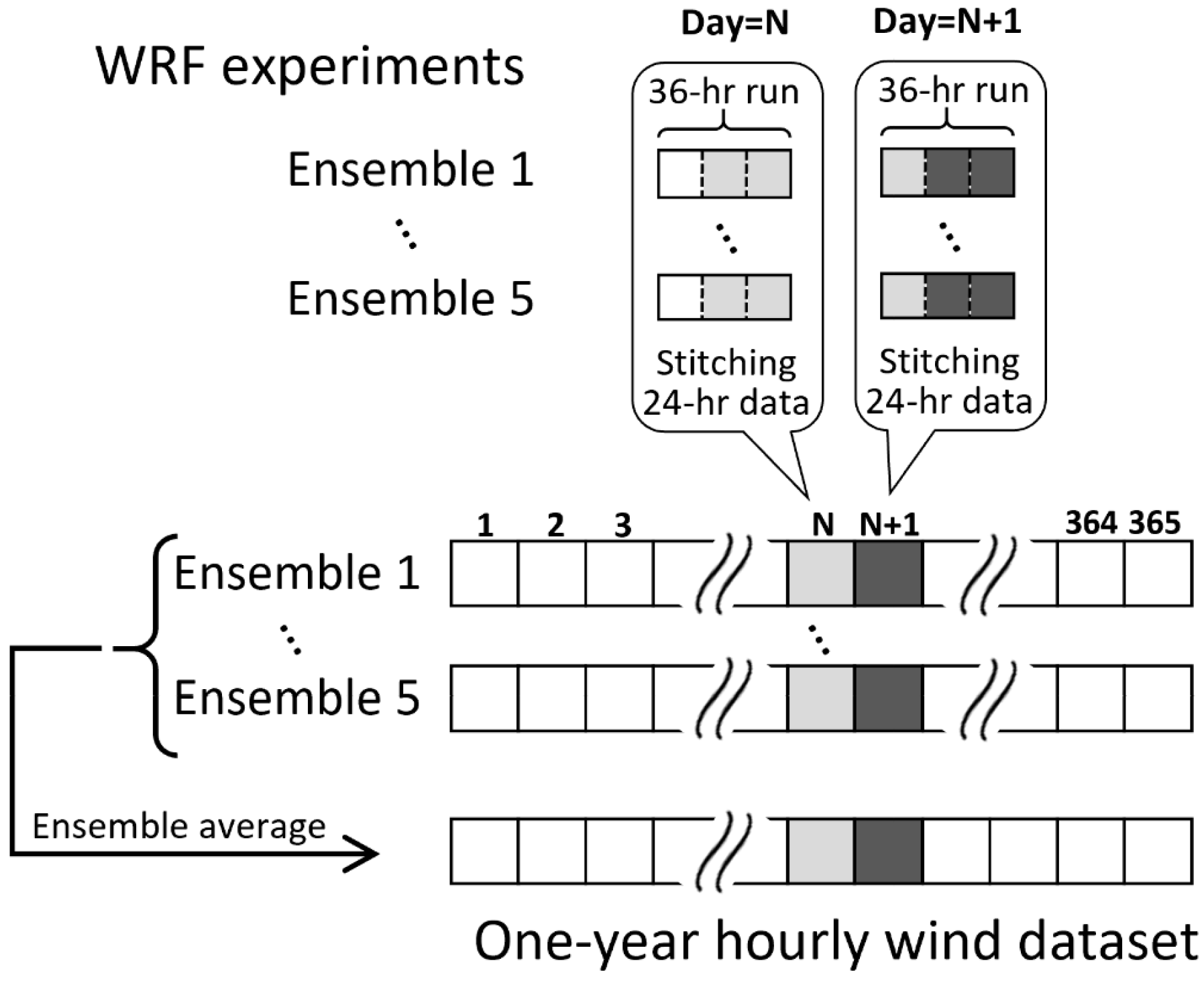
2. Methodology
3. Results and Discussions
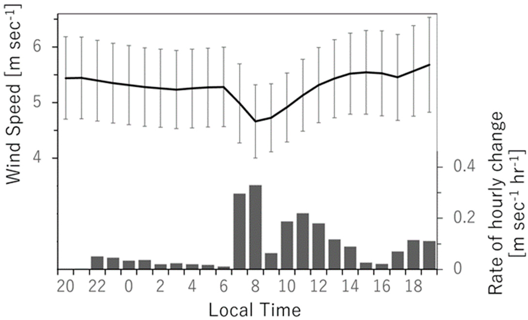
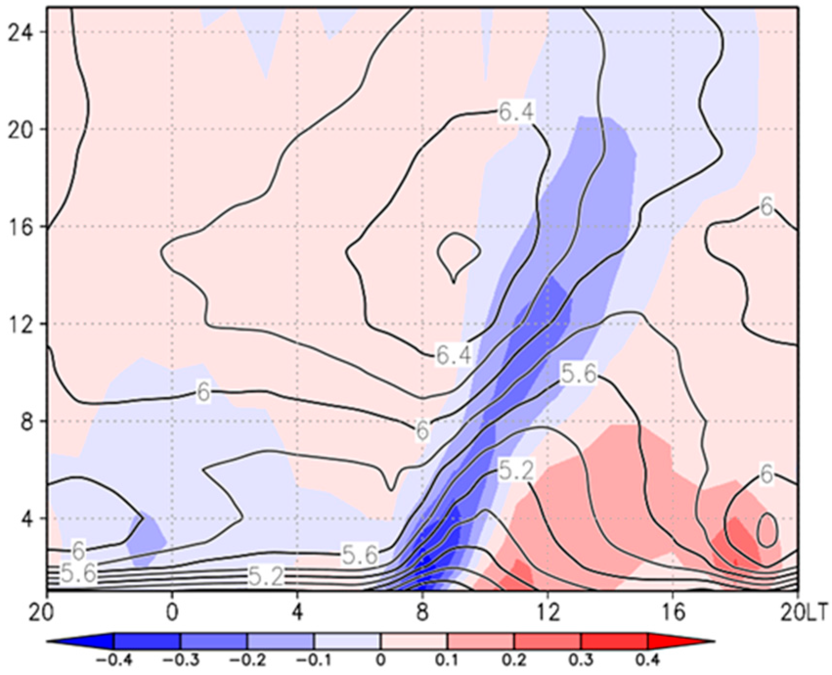
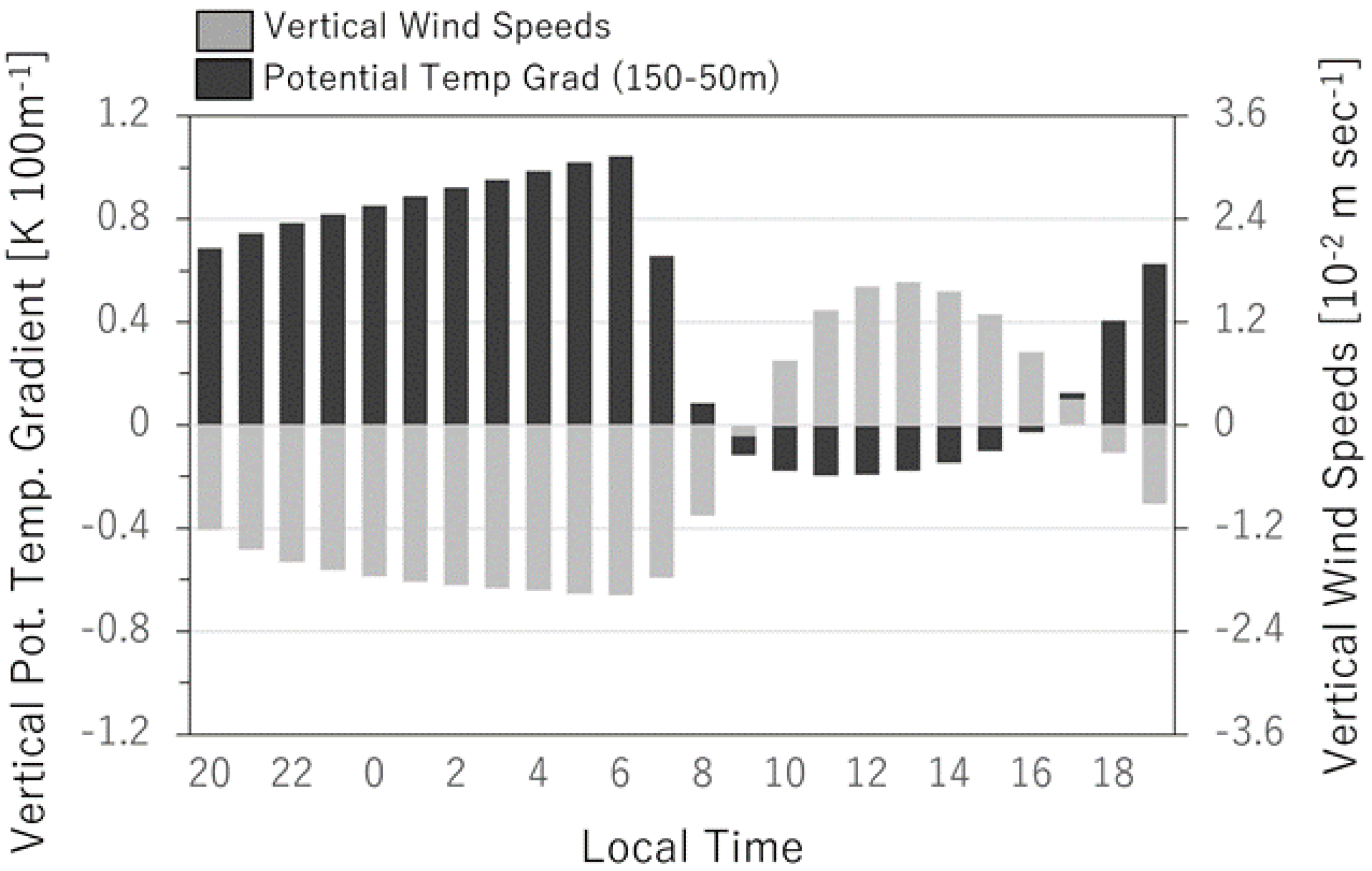
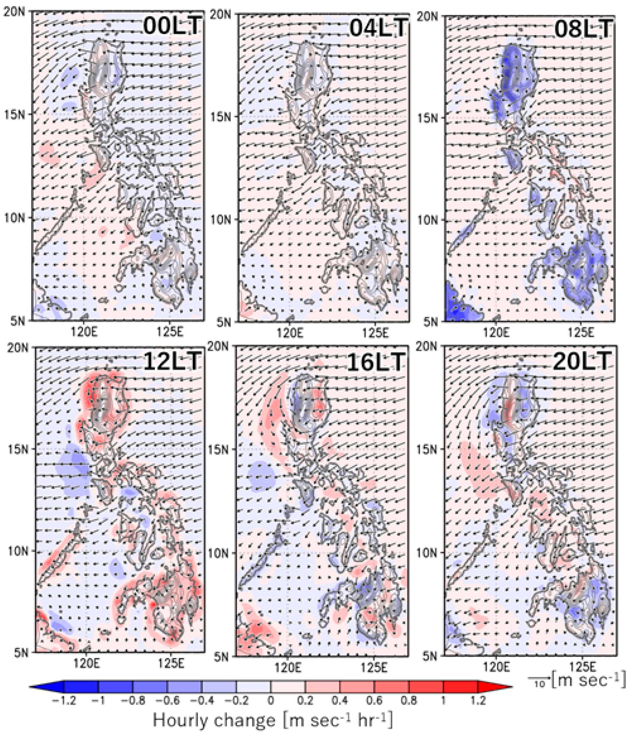
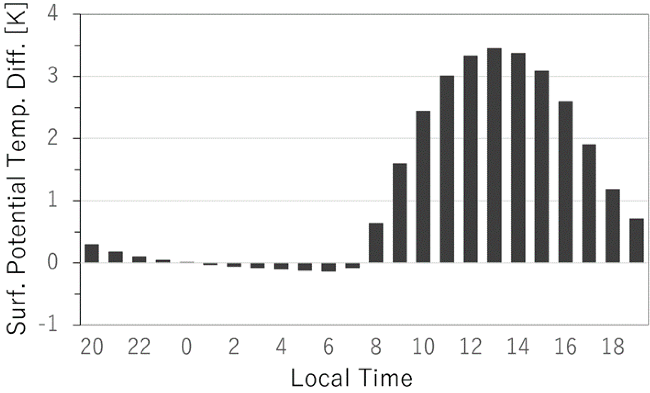
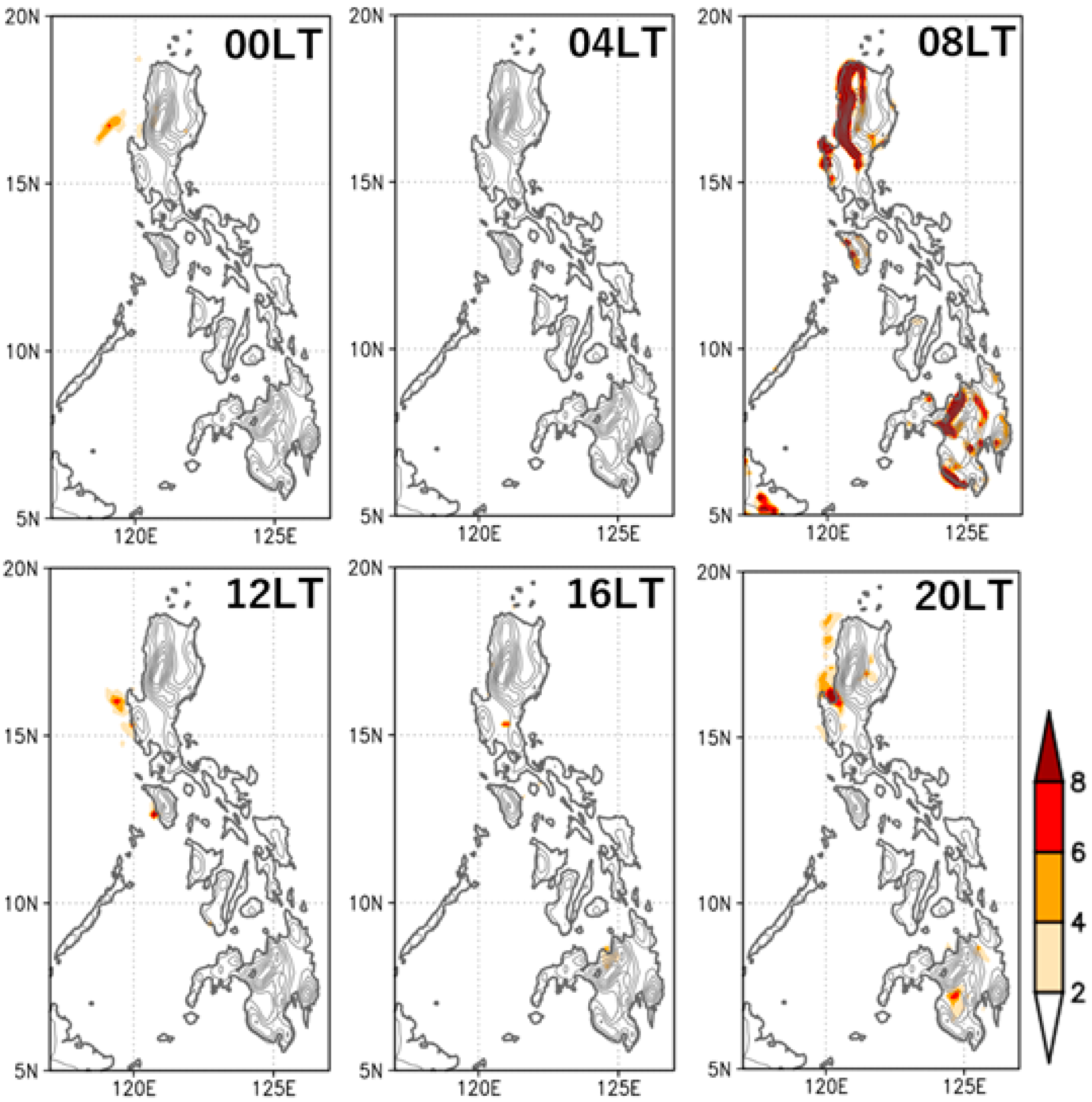
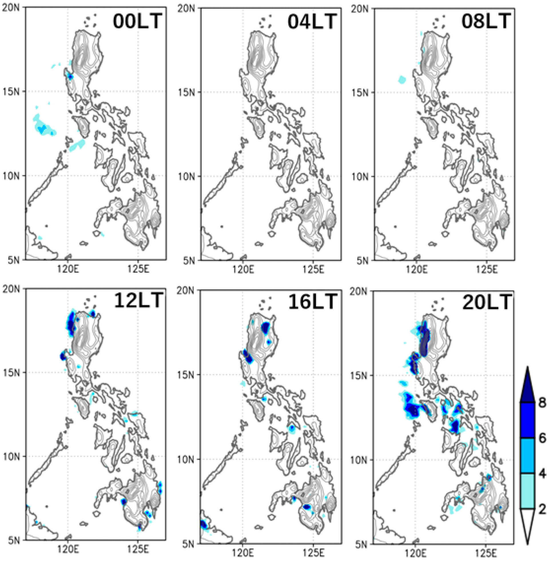
3.1. Hourly Variability in the Philippines within a Day
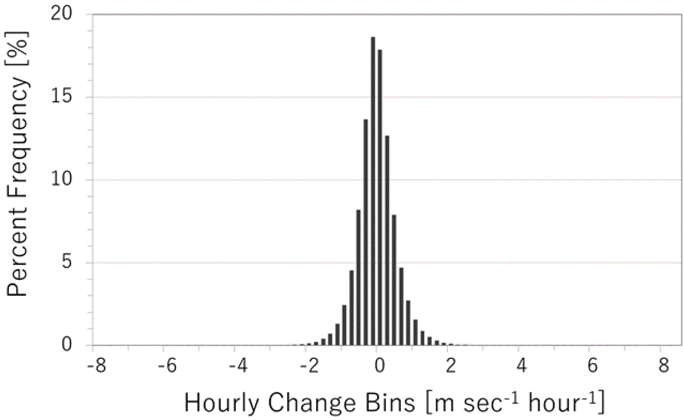
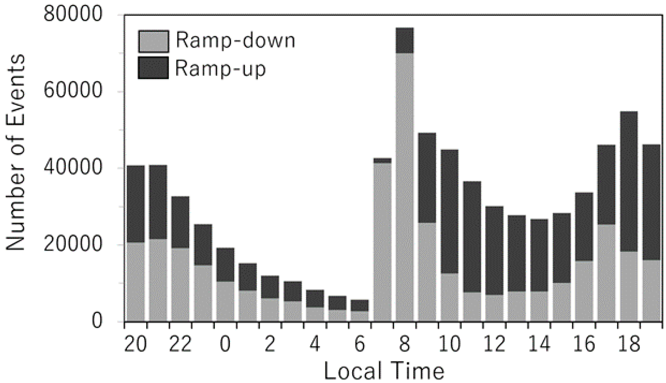
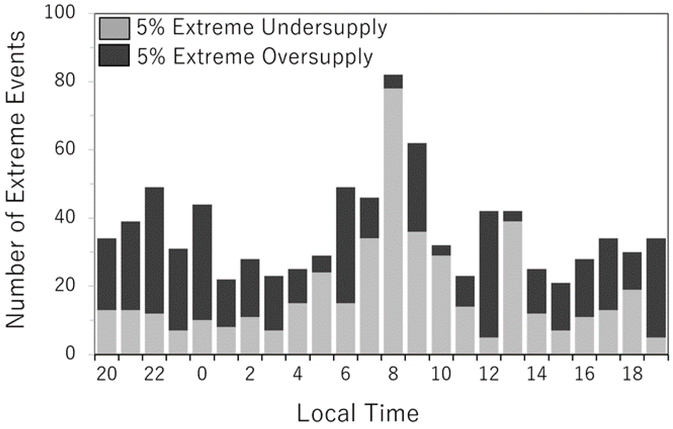
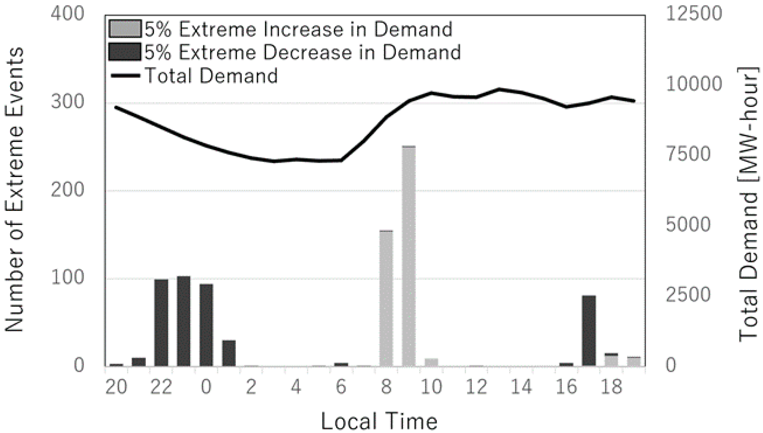
3.2. The Hourly Relationship between the Extreme Wind Variability and the Stability of the Power System
4. Conclusions
Author Contributions
Funding
Acknowledgments
Conflicts of Interest
References
- Engeland, K.; Borga, M.; Creutin, J.D.; François, B.; Ramos, M.H.; Vidal, J.P. Space-time variability of climate variables and intermittent renewable electricity production—A review. Renew. Sustain. Energy Rev. 2017. [Google Scholar] [CrossRef]
- Archer, C.L.; Colle, B.A.; Delle Monache, L.; Dvorak, M.J.; Lundquist, J.; Bailey, B.H.; Beaucage, P.; Churchfield, M.J.; Fitch, A.C.; Kosovic, B.; et al. Meteorology for coastal/offshore wind energy in the United States: Recommendations and research needs for the next 10 years. Bull. Am. Meteorol. Soc. 2014, 95, 515–519. [Google Scholar] [CrossRef]
- Elliott, D. Philippines Wind Energy Resource Atlas Development. In Business and Investment Forum for Renewable Energy and Energy Efficiency in Asia and the Pacific Region; National Renewable Energy Laboratory: Golden, CO, USA, 2000; pp. 1–10. [Google Scholar]
- NREL; USAID. Greening the grid: Solar and wind grid integration study for the Luzon-Visayas system of the Philippines. Altern. J. 2018, 27, 30–35. [Google Scholar]
- Marquis, M.; Wilczak, J.; Ahlstrom, M.; Sharp, J.; Stern, A.; Smith, J.C.; Calvert, S. Forecasting the wind to reach significant penetration levels of wind energy. Bull. Am. Meteorol. Soc. 2011, 92, 1159–1171. [Google Scholar] [CrossRef]
- Cutler, N.J.; Outhred, H.R.; MacGill, I.F.; Kepert, J.D. Predicting and presenting plausible future scenarios of wind power production from numerical weather prediction systems: A qualitative ex ante evaluation for decision making. Wind Energy 2012, 15, 473–488. [Google Scholar] [CrossRef]
- Klink, K. Atmospheric circulation effects on wind speed variability at turbine height. J. Appl. Meteorol. Climatol. 2007, 46, 445–456. [Google Scholar] [CrossRef]
- Deppe, A.J.; Gallus, W.A.; Takle, E.S. A WRF ensemble for improved wind speed forecasts at turbine height. Weather Forecast. 2013, 28, 212–228. [Google Scholar] [CrossRef]
- Drew, D.R.; Cannon, D.J.; Brayshaw, D.J.; Barlow, J.F.; Coker, P.J. The impact of future offshore wind farms on wind power generation in Great Britain. Resources 2015, 4, 155–171. [Google Scholar] [CrossRef]
- Cannon, D.J.; Brayshaw, D.J.; Methven, J.; Coker, P.J.; Lenaghan, D. Using reanalysis data to quantify extreme wind power generation statistics: A 33 year case study in Great Britain. Renew. Energy 2015, 75, 767–778. [Google Scholar] [CrossRef]
- Wallace, J.M.; Hobbs, P.V. Atmospheric Science: An Introductory Survey, 2nd ed.; Academic Press: Amsterdam, The Netherlands, 2006. [Google Scholar] [CrossRef]
- Hancock, P.E.; Zhang, S. A wind-tunnel simulation of the wake of a large wind turbine in a weakly unstable boundary layer. Bound. Layer Meteorol. 2015, 156, 395–413. [Google Scholar] [CrossRef]
- Pena, A.; Rethore, P.-E.; Rathmann, O. Modeling large offshore wind farms under different atmospheric stability regimes with the Park wake model. Renew. Energy 2014, 70, 164–171. [Google Scholar] [CrossRef]
- He, Y.; Monahan, A.H.; McFarlane, N.A. Diurnal variations of land surface wind speed probability distributions under clear-sky and low-cloud conditions. Geophys. Res. Lett. 2013, 40, 3308–3314. [Google Scholar] [CrossRef]
- Sato, T.; Miura, H.; Satoh, M.; Takayabu, Y.N.; Wang, Y. Diurnal cycle of precipitation in the tropics simulated in a global cloud-resolving model. J. Clim. 2009, 22, 4809–4826. [Google Scholar] [CrossRef]
- Skamarock, W.C.; Klemp, J.B.; Dudhia, J.; Gill, D.O.; Liu, Z.; Berner, J.; Wang, W.; Powers, J.G.; Duda, M.G.; Barker, D.M.; et al. A Description of the Advanced Research WRF Version 4; NCAR Tech. Note NCAR/TN-556+STR; National Center for Atmospheric Research: Boulder, CO, USA, 2019. [Google Scholar] [CrossRef]
- Carvalho, D.; Rocha, A.; Gómez-Gesteira, M.; Silva Santos, C. Sensitivity of the WRF model wind simulation and wind energy production estimates to planetary boundary layer parameterizations for onshore and offshore areas in the Iberian Peninsula. Appl. Energy 2014, 135, 234–246. [Google Scholar] [CrossRef]
- Fernández-González, S.; Martín, M.L.; García-Ortega, E.; Merino, A.; Lorenzana, J.; Sánchez, J.L.; Rodrigo, J.S.; Sanchez, J.; Valero, F. Sensitivity analysis of the WRF model: Wind-resource assessment for complex terrain. J. Appl. Meteorol. Clim. 2018, 57, 733–753. [Google Scholar] [CrossRef]
- Smith, E.N.; Gibbs, J.A.; Fedorovich, E.; Klein, P.M. WRF model study of the Great Plains low-level jet: Effects of grid spacing and boundary layer parameterization. J. Appl. Meteorol. Clim. 2018, 57, 2375–2397. [Google Scholar] [CrossRef]
- Stull, R.B. An Introduction to Boundary Layer Meteorology; Springer: Dordrecht, The Netherlands, 1988. [Google Scholar] [CrossRef]
- Siebesma, A.P.; Soares, P.M.M.; Teixeira, J. A combined eddy-diffusivity mass-flux approach for the convective boundary layer. J. Atmos. Sci. 2007, 64, 1230–1248. [Google Scholar] [CrossRef]
- Dee, D.P.; Uppala, S.M.; Simmons, A.J.; Berrisford, P.; Poli, P.; Kobayashi, S.; Andrae, U.; Balmaseda, M.A.; Balsamo, G.; Bauer, D.P.; et al. The ERA-Interim reanalysis: Configuration and performance of the data assimilation system. Q. J. R. Meteorol. Soc. 2011, 137, 553–597. [Google Scholar] [CrossRef]
- Dee, D.P.; Balmaseda, M.; Balsamo, G.; Engelen, R.; Simmons, A.J.; Thépaut, J.N. Toward a consistent reanalysis of the climate system. Bull. Am. Meteorol. Soc. 2014, 95, 1235–1248. [Google Scholar] [CrossRef]
- University Corporation for Atmospheric Research (UCAR). NAMELIST.INPUT: Best Practices. WRF Users Page. Available online: https://www2.mmm.ucar.edu/wrf/users/namelist_best_prac_wrf.html (accessed on 18 April 2021).
- Ulmer, F.-G.; Balss, U. Spin-up time research on the weather research and forecasting model for atmospheric delay mitigations of electromagnetic waves. J. Appl. Remote Sens. 2016, 10, 16027. [Google Scholar] [CrossRef]
- FirstGen; Philippine Electric Market Corporation (PEMC). Philippine Power System Data: Hourly System Demand, Dispatched Energy, and System Frequency for 2017; PEMC: Manila, Philippines, 2019. [Google Scholar]
- Kimura, F.; Kuwagata, T. Horizontal heat fluxes over complex terrain computed using a simple mixed-layer model and a numerical model. J. Appl. Meteorol. Climatol. 1995, 34, 549–558. [Google Scholar] [CrossRef][Green Version]
- Gierach, M.M.; Graber, H.C.; Caruso, M.J. SAR-derived gap jet characteristics in the lee of the Philippine Archipelago. Remote Sens. Environ. 2012, 117, 289–300. [Google Scholar] [CrossRef]
- Ohba, M.; Nohara, D.; Kadokura, S. Impacts of synoptic circulation patterns on wind power ramp events in East Japan. Renew. Energy 2016, 96, 591–602. [Google Scholar] [CrossRef]
- Martínez-Lucas, G.; Sarasúa, J.I.; Sánchez-Fernández, J.A. Frequency regulation of a hybridwind-hydro power plant in an isolated power system. Energies 2018, 11, 239. [Google Scholar] [CrossRef]
- Mondal, M.A.H.; Rosegrant, M.; Ringler, C.; Pradesha, A.; Valmonte-Santos, R. The Philippines energy future and low-carbon development strategies. Energy 2018, 147, 142–154. [Google Scholar] [CrossRef]
- IRENA. Future of Wind: Deployment, Investment, Technology, Grid Integration and Socio-Economic Aspects (A Global Energy Transformation Paper). 2019. Available online: https://www.irena.org/-/media/Files/IRENA/Agency/Publication/2019/Oct/IRENA_Future_of_wind_2019.pdf (accessed on 18 April 2021).


| Category | Name | Description | WRF’s Namelist Settings |
|---|---|---|---|
| Combination of Surface Layer (SL) and Planetary Boundary Layer (PBL) parameterization schemes | MM5YSU | MM5 SL similarity scheme combined with the Yonsei University (YSU) PBL scheme | sf_sfclay_physics = 1 bl_pbl_physics = 1 |
| ETAMYJ | ETA SL similarity scheme combined with the Mellor–Yamada–Janic (MYJ) PBL scheme | sf_sfclay_physics = 2 bl_pbl_physics = 2 | |
| PXACM2 | Pleim-Xiu (PX) SL scheme combined with the Asymmetric Convective Model Version 2 (ACM2) PBL scheme | sf_sfclay_physics = 7 bl_pbl_physics = 7 | |
| QNQNSE | Quasi-Normal Scale Elimination (QNSE) SL scheme combined with the QNSE PBL scheme | sf_sfclay_physics = 4 bl_pbl_physics = 4 | |
| MYNN25 | Mellor–Yamada Nakanishi and Niino (MYNN) SL scheme combined with the MYNN level 2.5 (MYNN25) PBL scheme | sf_sfclay_physics = 5 bl_pbl_physics = 5 |
Publisher’s Note: MDPI stays neutral with regard to jurisdictional claims in published maps and institutional affiliations. |
© 2021 by the authors. Licensee MDPI, Basel, Switzerland. This article is an open access article distributed under the terms and conditions of the Creative Commons Attribution (CC BY) license (https://creativecommons.org/licenses/by/4.0/).
Share and Cite
Lucas, K.R.E.; Sato, T.; Ohba, M. Hourly Variation of Wind Speeds in the Philippines and Its Potential Impact on the Stability of the Power System. Energies 2021, 14, 2310. https://doi.org/10.3390/en14082310
Lucas KRE, Sato T, Ohba M. Hourly Variation of Wind Speeds in the Philippines and Its Potential Impact on the Stability of the Power System. Energies. 2021; 14(8):2310. https://doi.org/10.3390/en14082310
Chicago/Turabian StyleLucas, Kevin Ray Español, Tomonori Sato, and Masamichi Ohba. 2021. "Hourly Variation of Wind Speeds in the Philippines and Its Potential Impact on the Stability of the Power System" Energies 14, no. 8: 2310. https://doi.org/10.3390/en14082310
APA StyleLucas, K. R. E., Sato, T., & Ohba, M. (2021). Hourly Variation of Wind Speeds in the Philippines and Its Potential Impact on the Stability of the Power System. Energies, 14(8), 2310. https://doi.org/10.3390/en14082310