Numerical Analysis of the Dynamic Interaction between Two Closely Spaced Vertical-Axis Wind Turbines

Abstract

To investigate the optimum layouts of small vertical-axis wind turbines, a two-dimensional analysis of dynamic fluid body interaction is performed via computational fluid dynamics for a rotor pair in various configurations. The rotational speed of each turbine rotor (diameter: D = 50 mm) varies based on the equation of motion. First, the dependence of rotor performance on the gap distance (gap) between two rotors is investigated. For parallel layouts, counter-down (CD) layouts with blades moving downwind in the gap region yield a higher mean power than counter-up (CU) layouts with blades moving upwind in the gap region. CD layouts with gap/D = 0.5–1.0 yield a maximum average power that is 23% higher than that of an isolated single rotor. Assuming isotropic bidirectional wind speed, co-rotating (CO) layouts with the same rotational direction are superior to the combination of CD and CU layouts regardless of the gap distance. For tandem layouts, the inverse-rotation (IR) configuration shows an earlier wake recovery than the CO configuration. For 16-wind-direction layouts, both the IR and CO configurations indicate similar power distribution at gap/D = 2.0. For the first time, this study demonstrates the phase synchronization of two rotors via numerical simulation.

1. Introduction

In a wind farm comprising numerous large-scale horizontal-axis wind turbines (HAWTs), the distance between adjacent turbine rotors must be several times longer than the rotor diameter. Otherwise, the power output will decrease significantly when a turbine is located in the wake of an upstream turbine. By predicting the wake of the turbines [1,2], the optimal layout of turbines that maximizes the wind farm power density (output per unit land area) can be identified—an important issue in the wind power field. Although vertical-axis wind turbines (VAWTs) do not prevail currently, as the basis for considering the optimal layout of the VAWT wind farm, Rajagopalan et al. conducted computational fluid dynamics (CFD) simulations assuming a two-dimensional (2D) laminar flow field [3]. Their results indicated that the rotors on the downwind side, but outside of the wake, produced a higher power output than the first-row rotors that faced the undisturbed flow owing to the interactions between the VAWT rotors. Meanwhile, Dabiri et al. proposed the possibility of closely spaced counter-rotating VAWT arrays, which can enhance the wind farm power density to a greater degree than existing HAWT wind farms; they conducted a numerical simulation based on a potential flow model incorporating velocity deficit [4] and field experiments using actual small VAWTs (Windspire: 1.2 kW) [5,6]. CFD analyses targeting a counter-rotating VAWT pair, which was used by Dabiri as a basis for the rotor array, have been recently conducted by many researchers. Zanforlin and Nishino performed 2D-CFD simulations of rotor models corresponding to Windspire and demonstrated that a counter-rotating closely spaced VAWT pair can produce a larger power output than an isolated single turbine [7]. Chen et al. conducted a 2D-CFD simulation targeting a straight-bladed VAWT pair and investigated the effects of five factors, i.e., inflow angle, tip speed ratio, turbine spacing, rotational direction, and blade angle, on the performance of a dual-turbine system [8]. Their results indicated that the power output of the rotor pair depended primarily on the tip speed ratio and inflow angle. De Tavernier et al. [9] comprehensively investigated the effects of rotor load (solidity), rotor spacing, and inflow angle on the flow and power output of a closely spaced 2D rotor pair (rotor radius = 10 m) via a 2D-CFD simulation based on a panel/vortex model. Ma et al. performed a 2D-CFD analysis to simulate a vertical-axis twin-rotor tidal current turbine, in which the two rotors revolved in opposite directions [10]. Based on the analysis, the maximum power coefficient was obtained at a tip speed ratio of 1.5, where the ratio of the rotor spacing to the diameter in the layout of the main flow perpendicular to the centerline connecting the two rotor centers was 9/4. As the rotor spacing became smaller than the optimal value, the power output decreased. As a special case corresponding to the ultimate close arrangement of the VAWT rotors, using three-dimensional (3D) CFD analysis, Poguluri et al. [11] investigated the 3D effects, such as the interaction of the tip vortices, of a co-axial contra-rotating VAWT (CR-VAWT) consisting of two mutually counter-rotating VAWT rotors with a common rotational axis and a small vertical gap between them. Although the output power of the CR-VAWT is lesser than that of a conventional VAWT, the total rotational moment and the side-to-side force perpendicular to the main flow, both acting against the tower base, may be cancelled out owing to the use of counter-rotation in the VAWT pair. In all five CFD analyses, the rotational speeds of two rotors were fixed to the same value in each run of the calculation. In terms of basic studies pertaining to a rotor pair normal to the main flow, Bearman and Wadcock [12] experimentally investigated the interaction between a circular cylinder pair, whereas Yoon et al. 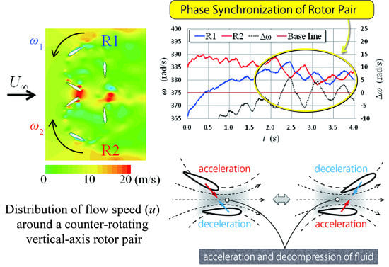[13] performed a CFD analysis on a rotating circular cylinder pair. The flow patterns around a circular cylinder pair might be analogous to the flow patterns around a turbine rotor pair in terms of spacing dependence. However, it is important to recognize the essential difference in the manner by which vortices are shed between a solid circular cylinder and a turbine rotor comprising blades. Recently, Vergaerde et al. [14] performed experiments using a closely spaced pair of straight-bladed VAWTs that mutually revolved in opposite directions in a wind tunnel and observed their phase synchronization. The first author of this paper and his colleagues have proposed a concept named “Wind Oasis” [15], which applies a wind farm comprising small-scale vertical-axis-type butterfly wind turbines (BWTs) [16] for agriculture in drylands to pump water for crops and to generate electricity for people. As basic studies for materializing this concept, the authors of the present paper have been conducting wind tunnel experiments using miniature BWT models and performing the 2D-CFD analysis of the corresponding rotors. Although not described in detail herein, Jodai et al. [17,18] observed phase synchronization in their experiments on a closely spaced miniature BWT pair as well.

In this study, to determine the optimal layout of a VAWT wind farm, a CFD analysis of a 2D vertical-axis rotor pair was performed considering the dynamic interaction between a fluid and wind turbines (i.e., the dynamic fluid-body interaction, DFBI [19]). In contrast to the aforementioned conventional CFD simulations, in this study, the rotational speed of each rotor was not fixed to a constant value but was simulated based on the equation of motion of the rotor. This CFD analysis using the DFBI is equivalent to experiments involving variable-speed wind turbines. Although some of the results have been reported in several oral presentations [20,21,22,23] and in a commentary article [15], they are integrated herein and new considerations and results are included; furthermore, the calculation times of some cases were prolonged until the rotor angular velocities converged within the new criteria. The details of the revised data acquisition are explained in the following section. The results were as follows. In the parallel layouts perpendicular to the main flow, the counter-down (CD) layouts (the blades move downwind in the gap) yielded a higher mean power than that of the counter-up (CU) layouts (the blades move upwind in the gap). By assuming an isotropic bidirectional wind speed, the co-rotating layouts (CO: two rotors in the parallel layout with the same rotational direction) were found to be superior to the combination of the CD and CU layouts in terms of mean output power at all gap lengths. In the tandem layouts along the main flow, the inverse-rotation (IR) configuration demonstrated an earlier recovery in terms of the mean rotor power in comparison with that of the CO configuration as the gap length increased. The analysis results of the 16-wind-direction configurations are discussed in detail. Finally, the phase synchronization of a rotor pair is demonstrated via CFD analysis and discussed.

2. Methods

In this study, a CFD analysis was performed using a 2D rotor, as shown in Figure 1b (hereinafter 2D-CFD rotor) as a target, which corresponds to the equator-level cross section of a 3D printed model, as shown in Figure 1a (hereinafter 3D-EXP rotor). The 3D-EXP rotor (diameter: D = 50 mm, height: H = 43.4 mm, chord length: c = 20 mm, blade cross section: NACA 0018) was used in the wind tunnel experiments performed in another study in parallel [17]. The 2D-CFD rotor did not include the hub and slant blade parts of the 3D-EXP rotor. The solidity of the 2D-CFD rotor used in this study was σ = Bc/(πD) = 0.38 (B: number of blades), which is larger than the solidity (σ = 0.10) of the rotor of Zanforlin and Nishino [7], that (σ = 0.15) of the rotor of Chen et al. [8], that (σ = 0.032) of the rotor of De Tavernier et al. [9], and that (σ = 0.176) of the rotor of Ma et al. [10]. The trailing edges of the blades of the 2D-CFD rotor were designed to be rounded with the curvature radius of 0.32 mm, in accordance with the 3D-EXP rotor.

In this study, the commercial application software STAR-CCM+ ver.14.04.011 was used as the numerical solver. The 2D unsteady incompressible Reynolds-averaged Navier-Stokes equations and the equation of continuity were solved by adopting the k–ω shear stress transport turbulence model [24]. A trim mesh was selected for the entire domain except for the region near the blade surfaces, where a prism layer mesh was used to create 15 layers that thinned progressively. The rotating motion of the rotor was realized using the overset mesh method. First, the torque performance (Q vs. ω; Q is the torque, and ω is the angular velocity) of an isolated single rotor was simulated at four wind speeds (U_∞ = 6, 8, 10, and 12 m/s). The entire calculation domain of the CFD analysis of the single rotor was a rectangle measuring 40D × 50D; the rotor center was positioned at 20D from the inlet boundary. Each run of the calculations were performed under a fixed rotational speed and was continued until the 10th rotor rotation was completed. The torque in the last five rotations of each run was averaged, and the results are shown in Figure 2.

The data depicted in Figure 2 were obtained by converting the 2D results into values corresponding to a 3D-EXP rotor. However, these data do not include the tip vortex loss and the effects of slant blades and a hub because of 2D-CFD. Therefore, in comparison with the measured torque performance [18] of the 3D-EXP rotor, the maximum torque depicted in Figure 2 was approximately 1.3 times larger, and the angular velocity corresponding to the maximum torque was approximately 1.5 times greater than the experimental data. Additionally, the torque performance in the low-angular-velocity region differed between the experimental and CFD results. However, the shapes of the torque curves obtained by the experiments and CFD analysis were typically similar in the regions around a torque peak and those of higher angular velocity.

The 2D calculation in STAR-CCM+ provided results that corresponded to the model with unit thickness, i.e., 1 m. Therefore, all the raw output values of the CFD analysis were multiplied by 0.0434, as shown in Figure 2, to convert them into torque values corresponding to those of the 3D-EXP rotor. The curve in red in Figure 2 represents the ideal load torque that passes a point that is 95% of the maximum power obtained via CFD analysis for a wind speed of 10 m/s. The load torque Q_L [N m] is expressed as follows:

$$Q_{\mathrm{L}}=3.71\times {10}^{-9}{\omega }^2$$

(1)

In the CFD analysis based on the DFBI method, the time-dependent angular velocity of each rotor is determined by solving the following equation of motion:

$$I\frac{d\omega }{dt}=Q_{\mathrm{R}}-Q_{\mathrm{L}}$$

(2)

In Equation (2), I is the moment of inertia of each rotor. When the mass of 3D-EXP rotor was assumed to be 14 g, the moment of inertia was estimated to be 5.574 × 10⁻⁶ kg m² based on a computer-aided design model. For the actual CFD analysis, the value of I = 5.574 × 10⁻⁶ kg m² × 1000 mm/43.4 mm = 1.284 × 10⁻⁴ kg m² was set in STAR-CCM+ because the 2D-CFD rotor had a unit length height. The Q_R term on the right-hand side of Equation (2) represents the rotational torque of each rotor obtained from CFD calculation. As for the load torque Q_L, the value of 1000/43.4 × Equation (1) (i.e., 8.55 × 10⁻⁸ ω²) was set in STAR-CCM+.

The parallel layouts of the two rotors, in which the line connecting the two rotor centers (y-axis direction) is perpendicular to the main flow (x-axis direction), include the three layouts shown in Figure 3a–c. In the CO layout (Figure 3a), the upper rotor (Rotor 1: R1) and lower rotor (Rotor 2: R2) rotate in the same direction; in the CD layout (Figure 3b), R1 and R2 rotate in different directions, and the blades move in the same direction as the main flow between the two rotor centers; in the CU layout (Figure 3c), the two rotors revolved in different directions and the blades moved against the main flow between the rotor centers. The terminology for the parallel layouts is based on De Tavernier et al. [9]. In this study, the CFD analysis was performed using the DFBI method (hereinafter DFBI-CFD) on a rotor pair comprising two 2D-CFD rotors in the aforementioned three parallel layouts, i.e., CO, CD, and CU, with different rotor spacings (gaps) of 10, 15, 25, 50,100, and 200 mm.

The tandem layouts of the two rotors, in which the line connecting the two rotor centers is parallel to the main flow direction, are classified into the two layouts shown in Figure 3d,e. In this study, the layouts shown in Figure 3d,e are classified as the tandem co-rotating (TCO) and tandem inverse-rotating (TIR) layouts, respectively. The DFBI-CFD analysis was performed for the TCO and TIR layouts with the gaps of 25, 50,100, 200, 300, 400, and 500 mm.

After executing the DFBI-CFD calculations for the parallel and tandem layouts, the 16-wind-direction configurations shown in Figure 4 were analyzed using similar methods. The cases shown in Figure 4a, in which two rotors rotate in the same direction, are defined as the CO configurations, whereas the cases shown in Figure 4b, in which two rotors rotate mutually in different directions, are termed as IR configurations in the present study. The coordinate system (x_R, y_R) depicted in Figure 4 is fixed at the rotor pair, and the origin is placed at the center of the rotor pair. The origin of the wind-direction angle θ is defined in the left-hand side of the rotor pair, i.e., as the direction of –x_R, in this analysis. For the five specific layouts shown in Figure 3, the CO layout corresponds to the case of θ = 0° in the CO configurations; the case of θ = 180° is identical to the CO layout and is not clearly indicated in Figure 4a; the TCO layout corresponds to the case of θ = 90° in the CO configurations; the case of θ = 270° is equivalent to the TCO layout, but the terms are not indicated in the same manner as that of the CO layout. The terms CD, CU, and TIR are shown in the corresponding parts in Figure 4b. It is clear from Figure 4 that the same layout exists in the symmetrical direction with respect to the center of the rotor pair (i.e., origin symmetry) in the CO configurations. By contrast, an equivalent case was observed in the symmetrical direction with respect to the x_R-coordinate axis (i.e., line symmetry) in the IR configurations. Therefore, the DFBI-CFD analysis was performed for approximately half of the cases of the 16-wind-direction configurations, and the results of the equivalent layout were substituted for those of the counterpart. The DFBI-CFD analysis for the 16-wind-direction configurations was conducted under the gaps of 25, 50, and 100 mm.

Figure 5 shows the mesh for the DFBI-CFD analysis of the rotor pair. The entire calculation domain was a rectangular region measuring 80D × 100D, and the center of the rotor pair was located at 40D from the inlet boundary. The mesh adopted for most parts of the entire domain was a trim mesh, and 15 layers of the prism layer mesh were created near the blade surfaces. The maximum value of y+, which is the non-dimensional distance of the first cell from the blade surface, was approximately 0.35 in any case. The overset mesh enabled the rotation of two rotors, even in the closest spacing of gap/D = 0.2. The number of cells in the static region was approximately 180,000, and that in two rotating regions added together was approximately 100,000; the total number of cells was approximately 280,000. The upstream uniform wind speed was fixed at U_∞ = 10 m/s for all simulations of the rotor pair. Owing to the interaction between the fluid and rotors, the rotational speed of each rotor varied based on the local flow condition as time progressed. When it was difficult to predict the converged value in advance, the initial angular velocity of each rotor was set to 366 rad/s, which was similar to the converged angular velocity ω_SI obtained in the DFBI-CFD analysis of an isolated single 2D-CFD rotor; when the converged angular velocity can be predicted, the value was set as the initial value. The initial phases of the two rotors in the CO layout shown in Figure 5b had a phase difference of π/3. However, for the other layouts, a unified initial phase condition was not set. Each calculation was performed until the results converged sufficiently; all the cases reported herein were calculated for 4 s at the least. The criterion of convergence was unified, i.e., when the root mean square (RMS) of the angular velocity in the final 1 s is less than 5 rad/s and the gradient of the linear approximation of the angular velocity in the final 1 s becomes less than 10 rad/s², then the DFBI-CFD simulation is stopped and the data such as the torque are averaged during the final 1s. The time step was 2.5 × 10⁻⁵ s. The Reynolds number based on the rotor diameter was Re = 3.3 × 10⁴, and that based on the blade chord length was approximately Re_b = 1.2 × 10⁴. As the boundary conditions, a constant flow velocity was assumed at the inlet and a constant gauge pressure (0 Pa) was maintained at the outlet. The slip condition was imposed on the side boundaries, whereas no-slip conditions were imposed on the blade surfaces.

The DFBI-CFD analysis of an isolated single rotor under U_∞ = 10 m/s yielded the following results as values equivalent to those of the 3D-EXP rotor: angular velocity, ω_SI = 366.1 rad/s (revolution per minute, N_SI = 3496 rpm); rotor torque, Q_SI = 0.485 mN m; output power, P_SI = 177.6 mW. In the following sections, the results of the rotor pair obtained from the DFBI-CFD analysis are expressed using the values divided by the single-rotor values, i.e., the normalized angular velocity ω_norm, normalized torque Q_norm, and normalized power P_norm.

3. Results and Discussion

In this section, results of the DFBI-CFD analysis on the rotor pair are presented and discussed. The following five Sections are presented: Section 3.1, gap dependence of parallel layouts; Section 3.2, gap dependence of tandem layouts; Section 3.3, gap and wind-direction dependence of the 16-wind-direction layouts; Section 3.4, comparison between CFD and experimental results; and Section 3.5, phase synchronization of the rotor pair.

3.1. Gap Dependence of Parallel Layouts

As examples of the CFD calculation for the parallel layouts, Figure 6a–c show the distributions of the x-direction component of flow velocity around a rotor pair with gap/D = 0.5, for CO, CD, and CU layouts. As shown in the CO layout in Figure 6a, the wake of each rotor deflected upward significantly. As shown in the CD layout in Figure 6b, the fluid accelerated considerably between the two rotors; the acceleration in the CU layout shown in Figure 6c was less than that in the CD layout.

In the red regions depicted in Figure 6, the flow speed is accelerated by the effects of vortices, although the figure does not directly indicate the vorticity. In the CD and CU layouts, the vortices are shed almost symmetrically with respect to the x-axis direction at the main flow; in contrast, in the CO layout, the vortex shedding exhibits asymmetry. Vortices are bound to a blade when the blade is in the upwind half and in the condition before shedding a strong vortex (i.e., a red-colored region). The bound vortices contribute to the generation of a lift force, that is, a rotational torque, by creating a circulation around the blade. The synthesis of the circulations arising from all the blades of each rotor generates a resultant circulation with a rotational direction identical to that of the rotor. The induced velocity caused by the circulation around each rotor, in a line-symmetrical manner, expands the wake in the CD layout (see Figure 6b) and narrows the wake in the CU layout (see Figure 6c). In contrast, in the CO layout depicted in Figure 6a, the wake is deflected on one side by the constructive superposition of the induced velocities of the two rotors because the circulations have the same direction.

The time variation in the angular velocity of each rotor in the parallel layouts (gap/D = 0.5) shown in Figure 6 is depicted in Figure 7 from the start of the calculation to 4 s. Figure 7 shows the results of the moving average based on a time width of 0.01 s. The initial value of all the cases shown in Figure 7 was 366 rad/s, which was similar to the converged angular velocity ω_SI of an isolated single rotor. As shown in Figure 6a, the two rotors in the CO layout rotated counterclockwise to the main flow emanating from the left-hand side, and the angular velocity of R2 increased owing to the induced velocity of R1, as shown in Figure 7a. Meanwhile, the angular velocity of R1, which was affected by the induced velocity of R2, did not decrease but increased slightly. As shown by the CD layout shown in Figure 7b, the angular velocities of the two rotors increased as much as that of R2 in the CO layout because the inflow to both rotors was enhanced by the mutual induced velocities. Because the direction of the induction in velocity in the CU layout shown in Figure 7c was opposite to that in the CD layout, the inflow to the rotors reduced. Therefore, the angular velocities of the two rotors were at the same level as the initial value or decreased slightly.

Figure 8 shows the gap dependence of the normalized angular velocity of each rotor in the CO, CD, and CU layouts. The white squares represent the average values of rotors R1 and R2. The angular velocity ω₂ of R2 was always larger than the angular velocity ω₁ of R1 in the CO layout, and the values of these two angular velocities were similar in the CD and CU layouts at any gap length. The magnitude relation of the angular velocities of R1 and R2, which are dependent on the layout, can be attributed to the symmetry or asymmetry of the vortex shedding and the superposition of the induced velocities caused by the circulation generated around each rotor (see Figure 6). Regardless of the layout type, as the gap decreased, the normalized angular velocity increased gradually until gap/D reached 0.5–1.0 and decreased rapidly after crossing the peak. This can be attributed to the blockage effects caused by gap narrowing, which is similar to the case of two closely spaced side-by-side circular cylinders. As the gap length approached zero, the rotor pair resembled a bluff body, and most of the inflow could not pass through the rotor gap region. Previous studies pertaining to two side-by-side circular cylinders indicated that the vortex shedding from a closely spaced cylinder pair was similar to that from a single-bluff-body, and that the mean drag coefficient of the cylinder pair increased as the gap narrowed [25]. Comparing the averaged values of the normalized angular velocities shown in Figure 8a–c, the relation CD > CO > CU was evident.

The gap dependence of the normalized torque shown in Figure 9 is more complicated than that of the angular velocity. In the CO layout, the mean torque Q₂ of R2 was greater than the mean torque Q₁ of R1 at all gap lengths. Moreover, the difference in the mean torques of the two rotors increased as the gap length decreased. However, Q₂ was not always greater than Q₁ when gap/D was varied in the CD and CU layouts. This was likely due to the dependence of the mean torque on the averaging period and timing, as the fluctuation in the torque was significant. The torque of R1 tended to decrease, and the torque of R2 abruptly increased as the gap became extremely small in the CO layout (Figure 9a). In the CD layout (Figure 9b), the averaged torque between Q₁ and Q₂ increased as the gap decreased until gap/D became 1.0, and as the gap space decreased after crossing the peak, the averaged torque decreased, whereas the torque of each rotor varied significantly. The average torque in the CU layout (Figure 9c) increased gradually until gap/D became 1.0 as the gap decreased, whereas it decreased abruptly when gap/D was less than 1. The rotation torque of a vertical-axis-type rotor depends significantly on the inflow angle and angle of attack, which are functions of the azimuth angle. The direction of flow (secondary flow) around the rotor significantly affects the torque behavior when the gap space is small.

The normalized power shown in Figure 10, which was obtained by multiplying the angular velocity and torque, indicates a gap dependence similar to that of the normalized torque shown in Figure 9. Considering the mean values of R1 and R2, the normalized power of the parallel layouts increased in the order of CD > CO > CU. This differs from the numerical results obtained by De Tavernier et al. [9] (σ = 0.032). It is unclear whether this was caused by the DFBI method. The results of the present DFBI-CFD analysis differed from the experimental results of Vergaerde et al. [14], where the relation CU > CD was obtained for a pair of two-bladed VAWT rotors with small solidity (the exact value is unknown). Although the experimental results using the 3D-EXP rotors (σ = 0.38) are not explained herein, the wind tunnel experiments showed the common relation CD > CU for the present numerical simulation. Furthermore, Zanforlin and Nishino [7] obtained the same relation (CD > CU) via CFD analysis using 2D rotors with σ = 0.102. The results above suggest that the rotor solidity might be related to the magnitude correlation pertaining to the power of the CD and CU layouts. An important finding is that the mutually counter-rotating rotor pair (the CD layout in this study) can yield a 23% higher average power than an isolated single rotor by approaching the two rotors to a distance of gap/D = 0.5–1, as shown in Figure 10b. This implies that, if the prevailing wind of a site has a high probability of appearance in a specific direction, appropriately installing a pair of VAWTs may generate more electricity than that expected from a single turbine. Moreover, as suggested by Dabiri [5], a wind farm comprising many VAWT pairs with the same appropriate configuration against the prevailing wind direction might achieve a high power density. However, further studies must be conducted for confirmation.

In comparison with the results reported previously [20], the results obtained in this study exhibit a better convergence in the CFD calculation. For example, the difference in power between R1 and R2 in the CO layout is depicted in Figure 10a.

A comparison between the normalized power in the CO layout and the averaged value of the normalized powers of the CD and CU layouts is tabulated in

Table 1. Averaged values of normalized powers under assumption of isotropic bidirectional wind speed.

Layout	gap/D = 0.2	gap/D = 0.3	gap/D = 0.5	gap/D = 1	gap/D = 2	gap/D = 4
CO	1.176	1.148	1.186	1.160	1.148	1.099
Ave. CD & CU	1.056	1.058	1.135	1.158	1.130	1.068

for each gap length. This corresponds to the comparison between the CO configuration and IR configuration, where a rotor pair is installed in a parallel layout under the assumption of an isotropic bidirectional wind speed. As shown in Table 1, the CO configuration yielded a higher output power than the IR configuration at any gap space in the ideal bidirectional wind condition.

3.2. Gap Dependence of Tandem Layouts

Examples of the DFBI-CFD results presented as color contours of flow velocity (x-direction component) around the tandem layouts are illustrated in Figure 11. Figure 11a,b show results of the TCO layouts; Figure 11c,d, the TIR layouts; Figure 11a,c, the case of gap/D = 1; and Figure 11b,d, the case of gap/D = 10. In the case involving a short gap length (Figure 11a,c), the downwind rotor R2 was almost completely within the wake of the upwind rotor R1. As the two rotors rotated in the same direction in the TCO layout shown in Figure 11a, the flow speed in the region below the rotor pair became higher than that in the region above because of the constructive interference caused by the induced velocities. In the case involving a long gap length (Figure 11b,d), although the effects of the wake of R1 on R2 became less prominent, part of the meandering wake of R1 flowed into R2.

Figure 12a,b show the gap dependence of the normalized angular velocity and normalized power of each rotor in the tandem layouts, respectively. As shown in Figure 12a, the angular velocity of the upwind rotor R1 was smaller than that of an isolated single rotor until the gap space reached gap/D = 8, indicating the effect of downwind rotor R2 on upwind rotor R1. Even in the case where the two rotors separated from each other and reached a length of gap/D = 10, the angular velocity of R2 was 70–80% that of an isolated single rotor, and the power was 40–50%. The 3D CFD analysis of a straight-bladed VAWT conducted by Miyashita et al. [26] demonstrated approximately 90% wake recovery at a distance of x/D ~ 5. Therefore, the slow recovery of the wake shown in Figure 12 is attributable to the 2D calculation. The gap dependence of the angular velocity and the power between the TCO and TIR layouts differed only slightly until gap/D = 6. Beyond gap/D = 8, however, the power of the downwind rotor R2 in the TIR layout became larger than that in the TCO layout. Comparing Figure 11b,d, it was observed that in the TCO layout, the induced velocity of the downwind rotor R2 (rotating counterclockwise) caused the upward-deflected wake of the upwind rotor R1 (rotating counterclockwise) in front of R2 to be drawn downward; meanwhile, in the TIR layout, as the induced velocity of R2 (rotating clockwise) deflected the wake of R1 further, the region with higher velocity flowed into R2.

In a previous report [22] on the wake of the tandem layouts where the calculation time was shorter, little difference was observed between the TCO and TIR. However, we observed a significant difference in the wake between the TCO and TIR in our study (see Figure 12b).

3.3. Gap and Wind-Direction Dependence of 16-Direction Layouts

The 16-wind-direction dependence of the normalized angular velocity in the CO and IR configurations with gap lengths of gap/D = 0.5, 1, and 2 are shown in Figure 13a–f. In each figure, the blue circles indicate the angular velocity ω₁ of R1, and the red triangle symbols the angular velocity ω₂ of R2. The white squares represent the mean values of both rotors. The green circle corresponds to the case of an isolated single rotor. In all the figures, the angular velocity of the downwind rotor R2 in the tandem layout of the wind direction of θ = 90° decreases significantly; similarly, that of the downwind rotor R1 in the tandem layout of θ = 270° decreased. In the case of gap/D = 0.5 (see Figure 13a,b), the extent of decrease in the angular velocity of the downwind-side rotor was the second largest in wind directions of θ = 112.5° and 292.5° in the CO configuration; meanwhile, it was the second largest for the tandem case in wind directions of θ = 112.5° and 247.5° in the IR configuration. This difference is attributed to the symmetry of the configurations, and in all the figures illustrating the distributions of the mean normalized angular velocity of the two rotors, the CO configuration exhibited the origin symmetry, whereas the IR configuration exhibited line symmetry with respect to the line connecting the wind directions of θ = 0° and 180°. In the case of gap/D = 1 shown in Figure 13c,d, the bias of distribution, i.e., the decrease in the angular velocity at θ = 112.5° and 292.5° observed in the case of gap/D = 0.5, reduced in the CO configuration; however, the bias was evident in the IR configuration. This is due to the significant wake deflection of the upwind rotor in the IR configurations, as shown by the comparison between Figure 11b,d. However, approaching gap/D = 2, the angular velocity distributions of both the CO and IR configurations exhibited similar shapes with less bias. This finding can be explained as follows: when the gap length became more than twice the rotor diameter, the downwind-side rotor located in the direction of Δθ = ±22.5° to the main flow was less affected by the wake of the upwind rotor in any configuration. Focusing on the neighborhoods of θ = 0° and 180°, as well as including the parallel layouts, in the CO configuration, the angular velocities in both neighborhoods were similar and larger than that of an isolated single rotor. Meanwhile, in the IR configuration, the angular velocities of R1 and R2 in the neighborhood of θ = 0° were higher than that of an isolated single rotor. However, in the neighborhood of θ = 180°, the angular velocities of both rotors were similar to that of an isolated single rotor, or the angular velocity of one rotor was higher than and that of the other rotor was lower than the angular velocity of an isolated single rotor.

The 16-wind-direction dependence of the normalized power shown in Figure 14 emphasizes the characteristics observed in Figure 13 for the distributions in the normalized angular velocity. Although the bias in the power distributions in the case of gap/D = 2 (Figure 14e,f) decreased compared with the case of a short gap, the distributions between the CO and IR configurations differed. In the CO configuration, the power of R2 was larger than that of R1 in wind directions of θ = 0°–67.5° (inversely, the power of R1 was larger than that of R2 in wind directions of θ = 180°–247.5°). Meanwhile, in the IR configuration, the power of R2 was larger than that of R1 in wind directions of θ = 135°–157.5° (inversely, the power of R1 was larger than that of R2 in wind directions of θ = 202.5°–225°).

A comparison of the 16-direction dependence of the mean normalized power of the two rotors is shown in Figure 15. Focusing on the neighborhoods of θ = 0° and 180°, as well as including the parallel layouts, in the CO configuration, the mean normalized powers in both neighborhoods were similar and exceeded that of an isolated single rotor, regardless of the gap space. The maximum rotor power averaged for three gap lengths was approximately 16% higher than the power of an isolated single rotor. In the IR configuration, the mean normalized powers in the neighborhood of θ = 0° were much higher than the power of an isolated single rotor (the maximum increase averaged for three gap lengths was approximately 22%). However, in the neighborhood of θ = 180°, the mean normalized power barely exceeded the power of an isolated single rotor (the maximum increase averaged for three gap lengths was approximately 6%). The power distributions in the CO and IR configurations for gap/D = 2 exhibited similar shapes and slight bias, except for the neighborhoods of θ = 0° and 180°.

The gap length dependence of the 16-wind-direction distribution of the average-normalized power reported in reference [15] appears to be consistent with the results of this study (see Figure 15). However, there were certain clear differences. For example, in the previous study, the average-normalized power in the CO layout (θ = 0° in the CO configuration) when gap/D = 1 was greater than that when gap/D = 0.5, whereas the opposite trend was observed in this study. As in this example, the data obtained in this study were improved in some cases.

The simple average of the normalized powers of the 16 wind directions is tabulated for each gap length and configuration in

Table 2. Simple average of normalized powers under assumption of isotropic 16-directional wind speed.

Configuration	gap/D = 0.5	gap/D = 1	gap/D = 2
CO	0.909	0.945	0.976
IR	0.886	0.929	0.975

. These values correspond to the ratios of the expected output power per rotor to that of an isolated single rotor under the assumption of an isotropic 16-directional wind speed. The simply averaged power in the CO configuration was higher than that in the IR configuration, regardless of the gap length. The difference between the two configurations decreased as the gap space increased.

3.4. Comparison between CFD and Experimental Results

Although details of the wind tunnel experiments [27] conducted by our group are not described here, some of the experimental results are compared with the CFD results in this section. Figure 16 depicts the distributions of the normalized mean angular velocity measured by arranging two models with the same size as that of the 3D-EXP rotor shown in Figure 1a under the condition of gap/D = 1. The load of each experimental rotor was a direct-current (DC) motor with open terminals, and the load performance was different from that of the ideal load torque assumed in the present CFD analysis (see Figure 2). Additionally, the experimental results depicted in Figure 16 were measured at a wind speed of 14 m/s generated by the wind tunnel. The compared CFD results represent the normalized mean angular velocities of the two rotors (R1 and R2) (see Figure 13c,d). The experimental data indicate the origin symmetry of the CO configuration and the line symmetry of the IR configuration exhibited in the CFD results in Section 3.3. In the next paragraph, we compare the experimental and CFD results of the normalized mean angular velocity in specific wind directions.

As shown in the CO configurations of Figure 16a, the experimental and CFD results agreed well except at angles of 112.5° and 292.5°. In the experiments, the downwind rotor stopped rotating at angles of 112.5° and 292.5°; therefore, the normalized mean angular velocity was approximately 0.5. This implies that the wake of the 3D-EXP rotor on the upwind side was deflected more, owing to the 3D effects such as slant blades, than that of the 2D-CFD rotor. In the IR configurations depicted in Figure 16b, the normalized mean angular velocity measured in the experiments was shifted inside the reference circle corresponding to an isolated single rotor in all directions. This bias can be attributed to the somewhat higher measurement result of the based angular velocity (CO: ω_SI = 408 rad/s, IR: ω_SI = 437 rad/s) of an isolated single rotor, which was measured in each series of experiments. When this bias was ignored, the experimental and CFD results were consistent, except for the tandem layouts of 90° and 270°. In the IR configurations, the downwind rotor in the tandem layouts stopped rotating. Figure 16b indicates that the experimental normalized mean angular velocity in the CD layout (θ = 0°) is greater than that in the CU layout (θ = 180°), which is similar to the CFD results.

3.5. Phase Synchronization of Rotor Pair

Figure 17 shows the DFBI-CFD analysis results of angular velocities of two rotors in the CD layout with a gap length of gap/D = 0.2, where the initial angular velocities were set at different values (R1: ω₁ = 366 rpm; R2: ω₂ = 385 rpm). The broken line expresses the difference between the angular velocities of the two rotors, i.e., Δω = ω₁ − ω₂. After 2 s from the start of the calculation, the two angular velocities ω₁ and ω₂ showed similar values but begin to alternate in terms of the magnitude correlation. The angular velocity difference Δω varied by changing the sign at an almost constant period. This phenomenon corresponds to the phase synchronization observed experimentally by Vergaerde et al. [14] and Jodai et al. [17,18]; to the best of our knowledge, the results shown in Figure 17 are the first reproduction of the phase synchronization of two VAWT rotors via CFD analysis.

Although Figure 18 corresponds to the same CD layout with gap/D = 0.2, as shown in Figure 17, the values calculated using the identical initial value (366 rpm) for both rotors are shown in Figure 18, the data of which are equivalent to those shown in Figure 8b and Figure 9b. The green broken line shows the difference in the angular velocities of the two rotors, and the orange broken line shows the difference in the torques ΔQ = Q₁ − Q₂. The torque difference shown in Figure 18 was obtained using the moving average of the original torque data with a time width of 0.1 s because the torque fluctuation was severe. To be consistent with the averaging time width of the torque difference, the angular velocity difference is illustrated using the moving average processed with the same time width of 0.1 s, as in Figure 18. Both Δω and ΔQ varied by sign change at a constant period of approximately 0.7 s, and the phase of ΔQ resulted in Δω varying by π/2. A similar phenomenon was observed in the CU layout with gap/D = 0.2 and 0.3. The time period of the variations in Δω and ΔQ increased as the gap space widened. The period was approximately 1 s in the CU layout with gap/D = 0.3.

The angular velocities (ω₁ and ω₂) of the two rotors and the difference Δω are illustrated for the CD layout with gap/D = 0.3, as shown in Figure 19. The data shown in Figure 19 indicate the most significant fluctuation among the data managed in this study. The RMS of ω₁ in the final 1 s (14–15 s), in which the data for Figure 19 were averaged to obtain the converged results, was 4.42 rad/s, and the gradient of the linear approximation was −6.34 rad/s². In this example, the two angular velocities indicated almost similar values, but the angular velocity difference Δω did not exhibit regular periodicity. In fact, by observing the movements of the blades simulated from the DFBI-CFD analysis, a small in-phase time zone was observed. In other words, phase synchronization was not observed in the CD layout with gap/D = 0.3. As mentioned above, however, phase synchronization was observed in the case of gap/D = 0.3 of the CU layout. Vergaerde et al. reported the instability of phase synchronization in a CD layout compared with that in a CU layout in their experiments [14]. The difference in the torque behavior between the CD and CU layouts in the region of short gap length shown in Figure 9b,c might be ascribed to the instability of the CD layout.

Next, the mechanism of phase synchronization generation was considered. Figure 20 shows the color contour of the flow velocity (x-direction component) around the rotors in a state of phase synchronization in the CD layout with gap/D = 0.2, which corresponds to the data in Figure 17. As illustrated in Figure 20, the blades of the two rotors rotated in phase. The fluid accelerated in the area between the blades that approached the minimal gap between the two rotors. From this observation and based on Bernoulli’s law, the pressure was reduced in the area sandwiched by the approaching blades. Consequently, the approaching blades with some phase difference mutually generated attractive forces, as illustrated in Figure 21; a delayed blade was accelerated and a leading blade was decelerated; this state might alternate at a constant period. Consequently, variations occurred in the angular velocity and torque, as shown in Figure 17 and Figure 18.

4. Conclusions

In this study, computational fluid dynamics (CFD) simulations were performed for a two dimensional closely spaced vertical-axis wind turbine (VAWT) rotor pair using the dynamic fluid-body interaction (DFBI) method. The counter-down (CD) layout yielded a higher average power of the two rotors than the counter-up (CU) layout owing to the effects of induced velocity. The average power of the two rotors in the CD layout with gap/D = 0.5–1 was 23% higher than the power of an isolated single rotor. In the case involving a long gap in the tandem layouts, the downwind rotor in the tandem inverse-rotating (TIR) layout tended to generate more power than that in the co-rotating (TCO) layout. This is attributed to the wake deflection caused by the induced velocity of the downwind rotor. Under the assumption of a virtual isotropic wind speed distribution, the mean power generated in the co-rotation (CO) configuration was higher than that in the inverse-rotation (IR) configuration. When the gap space reached twice the rotor diameter, the 16-wind-direction distribution in terms of the averaged power of the two rotors in the CO and IR configurations became similar. The present study demonstrated the phase synchronization of two VAWT rotors via CFD analysis for the first time. In the synchronized state, the phase of torque difference between the two rotors investigated advanced that of the angular velocity difference by π/2. The mechanism of phase synchronization, as explained based on Bernoulli’s law, was attributed to the acceleration and decompression of fluid between mutually approaching blades.

However, the DFBI-CFD analysis conducted in this study is a 2D analysis that overestimates the performance of a 3D experimental rotor model and cannot consider 3D effects, such as tip loss. Moreover, its computational cost is high. To consider the 3D effects, further studies on the interactions between rotors are necessary. To achieve the final objective of determining the optimal layout of a VAWT wind farm, we intend to develop a low-cost method using a simple model based on the results obtained by the DFBI-CFD analysis in our future work.

References

1. Göçmen, T.; van der Laan, P.; Réthoré, P.-E.; Diaz, A.P.; Larsen, G.C.; Ott, S. Wind turbine wake models developed at the technical university of Denmark: A review. Renew. Sustain. Energy Rev. 2016, 60, 752–769. [Google Scholar] [CrossRef] [Green Version]
2. Shao, Z.; Wu, Y.; Li, L.; Han, S.; Liu, Y. Multiple Wind Turbine Wakes Modeling Considering the Faster Wake Recovery in Overlapped Wakes. Energies 2019, 12, 680. [Google Scholar] [CrossRef] [Green Version]
3. Rajagopalan, R.G.; Rickerl, T.L.; Klimas, P.C. Aerodynamic interference of vertical axis wind turbines. J. Propul. Power 1990, 6, 645–653. [Google Scholar] [CrossRef]
4. Whittlesey, R.W.; Liska, S.; Dabiri, J.O. Fish schooling as a basis for vertical axis wind turbine farm design. Bioinspiration Biomim. 2010, 5, 035005. [Google Scholar] [CrossRef] [PubMed] [Green Version]
5. Dabiri, J.O. Potential order-of-magnitude enhancement of wind farm power density via counter-rotating vertical-axis wind turbine arrays. J. Renew. Sustain. Energy 2011, 3, 043104. [Google Scholar] [CrossRef] [Green Version]
6. Kinzel, M.; Mulligan, Q.; Dabiri, J.O. Energy exchange in an array of vertical-axis wind turbines. J. Turbul. 2012, 13, N38. [Google Scholar] [CrossRef]
7. Zanforlin, S.; Nishino, T. Fluid dynamic mechanisms of enhanced power generation by closely spaced vertical axis wind turbines. Renew. Energy 2016, 99, 1213–1226. [Google Scholar] [CrossRef] [Green Version]
8. Chen, W.-H.; Chen, C.-Y.; Huang, C.-Y.; Hwang, C.-J. Power output analysis and optimization of two straight-bladed vertical-axis wind turbines. Appl. Energy 2017, 185, 223–232. [Google Scholar] [CrossRef]
9. De Tavernier, D.; Ferreira, C.; Li, A.; Paulsen, U.S.; Madsen, H.A. Towards the understanding of vertical-axis wind turbines in double-rotor configuration. J. Phys. Conf. Ser. 2018, 1037, 022015. [Google Scholar] [CrossRef] [Green Version]
10. Ma, Y.; Hu, C.; Li, Y.; Li, L.; Deng, R.; Jiang, D. Hydrodynamic Performance Analysis of the Vertical Axis Twin-Rotor Tidal Current Turbine. Water 2018, 10, 1694. [Google Scholar] [CrossRef] [Green Version]
11. Poguluri, S.K.; Lee, H.; Bae, Y.H. An investigation on the aerodynamic performance of a co-axial contra-rotating vertical-axis wind turbine. Energy 2021, 219, 119547. [Google Scholar] [CrossRef]
12. Bearman, P.W.; Wadcock, A.J. The interaction between a pair of circular cylinders normal to a stream. J. Fluid Mech. 1973, 61, 499–511. [Google Scholar] [CrossRef]
13. Yoon, H.S.; Chun, H.H.; Kim, J.H.; Ryong Park, I.L. Flow characteristics of two rotating side-by-side circular cylinder. Comput. Fluids 2009, 38, 466–474. [Google Scholar] [CrossRef]
14. Vergaerde, A.; De Troyer, T.; Kluczewska-Bordier, J.; Parneix, N.; Silvert, F.; Runacres, M.C. Wind tunnel experiments of a pair of interacting vertical-axis wind turbines. J. Phys. Conf. Ser. 2018, 1037, 072049. [Google Scholar] [CrossRef]
15. Hara, Y.; Jodai, Y. Study on Close Arrangement of Small Vertical Axis Wind Turbines. Turbomach 2021, 49, 13–21. [Google Scholar]
16. Hara, Y.; Tagawa, K.; Saito, S.; Shioya, K.; Ono, T.; Makino, K.; Toba, K.; Hirobayashi, T.; Tanaka, Y.; Takashima, K.; et al. Development of a Butterfly Wind Turbine with Mechanical Over-Speed Control System. Designs 2018, 2, 17. [Google Scholar] [CrossRef] [Green Version]
17. Jodai, Y.; Hara, Y.; Sogo, Y.; Marusasa, K.; Okinaga, T. Wind tunnel experiments on interaction between two closely spaced vertical axis wind turbines. In Proceedings of the 23rd Chu-Shikoku-Kyushu Branch Meeting, JSFM, Yamaguchi, Japan, 1–2 June 2019. [Google Scholar]
18. Jodai, Y.; Hara, Y. Wind tunnel experiments on interaction between two closely spaced vertical axis wind turbines in parallel arrangements. Fluid Dyn. Res. 2021. under review. [Google Scholar]
19. Zhang, Y.; Kim, B. A Fully Coupled Computational Fluid Dynamics Method for Analysis of Semi-Submersible Floating Offshore Wind Turbines Under Wind-Wave Excitation Conditions Based on OC5 Data. Appl. Sci. 2018, 8, 2314. [Google Scholar] [CrossRef] [Green Version]
20. Yamamoto, S.; Hara, Y.; Jodai, Y. Numerical analysis on dynamic interaction between two closely spaced vertical axis wind turbines. In Proceedings of the 57th Chugoku-Shikoku Branch Meeting, JSME, Ube, Japan, 7 March 2019. [Google Scholar]
21. Okinaga, T.; Hara, Y.; Jodai, Y. Numerical analysis on the averaged power of a vertical axis wind turbine pair against 16-direction wind distributions. In Proceedings of the 2020 Annual General Meeting, JSME, Nagoya, Japan, (online). 16 September 2020. [Google Scholar]
22. Hara, Y.; Jodai, Y.; Yamamoto, S.; Okinaga, T. Numerical Simulation on Tandem Layout of Two Vertical Axis Wind Turbines. In Proceedings of the 2019 Annual General Meeting, JSME, Akita, Japan, 10 September 2019. [Google Scholar]
23. Hara, Y.; Jodai, Y.; Okinaga, T.; Sogo, Y.; Kitoro, T.; Marusasa, K. A synchronization phenomenon of two closely spaced vertical axis wind turbines. In Proceedings of the 25th Chu-Shikoku-Kyushu Branch Meeting, JSFM, Takamatsu, Japan, (online). 31 May 2020. [Google Scholar]
24. Menter, F.R. Two-equation eddy-viscosity turbulence models for engineering applications. AIAA J. 1994, 32, 1598–1605. [Google Scholar] [CrossRef] [Green Version]
25. Sumner, D. Two circular cylinders in cross-flow: A review. J. Fluids Struct. 2010, 26, 849–899. [Google Scholar] [CrossRef]
26. Miyashita, A.; Hara, Y.; Yoshida, S.; Sumi, T.; Akimoto, H. The effects of arms on the averaged wake of a straight-bladed vertical axis wind turbine with the inclined rotational axis. In Proceedings of the 50th Student Member Presentation of Graduation Theses, Chugoku-Shikoku Branch Meeting, JSME, Higashi-Hiroshima, Japan, 5 March 2020. [Google Scholar]
27. Sogo, Y.; Jodai, Y.; Hara, Y.; Kitoro, T.; Okinaga, T. Wind tunnel experiments on the rotational speed of a vertical axis wind turbine pair against 16-direction wind distributions. In Proceedings of the 59th Chugoku-Shikoku Branch Meeting, JSME, Okayama, Japan, (online). 5 March 2021. [Google Scholar]
Figure 1. Target rotors of this study: (a) 3D printed model (3D-EXP rotor); (b) 2D-CFD rotor used for CFD analysis.
Energies 14 02286 g001
Figure 2. Torque curves of 2D-CFD rotor and ideal load torque curve. Values of torque were converted to corresponding values of 3D-EXP rotor.
Energies 14 02286 g002
Figure 3. Specific layouts of a pair of VAWT rotors: (a) co-rotating (CO) layout; (b) counter-down (CD) layout; (c) counter-up (CU) layout; (d) tandem co-rotating (TCO) layout; (e) tandem inverse-rotating (TIR) layout.
Energies 14 02286 g003
Figure 4. Definition of 16-wind-direction configurations: (a) co-rotation (CO) configurations; (b) inverse-rotation (IR) configurations.
Energies 14 02286 g004
Figure 5. Calculation domain and mesh used in this study.
Energies 14 02286 g005
Figure 6. Color contours of flow velocity (x–direction component) when gap/D = 0.5: (a) CO layout; (b) CD layout; (c) CU layout.
Energies 14 02286 g006
Figure 7. Time variation of angular velocity of each rotor when gap/D = 0.5: (a) CO layout; (b) CD layout; (c) CU layout.
Energies 14 02286 g007
Figure 8. Gap dependence of normalized angular velocity of each rotor: (a) CO layout; (b) CD layout; (c) CU layout.
Energies 14 02286 g008
Figure 9. Gap dependence of normalized torque of each rotor: (a) CO layout; (b) CD layout; (c) CU layout.
Energies 14 02286 g009
Figure 10. Gap dependence of normalized power of each rotor: (a) CO layout; (b) CD layout; (c) CU layout.
Energies 14 02286 g010
Figure 11. Color contours of flow velocity (x−direction component): (a) TCO layout, gap/D = 1; (b) TCO layout, gap/D = 10; (c) TIR layout, gap/D = 1; (d) TIR layout, gap/D = 10.
Energies 14 02286 g011
Figure 12. Gap dependence of (a) normalized angular velocity and (b) normalized power of each rotor in tandem layouts.
Energies 14 02286 g012
Figure 13. 16-wind-direction dependence of normalized angular velocity: (a) CO configuration, gap/D = 0.5; (b) IR configuration, gap/D = 0.5; (c) CO configuration, gap/D = 1; (d) IR configuration, gap/D = 1; (e) CO configuration, gap/D = 2; (f) IR configuration, gap/D = 2.
Energies 14 02286 g013
Figure 14. 16-wind-direction dependence of normalized power: (a) CO configuration, gap/D = 0.5; (b) IR configuration, gap/D = 0.5; (c) CO configuration, gap/D = 1; (d) IR configuration, gap/D = 1; (e) CO configuration, gap/D = 2; (f) IR configuration, gap/D = 2.
Energies 14 02286 g014
Figure 15. 16-direction dependence of average of normalized power: (a) CO configuration; (b) IR configuration.
Energies 14 02286 g015
Figure 16. Comparison between CFD and experimental results on 16-wind-direction dependence of normalized mean angular velocity: (a) CO configuration, gap/D = 1; (b) IR configuration, gap/D = 1.
Energies 14 02286 g016
Figure 17. State of phase synchronization in angular velocities of two rotors in CD layout with gap/D = 0.2.
Energies 14 02286 g017
Figure 18. Phase shift between difference in angular velocities and that in torques, of two rotors in phase synchronization for CD layout with gap/D = 0.2 (data do not correspond to Figure 17 but Figure 8b and Figure 9b).
Energies 14 02286 g018
Figure 19. Out-of-phase state for angular velocities of two rotors in CD layout with gap/D = 0.3.
Energies 14 02286 g019
Figure 20. Color contour of flow velocity (x-direction component) around rotors in CD layout with gap/D = 0.2, where increase in flow speed by phase synchronization of two rotors is demonstrated.
Energies 14 02286 g020
Figure 21. Expected principle of phase synchronization in closely spaced wind turbines.
Energies 14 02286 g021