Impact of Lorentz Force in Thermally Developed Pulsatile Micropolar Fluid Flow in a Constricted Channel

Abstract

This work aimed to analyze the heat transfer of micropolar fluid flow in a constricted channel influenced by thermal radiation and the Lorentz force. A finite difference-based flow solver, on a Cartesian grid, is used for the numerical solution after transforming the governing equations into the vorticity-stream function form. The impact of various emerging parameters on the wall shear stress, axial velocity, micro-rotation velocity and temperature profiles is discussed in this paper. The temperature profile is observed to have an inciting trend towards the thermal radiation, whereas it has a declining trend towards the Hartman and Prandtl numbers. The axial velocity profile has an inciting trend towards the Hartman number, whereas it has a declining trend towards the micropolar parameter and Reynolds number. The micro-rotation velocity escalates with the micropolar parameter and Hartman number, whereas it de-escalates with the Reynolds number. The Nusselt number is observed to have a direct relationship with the Prandtl and Reynolds numbers.

1. Introduction

Micropolar (MP) fluids are non-Newtonian fluids consisting of a dilute suspension of an individual motion of thin, rigid cylindrical macromolecules. Incompressible MP fluids have significance in studying various phenomena, such as blood rheology in medical sciences and liquid crystal, and dilute solutions of polymer in industries. The MP fluid theory was first explained by Eringen [1]. Matiti [2] studied the free and forced convective heat transfer through the horizontal parallel plate channel. They concluded that the flow velocity increases both for heating and cooling. A two-dimensional incompressible magnetohydrodynamic (MHD) flow and heat transfer from electrically conducting micropolar fluid between two parallel porous plates was presented by Ojjela and Kumar [3]. They deduced that the temperature profile upsurges by increasing the Prandtl number. Perdikis and Raptis [4] analyzed the heat transfer in the steady flow of micropolar fluid past a plate and concluded that raising the radiation parameter causes an increase in the temperature profile. Gorla et al. [5] studied the steady heat transfer of an MP fluid over a semi-infinite flat plate. They deduced the result that thermal boundary layer thickness has an inverse relation with the Prandtl number. Makinde [6] inspected the impact of nonlinear convected heat on MHD boundary layer flow and melting heat transfer of an MP fluid with fluid particles suspended over a stretching surface. They discussed the effects of the emerging parameters on the momentum and thermal boundary layers, and the heat transfer rate. Turkyilmazoglu [7] investigated the MP fluid flow due to a permeable stretching sheet with heat transfer. He concluded that the decreasing value of the MP parameter results in an increase in the temperature profile. Ashraf and Wehgal [8] examined the incompressible laminar flow of an electrically conducting MP fluid between two porous disks. They deduced that the Nusselt number has a direct relationship with magnetic parameter, Reynolds number and Prandtl number. Rashidi [9] used the Homotopy analysis method to obtain accurate and complete analytic solutions of heat transfer of a micropolar fluid through a porous medium with radiation. The temperature profile decreases with increasing values of radiation parameter.

Hydrodynamical study of an MP fluid in a permeable channel was carried out by Lu [10]. The axial velocity has a declining behaviour towards the coupling number, whereas micro-rotation velocity has an inclining trend towards the coupling number. Javadi [11] examined the heat transfer of a two-dimensional MP fluid flow in a permeable channel using the variational iteration method (VIM). They deduced that the heat transfer rate upsurges as the Reynolds number increases. Doh et al. [12] studied the effect of heat generation on the fully developed flow of an MP fluid in a porous vertical channel. The temperature profile is higher for a low Reynolds number, in case of heating the fluid, as compared to for a high Reynolds number. A finite difference-based scheme was employed to examine the convective heat transfer of an MP fluid in a horizontal wavy channel with local heating by Miroshnichenko [13]. They concluded that a low Prandtl number forms a vortex in the channel, which results in a low heat transfer rate. Mekheimer [14] investigated the effect of induced magnetic field on peristaltic transport of an incompressible conducting MP fluid in a symmetric channel. The magnetic parameter had an inverse relation with the shear stress.

The study of the behaviour of human blood, as non-Newtonian fluid flow, through an artery having stenosis, plays an important role in understanding cardiovascular diseases. Young [15] studied the behaviour of flow in arteries having stenosis in detail. He discussed the flow separation region and profiles near the stenosis. Shit and Roy [16] examined the effects of magnetic field and heat on the pulsatile flow of blood taken as an MP fluid in the arteries with stenosis. Elahi et al. [17] studied the heat and mass transfer of MP fluid flow in arteries with mild stenosis having permeable walls. It was found that increasing values of coupling number and slip parameter result in a decrease in axial velocity profile. The temperature profile has a direct relation with the slip parameter, whereas it has an inverse relation with Darcy number. Haghighi and Asl [18] presented the mathematical modelling for two-dimensional pulsatile blood flow through overlapping constricted tapered vessels. They concluded that the taper angle has a direct relationship with velocity profile and volumetric flow rate, whereas it has an inverse relation with micro-rotation velocity. Ali et al. [19] investigated the impact of the magnetic field on the flow behaviour of a non-Newtonian Casson fluid in a constricted channel using Darcy’s law for the steady and pulsatile flows. The wall shear stress (WSS) had an inciting trend towards magnetic parameter, Strouhal number and Casson parameter. Further, the flow separation region could be controlled by the magnetic parameter. Bukhari et al. [20] expanded the study to analyze the heat transfer of Casson fluid in a constricted channel. The temperature profile had a declining trend towards the magnetic parameter, Casson parameter and Prandtl number, whereas it had an inciting trend towards the radiation parameter. Ali et al. [21] examined the pulsatile flow behaviour of micropolar-Casson fluid in a constricted channel. They concluded that the magnitude of micro-rotation velocity has a direct relation with the MP parameter, whereas it has an inverse relation with the Reynolds number.

The objective of the present study is to analyze the heat transfer effects in the pulsatile flow of an MHD MP fluid with thermal radiation in vessels having constricted walls. The model is solved using the finite difference method in the Cartesian coordinate system. The impact of different emerging parameters, such as the magnetic field parameter, Strouhal number (i.e., the flow pulsation parameter), micropolar parameter, Radiation parameter and Prandtl number on the flow profiles are explained graphically. The effects on the Nusselt number are examined, along with the wall shear stress, velocity, and temperature profiles. The flow separation region is also discussed near the stenosis with the help of streamlines. The rest of the paper is structured as follows. Section 2 describes the mathematical model and formulation. The results and discussions are presented in Section 3. Section 4 summarizes the conclusion.

2. Mathematical Formulation

2.1. Governing Equations

The pulsatile flow of an MP fluid in a channel with a pair of constrictions on the walls subject to Newtonian heating is considered (see Figure 1). A uniform magnetic field is applied perpendicular to the flow direction. The length of the constriction bump is $2x_0$, i.e., from $-x_0$ to $x_0$. The maximum channel width is set to be $L$. The induced electric field’s effect is considered negligible as the magnetic Reynolds number is very small.

The constrictions on the lower and upper walls of the channel are defined, in non-dimensional form, as:

$$\begin{array}{ccc}{y}_1\left(x\right)& =& \{\begin{array}{ll}\frac{h_1}{2}\left[1+\cos \left(\frac{\pi x}{x_0}\right)\right],\hfill & \left|x\right|\le x_0\hfill \\ 0, \hfill & \left|x\right|>x_0\hfill \end{array}\\ y_2\left(x\right)& =& \{\begin{array}{ll}1-\frac{h_2}{2}\left[1+\cos \left(\frac{\pi x}{x_0}\right)\right],\hfill & \left|x\right|\le x_0\hfill \\ 1, \hfill & \left|x\right|>x_0\hfill \end{array}\end{array}$$

(1)

The governing equations of the flow problem under consideration are given by:

$$\begin{array}{ccccccc}\frac{\partial \widehat{u}}{\partial \widehat{t}}+\widehat{u}\frac{\partial \widehat{u}}{\partial \widehat{x}}+\widehat{v}\frac{\partial \widehat{u}}{\partial \widehat{y}}& =& -\frac{1}{\rho }\frac{\partial \widehat{p}}{\partial \widehat{x}}+\left(\frac{\mu +k}{\rho }\right){\nabla }^2\widehat{u}+\frac{1}{\rho }{\left(J\times B\right)}_x+\frac{k}{\rho }\frac{\partial \widehat{N}}{\partial \widehat{y}}& & & & \end{array}$$

(2)

$$\begin{array}{ccccccccccc}\frac{\partial \widehat{v}}{\partial \widehat{t}}+\widehat{u}\frac{\partial \widehat{v}}{\partial \widehat{x}}+\widehat{v}\frac{\partial \widehat{v}}{\partial \widehat{y}}& =& -\frac{1}{\rho }\frac{\partial \widehat{p}}{\partial \widehat{y}}+\left(\frac{\mu +k}{\rho }\right){\nabla }^2\widehat{v}-\frac{k}{\rho }\frac{\partial \widehat{N}}{\partial \widehat{x}}& & & & & & & & \end{array}$$

(3)

$$\begin{array}{ccccccccccc}\frac{\partial \widehat{N}}{\partial \widehat{t}}+\widehat{u}\frac{\partial \widehat{N}}{\partial \widehat{x}}+\widehat{v}\frac{\partial \widehat{N}}{\partial \widehat{y}}& =& -\frac{k}{\rho j}\left(2\widehat{N}+\frac{\partial \widehat{u}}{\partial \widehat{y}}-\frac{\partial \widehat{v}}{\partial \widehat{x}}\right)+\frac{\gamma }{\rho j}{\nabla }^2\widehat{N}& & & & & & & & \end{array}$$

(4)

$$\begin{array}{ccccccccccccc}\frac{\partial \widehat{T}}{\partial \widehat{t}}+\widehat{u}\frac{\partial \widehat{T}}{\partial \widehat{x}}+\widehat{v}\frac{\partial \widehat{T}}{\partial \widehat{y}}& =& \frac{k}{\rho C_p}{\nabla }^2\widehat{T}-\frac{1}{\rho C_p}\frac{\partial q}{\partial \widehat{y}}& & & & & & & & & & \end{array}$$

(5)

$$\begin{array}{ccccccccccccccccccc}\frac{\partial \widehat{u}}{\partial \widehat{x}}+\frac{\partial \widehat{u}}{\partial \widehat{y}}& =& 0& & & & & & & & & & & & & & & & \end{array}$$

(6)

Here, the velocity components along $\widehat{x}$-axis and $\widehat{y}$-axis are represented by $\widehat{u}$ and $\widehat{v}$, respectively. $\rho$, $\widehat{p}$, $\nu$, and $\widehat{N}$ represent the density, pressure, kinematic viscosity, and angular velocity, respectively. $B\equiv \left(0,B_0,0\right)$, $J\equiv \left(J_x,J_y,J_z\right)$, and $\sigma$ represent the magnetic field with the uniform strength $B_0$ across the flow direction, the current density, and electric conductivity, respectively. $\gamma =j\left(\mu +k\right)/2$ is the spin gradient viscosity, $j$ and $\mu$ represent the micro inertia density and the dynamic viscosity, respectively. $k$ denotes the vortex viscosity and $q=-\left(\frac{4\sigma }{3k}\frac{\partial {\widehat{T}}^4}{\partial \widehat{y}}\right)$ represents the radiative heat flux. If $E\equiv \left(E_x,E_y,E_z\right)$ is the electric field and the direction of electric current flow is normal to the flow plane, then $E\equiv \left(0, 0,E_z\right)$. In addition, using Ohm’s law:

$$\begin{array}{cccccccccccccc}{J}_x=0,& J_y=0,& J_z=\sigma \left(E_z+\widehat{u}{B}_0\right)& & & & & & & & & & & \end{array}$$

(7)

Maxwell’s equation $\nabla \times E=0$ for steady flow implies that $E_z= a$, where $a$ is a constant number. We can assume a to be zero. Then, Equation (7) gives $J_z=\sigma \widehat{u}{B}_0$. Therefore, applying $J\times B=-\sigma \widehat{u}{B}_0^2$, Equation (2) becomes:

$$\begin{array}{cccccccc}\frac{\partial \widehat{u}}{\partial \widehat{t}}+\widehat{u}\frac{\partial \widehat{u}}{\partial \widehat{x}}+\widehat{v}\frac{\partial \widehat{u}}{\partial \widehat{y}}& =& -\frac{1}{\rho }\frac{\partial \widehat{p}}{\partial \widehat{x}}+\left(\frac{\mu +k}{\rho }\right){\nabla }^2\widehat{u}+\frac{-\sigma \widehat{u}{B}_0^2}{\rho }+\frac{k}{\rho }\frac{\partial \widehat{N}}{\partial \widehat{y}}& & & & & \end{array}$$

(8)

For Equation (5), expanding ${\tilde{T}}^4$ about $T_{\infty }$ (free stream temperature) and ignoring higher-order terms, we get:

$$\begin{array}{ccc}{\widehat{T}}^4& \cong & 4T_{\infty }^3\widehat{T}-3T_{\infty }^4\end{array}$$

Then $q=-\left(\frac{4\sigma }{3k}4T_{\infty }^3\frac{\partial \widehat{T}}{\partial \widehat{y}}\right)$ and $\frac{\partial q}{\partial \widehat{y}}=-\left(\frac{16\sigma }{3k}{T}_{\infty }^3\frac{{\partial }^2\widehat{T}}{\partial {\widehat{y}}^2}\right)$.

Equation $\left(5\right)$ becomes:

$$\begin{array}{cccccccccc}\frac{\partial \widehat{T}}{\partial \widehat{t}}+\widehat{u}\frac{\partial \widehat{T}}{\partial \widehat{x}}+\widehat{v}\frac{\partial \widehat{T}}{\partial \widehat{y}}& =& \frac{k}{\rho C_p}\left(\frac{{\partial }^2\widehat{T}}{\partial {\widehat{x}}^2}+\frac{{\partial }^2\widehat{T}}{\partial {\widehat{y}}^2}\right)+\frac{16\sigma T_{\infty }^3}{3k\rho C_p}\frac{{\partial }^2\widehat{T}}{\partial {\widehat{y}}^2}& & & & & & & \end{array}$$

(9)

The dimensionless form of Equations (3), (4), (6), (8), and (9) are obtained using the following:

$$\begin{array}{cccccccc}x=\frac{\widehat{x}}{L}, & y=\frac{\widehat{y}}{L},& u=\frac{\widehat{u}}{U},& v=\frac{\widehat{v}}{U},& t=\frac{\widehat{t}}{T},& p=\frac{\widehat{p}}{\rho U^2},& St=\frac{L}{UT},& Pr=\frac{\mu C_p}{k}, \\ N=\frac{\widehat{N}L}{U},& K=\frac{k}{\mu },& Re=\frac{UL}{\nu },& M=B_{0}L\sqrt{\frac{\sigma }{\rho \nu }},& \theta =\frac{\widehat{T}-T_2}{T_1-T_2},& Rd=\frac{16\sigma T_{\infty }^3}{3k\rho C_p}& \end{array}$$

(10)

Here $T$, $M$, $Re$, $St$, $Pr$, and $Rd$ represent the flow pulsation period, Hartman number, Reynolds number, Strouhal number, Prandtl number, and radiation parameter, respectively. $N$ denotes the micro-rotation velocity, and $K$ is the MP parameter.

Equations (8), (3), (4), (9), and (6) after transformation becomes:

$$\begin{array}{cccccccc}St\frac{\partial u}{\partial t}+u\frac{\partial u}{\partial x}+v\frac{\partial u}{\partial y}& =& -\frac{\partial p}{\partial x}+\left(\frac{1+K}{Re}\right){\nabla }^{2}u-\frac{M^2}{Re}u+\frac{K}{Re}\frac{\partial N}{\partial y}& & & & & \end{array}$$

(11)

$$\begin{array}{cccccccccc}St\frac{\partial v}{\partial t}+u\frac{\partial v}{\partial x}+v\frac{\partial v}{\partial y}& =& -\frac{\partial p}{\partial y}+\left(\frac{1+K}{Re}\right){\nabla }^{2}v-\frac{K}{Re}\frac{\partial N}{\partial x}& & & & & & & \end{array}$$

(12)

$$\begin{array}{ccccccc}St\frac{\partial N}{\partial t}+u\frac{\partial N}{\partial x}+v\frac{\partial N}{\partial y}& =& \frac{-K}{Re}\left(2N+\frac{\partial u}{\partial y}-\frac{\partial v}{\partial x}\right)+\left(\frac{1}{Re}+\frac{K}{2Re}\right){\nabla }^{2}N& & & & \end{array}$$

(13)

$$\begin{array}{cccccccccc}St\frac{\partial \theta }{\partial t}+u\frac{\partial \theta }{\partial x}+v\frac{\partial \theta }{\partial y}& =& \frac{1}{Re}\frac{1}{Pr}\left(\frac{{\partial }^2\theta }{\partial x^2}+\frac{{\partial }^2\theta }{\partial y^2}+Rd\frac{{\partial }^2\theta }{\partial y^2}\right)& & & & & & & \end{array}$$

(14)

$$\begin{array}{cccccccccccccccccc}\frac{\partial u}{\partial x}+\frac{\partial u}{\partial y}& =& 0& & & & & & & & & & & & & & & \end{array}$$

(15)

2.2. Vorticity-Stream Function Formulation

The vorticity $\left(\omega \right)$ and stream $\left(\psi \right)$ functions are given by:

$$\begin{array}{ccccccccccccc}u=\frac{\partial \psi }{\partial y}, & v=-\frac{\partial \psi }{\partial x},& \omega =\frac{\partial v}{\partial x}-\frac{\partial u}{\partial y}& & & & & & & & & & \end{array}$$

(16)

Some manipulations with Equations (11) and (12) produce:

$$\begin{array}{l}St\frac{\partial }{\partial t}\left(\frac{\partial v}{\partial x}-\frac{\partial u}{\partial y}\right)+u\frac{\partial }{\partial x}\left(\frac{\partial v}{\partial x}-\frac{\partial u}{\partial y}\right)+v\frac{\partial }{\partial y}\left(\frac{\partial v}{\partial x}-\frac{\partial u}{\partial y}\right)\\ =\left(\frac{1+K}{Re}\right)\left[\frac{{\partial }^2}{\partial x^2}\left(\frac{\partial v}{\partial x}-\frac{\partial u}{\partial y}\right)+\frac{{\partial }^2}{\partial y^2}\left(\frac{\partial v}{\partial x}-\frac{\partial u}{\partial y}\right)\right]-\frac{K}{Re}\left(\frac{{\partial }^{2}N}{\partial x^2}-\frac{{\partial }^{2}N}{\partial y^2}\right) \end{array}$$

(17)

The vorticity transport equation obtained using the quantities $\left(16\right)$, is given by:

$$\begin{array}{cc}St\frac{\partial \omega }{\partial t}+\frac{\partial \psi }{\partial y}\frac{\partial \omega }{\partial x}-\frac{\partial \psi }{\partial x}\frac{\partial \omega }{\partial y}=\left(\frac{1+K}{Re}\right)\left[\frac{{\partial }^2\omega }{\partial x^2}+\frac{{\partial }^2\omega }{\partial y^2}\right]+\frac{M^2}{Re}\frac{{\partial }^2\psi }{\partial y^2}-\frac{K}{Re}\left(\frac{{\partial }^{2}N}{\partial x^2}-\frac{{\partial }^{2}N}{\partial y^2}\right) & \end{array}$$

(18)

Again, using the quantities $\left(16\right)$, Equation $\left(13\right)$ becomes:

$$\begin{array}{cc}St\frac{\partial N}{\partial t}+\frac{\partial \psi }{\partial y}\frac{\partial N}{\partial x}-\frac{\partial \psi }{\partial x}\frac{\partial N}{\partial y}=\frac{-K}{Re}\left(2N+\frac{{\partial }^2\psi }{\partial x^2}+\frac{{\partial }^2\psi }{\partial y^2}\right)+\left(\frac{1}{Re}+\frac{K}{2Re}\right)\left(\frac{{\partial }^{2}N}{\partial x^2}-\frac{{\partial }^{2}N}{\partial y^2}\right)& \end{array}$$

(19)

And the Poisson equation for stream function $\psi$ is:

$$\begin{array}{cccccccccccccccc}\frac{{\partial }^2\psi }{\partial x^2}+\frac{{\partial }^2\psi }{\partial y^2}& =& -\omega & & & & & & & & & & & & & \end{array}$$

(20)

2.3. Boundary Conditions

Equation (2) assumes the following form the steady-state flow:

$$\begin{array}{ccccccccccccc}-\frac{1}{\rho }\frac{\partial \widehat{p}}{\partial \widehat{x}}+\left(\frac{\mu +k}{\rho }\right)\frac{{\partial }^2\widehat{u}}{\partial {\widehat{y}}^2}+\frac{1}{\rho }\left(J\times B\right)& =& 0& & & & & & & & & & \end{array}$$

(21)

Using $J\times B=-\sigma \left(E_z+\widehat{u}{B}_0\right)B_0$ in Equation $\left(21\right)$ gives:

$$\begin{array}{ccccccccccccc}\left(\frac{\mu +k}{\rho }\right)\frac{{\partial }^2\widehat{u}}{\partial {\widehat{y}}^2}-\sigma \widehat{u}{B}_0^2& =& \frac{\partial \widehat{p}}{\partial \widehat{x}}+\sigma E_z{B}_0& & & & & & & & & & \end{array}$$

(22)

Substituting the terms from Equation $\left(10\right)$ in Equation $\left(22\right)$ and performing some manipulations gives:

$$\begin{array}{ccccccccccccc}C\frac{d^{2}u}{d{y}^2}-M^{2}u& =& \frac{L^2}{\rho \nu U}\left(\frac{\partial \widehat{p}}{\partial \widehat{x}}+\sigma E_z{B}_0\right)& & & & & & & & & & \end{array}$$

(23)

where $\begin{array}{c}C=\left(1+K\right).\end{array}$ The solution of Equation $\left(23\right)$ is given by:

$$\begin{array}{cccccc}u\left(y\right)& =& \frac{1}{8}\left[\frac{\cosh \left(\frac{M}{2}\right)\left[\cosh \left(\frac{M}{2\sqrt{C}}\right)-\cosh \left(\frac{M}{\sqrt{C}}\left(y-\frac{1}{2}\right)\right)\right]}{{\sinh }^2\left(\frac{M}{4}\right)\cosh \left(\frac{M}{2\sqrt{C}}\right)}\right],& v=0,& M\ne 0& \end{array}$$

(24)

The inlet condition for the axial velocity with $M=0$ is given by:

$$\begin{array}{ccccccccccccc}u\left(y\right)=\frac{1}{C}\left(y-y^2\right),& & v=0,& & M=0,& & & & & & & & \end{array}$$

(25)

Equations $\left(24\right)$ and $\left(25\right)$ correspond to the steady velocity profile. A sinusoidal time-dependent expression is considered for the flow with pulsation:

$$\begin{array}{cccccccccccc}u\left(y,t\right)=u\left(y\right)\left[1+ϵ\sin \left(2\pi t\right)\right],& & v=0& & & & & & & & & \end{array}$$

(26)

At the walls, no-slip conditions are considered: $u=0,$ and $v=0$. The boundary conditions for $N$ on the walls are:

$$\begin{array}{cccccccccccccc}N={\left[-S\frac{\partial u}{\partial y}\right]}_{y=0,1}& \mathrm{with}& 0\le S\le 1& & & & & & & & & & & \end{array}$$

(27)

$S=0$, $S=\frac{1}{2},$ and $S=1$ represent the strong, weak and turbulent flow of concentrated particles near the walls in the fluid. The inlet condition for micro-rotation velocity is considered zero.

2.4. Transformation of Coordinates

The following relations are considered for the transformation of coordinates

$$\begin{array}{cccccccccccccc}\xi =x,& & \eta =\frac{y-y_1\left(x\right)}{y_2\left(x\right)-y_1\left(x\right)}& & & & & & & & & & & \end{array}$$

(28)

For computation purpose, we mapped the constriction to a straight channel, which results in mapping the domain $\left[y_1, y_2\right]$ to $\left[0, 1\right].$ Equations $\left(18\right)$, $\left(19\right)$, $\left(14\right)$ and $\left(20\right)$, applying Equation $\left(28\right)$, become,

$$\begin{array}{l}St\frac{\partial \omega }{\partial t}+u\left(\frac{\partial \omega }{\partial \xi }-Q\frac{\partial \omega }{\partial \eta }\right)+vD\frac{\partial \omega }{\partial \eta }\\ =\left(\frac{1+K}{Re}\right)\left[\frac{{\partial }^2\omega }{\partial {\xi }^2}-\left(P-2QR\right)\frac{\partial \omega }{\partial \eta }-2Q\frac{{\partial }^2\omega }{\partial \xi \partial \eta }+\left(Q^2+D^2\right)\frac{{\partial }^2\omega }{\partial {\eta }^2}\right]+\frac{D^2{M}^2}{Re}\frac{{\partial }^2\psi }{\partial {\eta }^2}\\ \hspace{1em}-\frac{K}{Re}\left[\frac{{\partial }^{2}N}{\partial {\xi }^2}-\left(P-2QR\right)\frac{\partial N}{\partial \eta }-2Q\frac{{\partial }^{2}N}{\partial \xi \partial \eta }+\left(Q^2+D^2\right)\frac{{\partial }^{2}N}{\partial {\eta }^2}\right] \end{array}$$

(29)

$$\begin{array}{l}St\frac{\partial N}{\partial t}+u\left(\frac{\partial N}{\partial \xi }-Q\frac{\partial N}{\partial \eta }\right)+vD\frac{\partial N}{\partial \eta }\\ =\frac{-K}{Re}\left[2N+\frac{{\partial }^2\psi }{\partial {\xi }^2}-\left(P-2QR\right)\frac{\partial \psi }{\partial \eta }-2Q\frac{{\partial }^2\psi }{\partial \xi \partial \eta }+\left(Q^2+D^2\right)\frac{{\partial }^2\psi }{\partial {\eta }^2}\right]\\ \begin{array}{ccccc}\hspace{1em}+\left(\frac{1}{Re}+\frac{K}{2Re}\right)\left[\frac{{\partial }^{2}N}{\partial {\xi }^2}-\left(P-2QR\right)\frac{\partial N}{\partial \eta }-2Q\frac{{\partial }^{2}N}{\partial \xi \partial \eta }+\left(Q^2+D^2\right)\frac{{\partial }^{2}N}{\partial {\eta }^2}\right]& & & & \end{array}\end{array}$$

(30)

$$\begin{array}{l}St\frac{\partial \theta }{\partial t}+u\left(\frac{\partial \theta }{\partial \xi }-Q\frac{\partial \theta }{\partial \eta }\right)+vD\frac{\partial \theta }{\partial \eta }\\ \hspace{1em}=\frac{1}{RePr}\left[\frac{{\partial }^2\theta }{\partial {\xi }^2}-\left(P-2QR\right)\frac{\partial \theta }{\partial \eta }-2Q\frac{{\partial }^2\theta }{\partial \xi \partial \eta }+\left(Q^2+D^2+Rd{D}^2\right)\frac{{\partial }^2\theta }{\partial {\eta }^2}\right]& & & & \end{array}$$

(31)

$$\begin{array}{cccccccc}\frac{{\partial }^2\psi }{\partial {\xi }^2}-\left(P-2QR\right)\frac{\partial \psi }{\partial \eta }-2Q\frac{{\partial }^2\psi }{\partial \xi \partial \eta }+\left(Q^2+D^2\right)\frac{{\partial }^2\psi }{\partial {\eta }^2}& =& -\omega & & & & & \end{array}$$

(32)

where

$$\begin{array}{ll}P=P\left(\xi ,\eta \right)=\frac{\eta y_2^{″}\left(\xi \right) + \left(1-\eta \right)y_1^{″}\left(\xi \right)}{y_2\left(\xi \right) - y_1\left(\xi \right)},& Q=Q\left(\xi ,\eta \right)=\frac{\eta y_2^{\prime }\left(\xi \right) + \left(1-\eta \right)y_1^{\prime }\left(\xi \right)}{y_2\left(\xi \right) - y_1\left(\xi \right)},\\ R=R\left(\xi \right)=\frac{y_2^{\prime }\left(\xi \right) - y_1^{\prime }\left(\xi \right)}{y_2\left(\xi \right) - y_1\left(\xi \right)},& D=D\left(\xi \right)=\frac{1}{y_2\left(\xi \right) - y_1\left(\xi \right)}\end{array}$$

(33)

The velocity components $u$ and $v$ become:

$$\begin{array}{cccccccccccc}u=D\left(\xi \right)\frac{\partial \psi }{\partial \eta },& & v=Q\left(\xi ,\eta \right)\frac{\partial \psi }{\partial \eta }-\frac{\partial \psi }{\partial \xi }& & & & & & & & & \end{array}$$

(34)

The boundary conditions at the walls, in the $\left(\xi ,\eta \right)$ coordinate system, for the stream, vorticity, micro-rotation velocity and temperature functions are:

$$\begin{array}{llll}\psi \left(\eta ,t\right)& =& \left[\frac{\sqrt{C}\cosh \left(\frac{M}{2}\right)\tanh \left(\frac{M}{2\sqrt{C}}\right)}{4M {\sinh }^2\left(\frac{M}{4}\right)}\right]\left[1+ϵ\sin \left(2\pi t\right)\right],& \mathrm{at} \eta =0 \\ \psi \left(\eta ,t\right)& =& \frac{\cosh \left(\frac{M}{2}\right)}{4{\sinh }^2\left(\frac{M}{4}\right)}\left[1-\frac{\sqrt{C}}{M}\tanh \left(\frac{M}{2\sqrt{C}}\right)\right]\left[1+ϵ\sin \left(2\pi t\right)\right],& \mathrm{at} \eta =1\end{array}$$

(35)

where the value of $ϵ$ determines the nature of the flow ($0$ for the steady case and 1 for the pulsatile case).

$$\begin{array}{l}\omega =-{\left[\left(Q^2+D^2\right)\frac{{\partial }^2\psi }{\partial {\eta }^2}\right]}_{\eta =0,1}\\ N=-{\left[w{D}^2\frac{{\partial }^2\psi }{\partial {\eta }^2}\right]}_{\eta =0,1}\end{array}$$

(36)

The boundary conditions for $\theta$ at the walls are as follows:

$$\begin{array}{cccccccccccc}\begin{array}{l}\theta =1, \mathrm{at} \eta =0\hfill \\ \theta =0, \mathrm{at} \eta =1\hfill \end{array}\}& & & & & & & & & & & \end{array}$$

(37)

The outlet boundary conditions for all the variables are associated with the fully developed flow. The dimensionless parameter Nusselt number, pertinent to the heat transfer analysis, is given by:

$$\begin{array}{cccc}Nu=\frac{L{q}_w}{k\left(T_1-T_2\right)}=-D\cdot {\theta }^{\prime }\left(0\right)& & & \end{array}$$

(38)

3. Results and Discussion

Equations $\left(29\right)$–$\left(32\right)$ are numerically solved using the alternating direction implicit (ADI) method [21] over a uniform structured grid spanned in $\xi$ and $\eta$ directions as follows: $\xi \in \left[-10,10\right]$ and $\eta \in \left[0,1\right]$. For the current study, a Cartesian grid of $400\times 50$ is used. The height and length of constriction on both walls are taken as $h=0.35$ and $x_0=2$, respectively. The value of $Re=700$ is fixed for all of the results obtained in this work unless stated otherwise. Equation $\left(32\right)$ is solved for $\psi =\psi \left(\xi ,\eta \right)$ and then Equations $\left(29\right)–\left(31\right)$ are solved for $\omega =\omega \left(\xi ,\eta \right)$, $N=N\left(\xi ,\eta \right)$, and $\theta =\theta \left(\xi ,\eta \right)$. The profiles of different parameters on the wall shear stress (WSS), axial velocity ($u$), micro-rotation velocity ($N$), temperature $\left(\theta \right)$ and Nusselt number ($Nu$) are computed. The profiles are shown at four different time levels defined as follows: $t=0.0$ stands for the start of pulsation motion; $t=0.25$ stands for the maximum flow rate; $t=0.50$ stands for minimum flow rate; and $t=0.75$ stands for the instantaneous zero flow rate. The expression of vorticity ($\omega$) is used to calculate the WSS since both are orthogonal to each other [22]. To save the wall-clock time, the solution can be obtained on high-performance parallel computers through parallelization of the code [23].

The $u$ profile and $N$ profile are shown in Figure 2 at the constriction’s throat (i.e., $x=0)$ with fixed values of $M=5$, $St=0.02$, $K=0.4$, $Pr=0.6$ and $Rd=0.7$. These profiles form regular fluctuating patterns due to the flow pulsation and exhibit higher escalations for larger distances from the walls. For validation, a strong agreement was established between the current work and Bandyopadhyay and Layek [24] for different values of $M$ with $N=K=0$, as shown in Figure 3.

The WSS on the upper wall of the channel for $M=0$, $5$, $10$ and $15$ is presented in Figure 4 at the four time instants of a pulse cycle. The WSS had an inciting trend towards $M$ and attains its maximum value at $t=0.25$. The flow decelerates during the interval of $0.25<t\le 0.75$. At $t=0.50$, the WSS was noted to have a declining trend towards $M$. Figure 5 presents the $u$ profile for $K=0.1$, $0.2$, $0.3$ and $0.4$. A symmetrical behaviour can be seen at the locations away from the constriction bump, e.g., $x=-5$ and $x=5$. The $u$ profile has an inciting trend towards $K$. At $t=0.25$, $u$ attains its peak value. Figure 6 presents the $u$ and $\theta$ profiles for $M=0$, $5$, $10$ and $15$ at $x=0$ and $x=2$ (constriction’s lee), respectively. The $u$ profile has an inciting trend towards $M$. The $u$ profile is maximum at the location $x=0$ at $t=0.25$. The thermal boundary layer shows a declining trend towards $M$. However, the fluctuations can be seen at $x=2$.

Figure 7 presents the WSS on the upper wall, $u$ and $\theta$ profiles for $St=0.02$, $0.04$, $0.06$ and $0.08$ at $x=0$. The WSS and $u$ profile have an inciting trend towards $St$ and attain the maximum value at $t=0.25$. The $\theta$ profile has a declining trend towards $St$. Figure 8 presents the WSS on the upper wall, $u$ and $\theta$ profiles for $K=0.1$, $0.2$, $0.3$ and $0.4$ at $x=0$. The WSS and $u$ profile have a declining trend towards $K$. The WSS and $u$ profile are maximum at $t=0.25$. There is no significant effect on the $\theta$ profile with increasing values of $K$ at $x=0$. Figure 9 depicts the WSS on the upper wall, $u$ and $\theta$ profiles for $Re=500$, $700$, $900$ and $1100$ at $x=0$. The WSS and thermal boundary layer have an inciting trend towards $Re,$ but $u$ profile has a declining trend towards $Re$.

Figure 10 presents the $\theta$ profile for $Pr=0.5$, $1.0$, $1.5$ and $2.0$ at $x=-2$, $x=0$ and $x=2$. The $\theta$ profile has a declining trend towards $Pr$. However, slight fluctuation near the lower wall can be seen. The Prandtl number is used to control the relative thickening of the momentum and thermal boundary layers. For small values of $Pr$, the heat transfer is quicker compared to velocity, which implies that the thermal boundary layer is thicker than the momentum boundary layer. Therefore, the cooling rate can be controlled by $Pr$. There is no effect on the WSS and $u$ profile with the variation of $Pr$. Figure 11 presents the $\theta$ profile for $Rd=0.4$, $0.8$, $1.5$ and $2.0$ at $x=-2$, $x=0$ and $x=2$. The $\theta$ profile has an inciting trend towards $Rd$. This behaviour verifies the physical fact that the thickness of the thermal boundary layer has a direct relation with $Rd$. There is no effect on the WSS and $u$ profile with the variation of $Rd$. Figure 12 depicts the impact of different values of $K$ on $N$ profile. The effect of $K$ on $N$ profile when $S=0$, i.e., micro-elements are close near the walls and unable to rotate, is shown in Figure 12a. The $N$ profile has an inciting trend towards $K$. Figure 12b presents the impact of $K$ on $N$ profile when $S=0.5$, i.e., weak concentration. Similar behaviour is seen in this case, as well. The influence of $Re$ on the $N$ profile is shown in Figure 13. Figure 13a depicts the effect of $Re$ on $N$ profile when $S=0$. The $N$ profile has a declining trend towards $Re$. Figure 13b presents the effect of $K$ on $N$ profile when $S=0.5$, i.e., weak concentration. Similar behaviour is seen in this case, as well.

Figure 14a,b present the effect of $Pr$ and $Re$ on the Nusselt number ($Nu)$. The $Nu$ has an inciting trend towards the $Pr$ and $Re$. Figure 15a presents the streamlines with the variation of $M$. It can be perceived that the streamlines are smooth near the constriction, and a decrease in the flow separation region can be observed with an increasing value of $M$. Figure 15b,c present the velocity and temperature contours, respectively. The ascending value of the magnetic parameter causes the increase in the size of temperature contours. Figure 16a presents the streamlines for different values of $St$. The streamlines are smooth, and there is no flow separation region. Figure 16b,c present the velocity and temperature contours, respectively. Ascending value of the Strouhal number causes an increase in the size of velocity contours.

Figure 17a presents the streamlines for variations of $Pr$. It is perceived that the streamlines are smooth near the constriction. Figure 17b,c present the velocity and temperature contours, respectively. The temperature contour density has an inciting trend towards $Pr$. Figure 18a presents the streamlines for different values of $Rd$. The streamlines are smooth near the constriction. Figure 18b,c present the velocity and temperature contours, respectively. The temperature contour density has a declining trend towards $Rd$.

4. Conclusions

The current work focuses on the heat transfer analysis of a micropolar fluid flow in a constricted channel under the impact of thermal radiation and the Lorentz force. The vorticity-stream function is used to transform the governing equations and then solved numerically by a finite difference based flow solver. Unlike the other studies in the literature, the solutions are computed on the Cartesian grid. The influence of different flow controlling parameters, including the Hartman number ($M$), Strouhal number ($St$), Prandtl number ($Pr$), micropolar parameter ($K$) and thermal radiation ($Rd$) parameters, on the WSS, axial velocity ($u$), micro-rotation velocity ($N$) and temperature ($\theta$) profiles were examined graphically. The streamlines, vorticity and temperature contours are also depicted. The key findings of the current work are as follows:

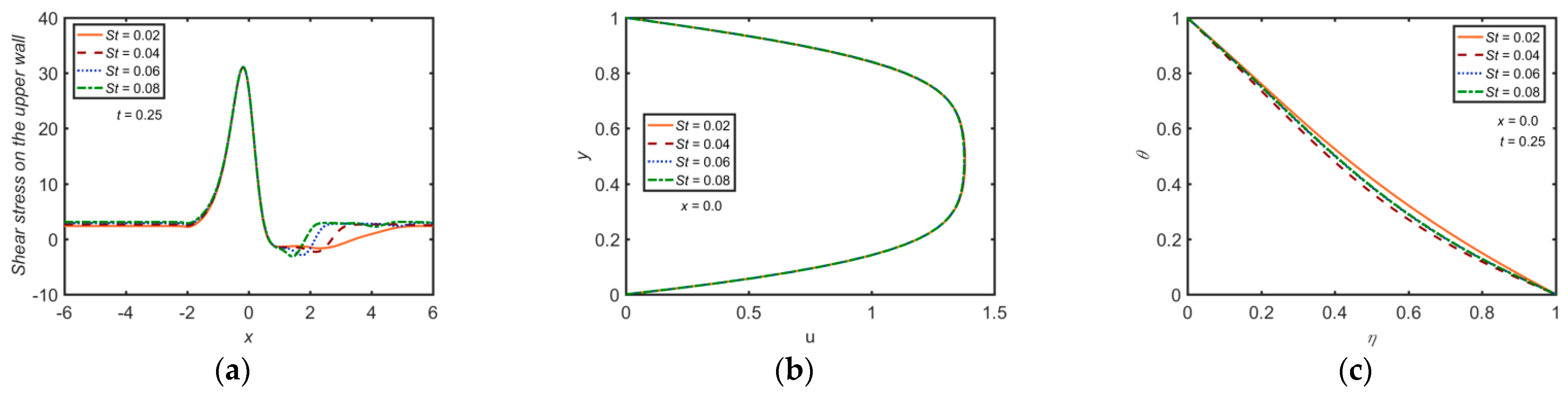
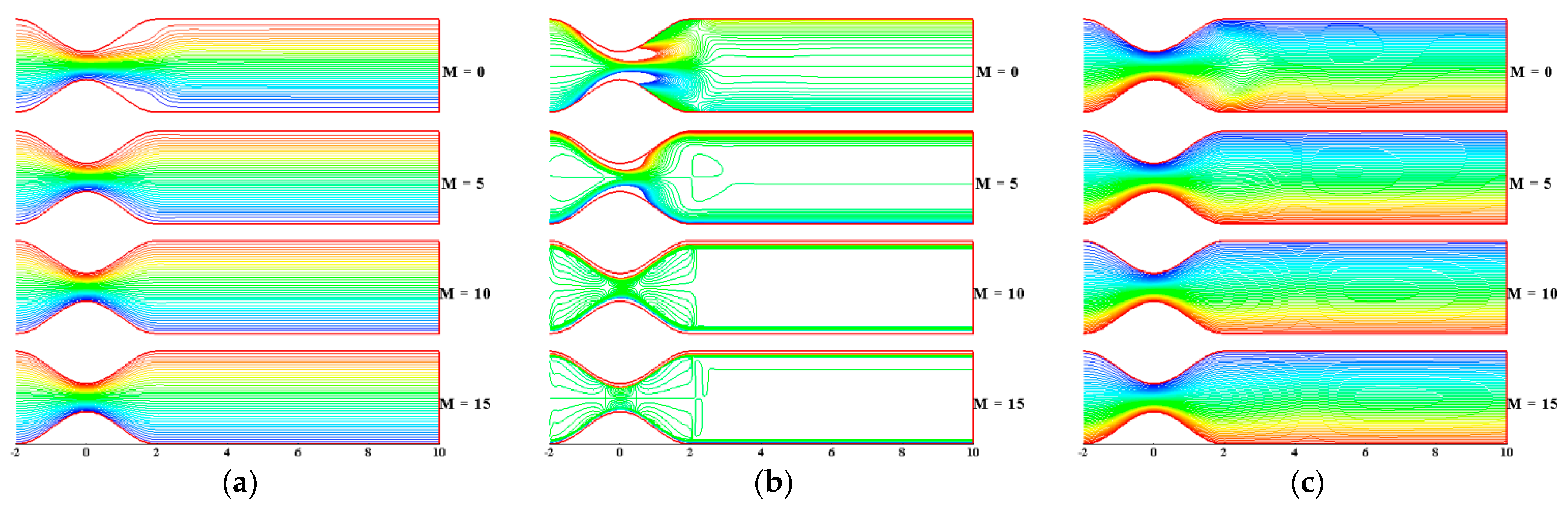
• The thermal boundary layer is observed to have an inverse relationship with the Hartman number and Prandtl number during the whole of the pulsation cycle.
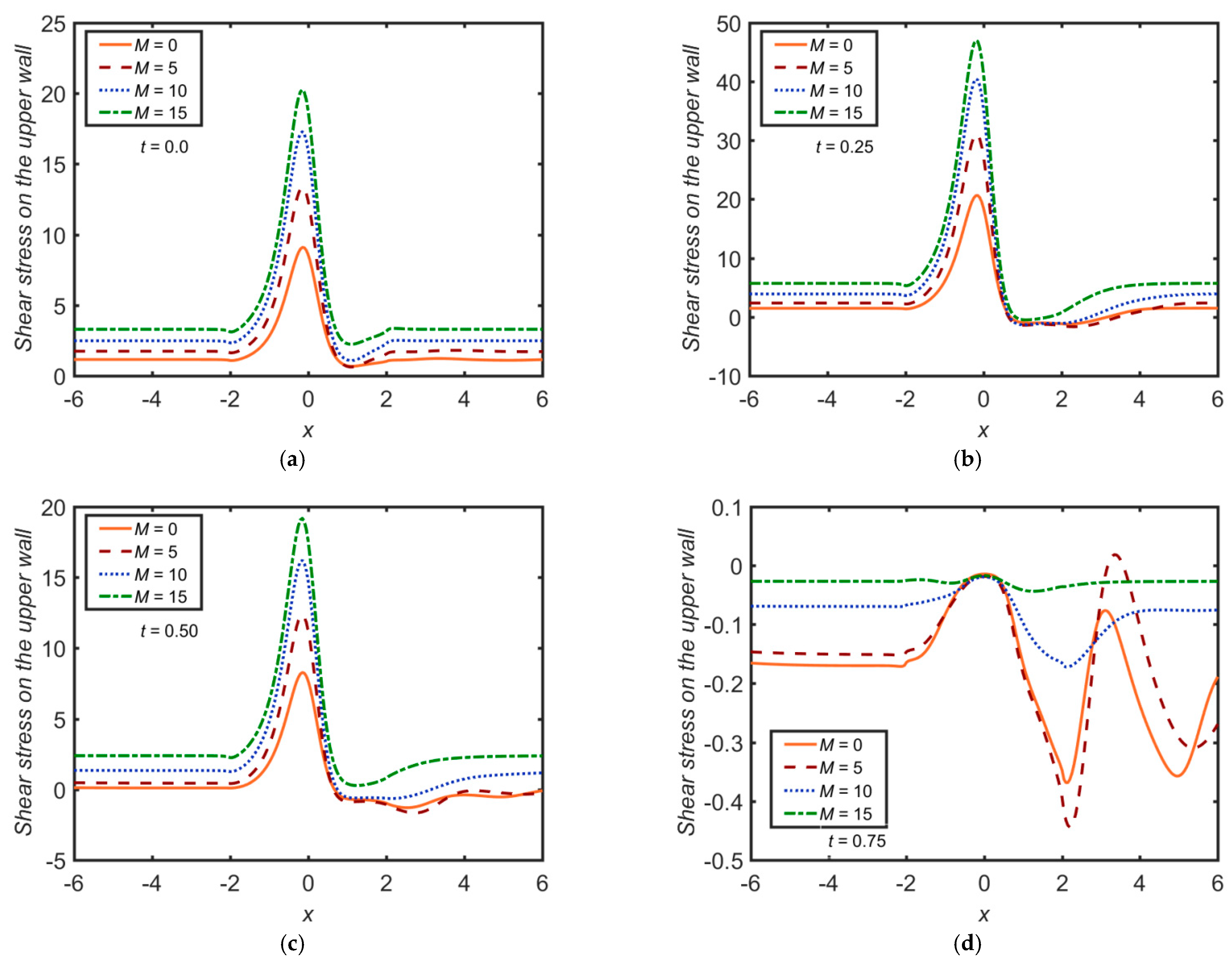
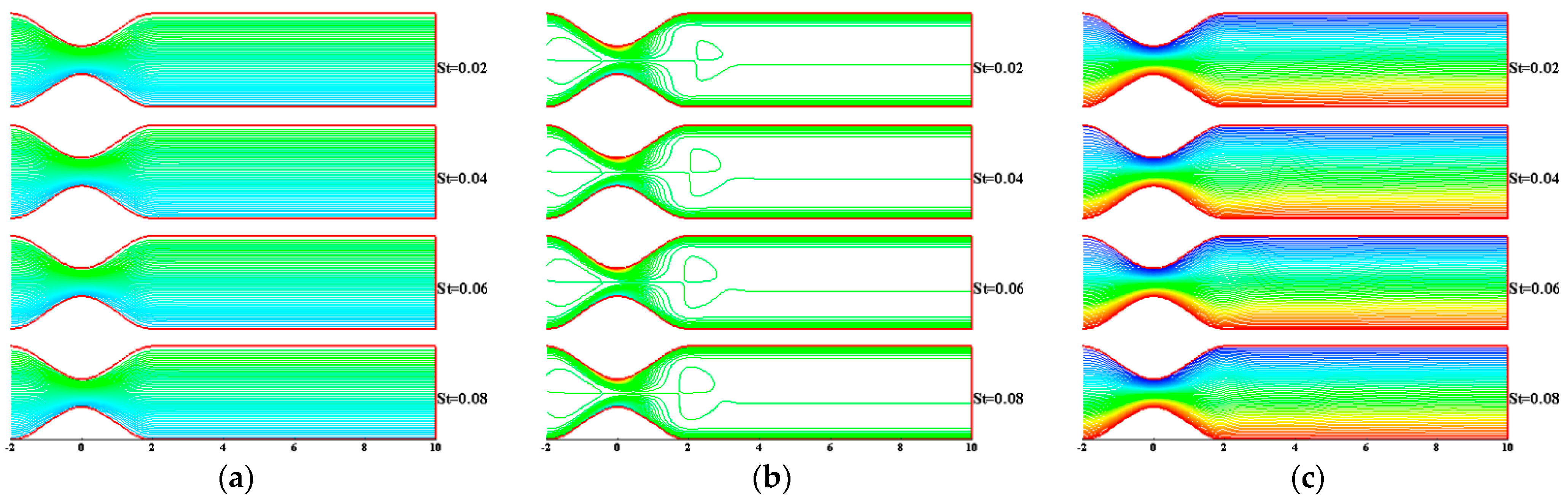
• The WSS has an inciting trend towards $M.$ At $t=0.25$, the WSS attains its peak value for a given value of $M$. Similar behaviour is seen on varying $St$ and $Re$. The WSS has a declining trend towards $K$. However, there is no effect of $Rd$ and $Pr$ on the WSS.
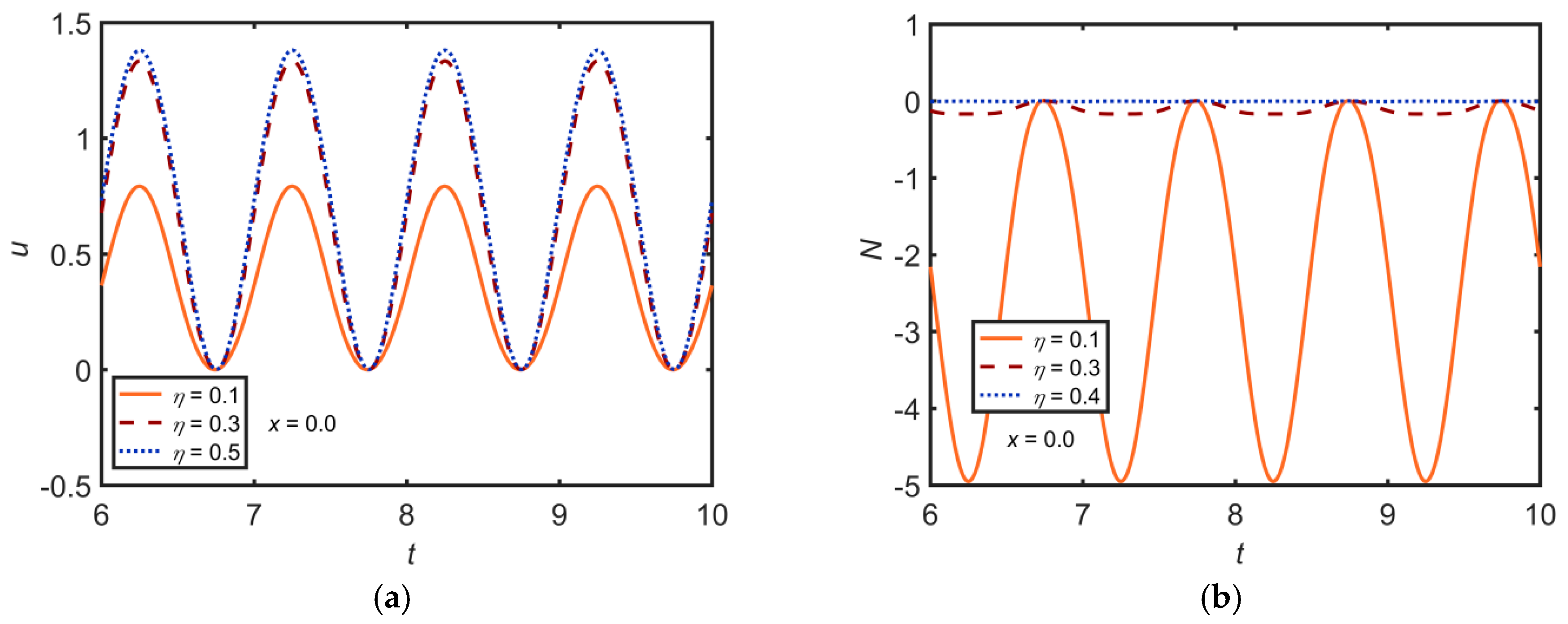
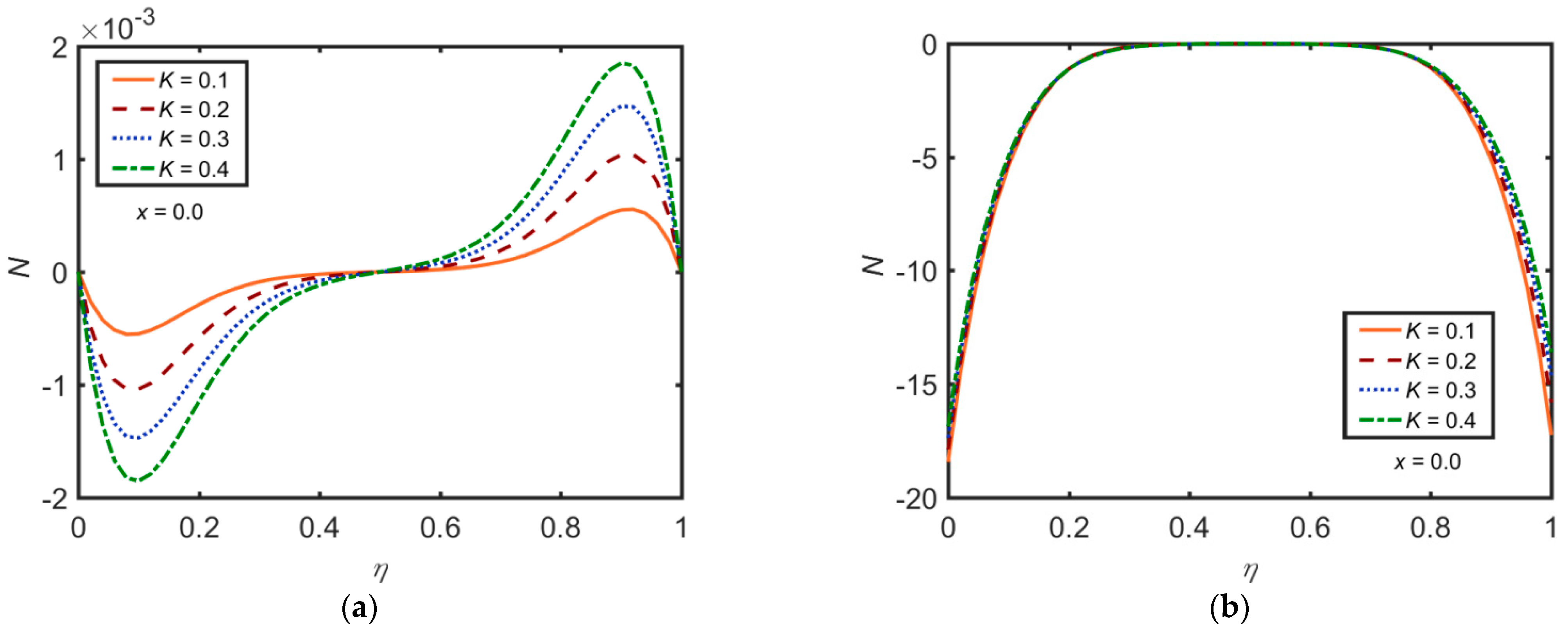
• The $u$ profile has an inciting trend towards $M$ and $St,$ but it has a declining trend towards $K$. There is no effect of $Rd$ and $Pr$ on the $u$ profile.
• The $N$ profile has an inciting trend towards $K$ and $M$, whereas a declining trend towards $Re$ is observed. No significant impact of other parameters on the $N$ profile is observed.
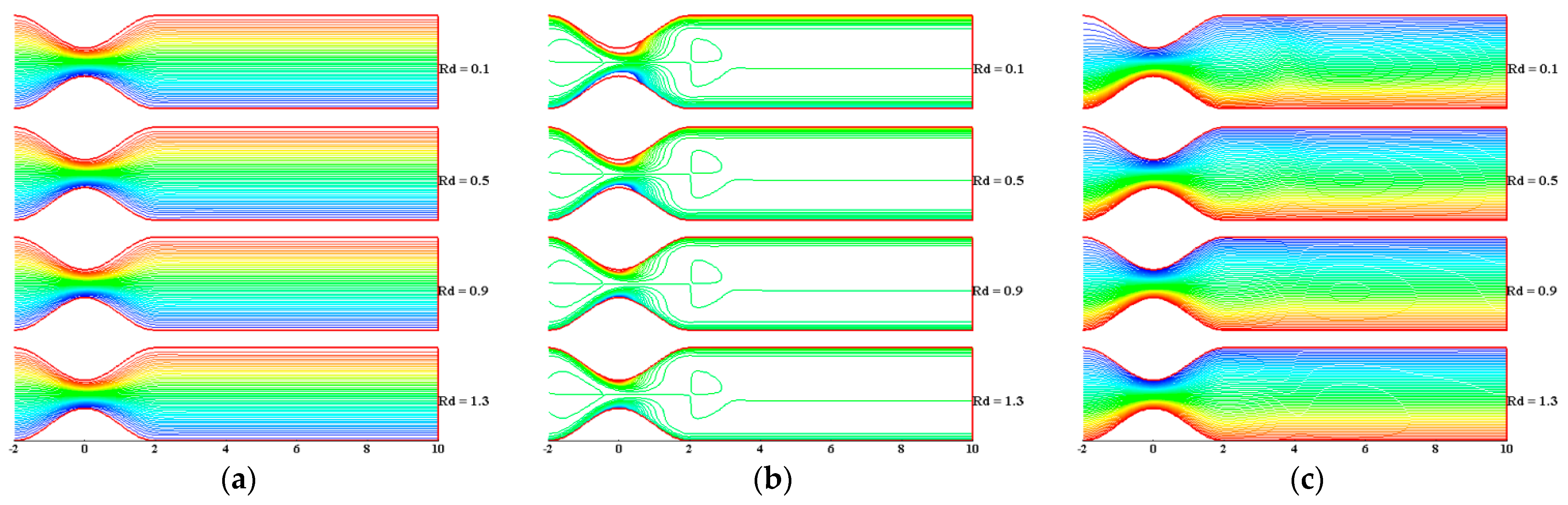
• The $\theta$ profile has a declining trend towards $M$, $St$, $Re$ and $Pr$. In contrast, it has an inciting trend towards $K$ and $Rd$. Since a declining trend in the $\theta$ profile towards $Pr$ is observed, it can be deduced that a thinner thermal boundary layer is caused due to a larger value of $Pr$.
• The dimensionless parameter $Nu$ has an inciting trend towards $Pr$ and $Re,$ whereas it has a declining trend towards $Rd$.

The finding of such a study might be helpful in the process of designing biomedical equipment for the treatment of cardiovascular diseases.

References

- Eringen, A.C. Simple microfluids. Int. J. Eng. Sci. 1964, 2, 205–217. [Google Scholar] [CrossRef]
- Maiti, G. Convective Heat Transfer in Micropolar Fluid Flow Through a Horizontal Parallel Plate Channel. ZAMM-J. Appl. Math. Mech. Z. Angew. Math. Mech. 1975, 55, 105–111. [Google Scholar] [CrossRef]
- Ojjela, O.; Naresh Kumar, N. Unsteady MHD flow and heat transfer of micropolar fluid in a porous medium between parallel plates. Can. J. Phys. 2015, 93, 880–887. [Google Scholar] [CrossRef]
- Perdikis, C.; Raptis, A. Heat transfer of a micropolar fluid by the presence of radiation. Heat Mass Transf. Stoffuebertragung 1996, 31, 381–382. [Google Scholar] [CrossRef]
- Gorla, R.S.R.; Pender, R.; Eppich, J. Heat transfer in micropolar boundary layer flow over a flat plate. Int. J. Eng. Sci. 1983, 21, 791–798. [Google Scholar] [CrossRef]
- Makinde, O.D.; Kumar, K.G.; Manjunatha, S.; Gireesha, B.J. Effect of nonlinear thermal radiation on MHD boundary layer flow and melting heat transfer of micro-polar fluid over a stretching surface with fluid particles suspension. Defect Diffus. Forum 2017, 378, 125–136. [Google Scholar] [CrossRef]
- Turkyilmazoglu, M. Flow of a micropolar fluid due to a porous stretching sheet and heat transfer. Int. J. Non-Linear Mech. 2016, 83, 59–64. [Google Scholar] [CrossRef]
- Ashraf, M.; Wehgal, A.R. MHD flow and heat transfer of micropolar fluid between two porous disks. Appl. Math. Mech. 2012, 33, 51–64. [Google Scholar] [CrossRef]
- Rashidi, M.M.; Mohimanian Pour, S.A.; Abbasbandy, S. Analytic approximate solutions for heat transfer of a micropolar fluid through a porous medium with radiation. Commun. Nonlinear Sci. Numer. Simul. 2011, 16, 1874–1889. [Google Scholar] [CrossRef]
- Lu, D.; Kahshan, M.; Siddiqui, A.M. Hydrodynamical study of micropolar fluid in a porous-walled channel: Application to flat plate dialyzer. Symmetry 2019, 11, 541. [Google Scholar] [CrossRef] [Green Version]
- Javadi, H. Investigation of micropolar fluid flow and heat transfer in a two-dimensional permeable channel by analytical and numerical methods. Sigma J. Eng. Nat. Sci. 2019, 37, 393–413. [Google Scholar]
- Doh, D.H.; Muthtamilselvan, M.; Prakash, D. Effect of heat generation on transient flow of micropolar fluid in a porous vertical channel. Thermophys. Aeromechanics 2017, 24, 275–284. [Google Scholar] [CrossRef]
- Miroshnichenko, I.V.; Sheremet, M.A.; Pop, I.; Ishak, A. Convective heat transfer of micropolar fluid in a horizontal wavy channel under the local heating. Int. J. Mech. Sci. 2017, 128–129, 541–549. [Google Scholar] [CrossRef]
- Mekheimer, K.S. Peristaltic flow of a magneto-micropolar fluid: Effect of induced magnetic field. J. Appl. Math. 2008, 2008. [Google Scholar] [CrossRef]
- Young, D.F. Fluid mechanics of arterial stenoses. J. Biomech. Eng. 1979, 101, 157–175. [Google Scholar] [CrossRef]
- Shit, G.C.; Roy, M. Pulsatile flow and heat transfer of a magneto-micropolar fluid through a stenosed artery under the influence of body acceleration. J. Mech. Med. Biol. 2011, 11, 643–661. [Google Scholar] [CrossRef]
- Ellahi, R.; Rahman, S.U.; Nadeem, S.; Akbar, N.S. Influence of heat and mass transfer on micropolar fluid of blood flow through a tapered stenosed arteries with permeable walls. J. Comput. Theor. Nanosci. 2014, 11, 1156–1163. [Google Scholar] [CrossRef]
- Haghighi, A.R.; Asl, M.S. Mathematical modeling of micropolar fluid flow through an overlapping arterial stenosis. Int. J. Biomath. 2015, 8, 1550056. [Google Scholar] [CrossRef]
- Ali, A.; Farooq, H.; Abbas, Z.; Bukhari, Z.; Fatima, A. Impact of Lorentz force on the pulsatile flow of a non-Newtonian Casson fluid in a constricted channel using Darcy’s law: A numerical study. Sci. Rep. 2020, 10, 1–15. [Google Scholar] [CrossRef]
- Bukhari, Z.; Ali, A.; Abbas, Z.; Farooq, H. The pulsatile flow of thermally developed non-Newtonian Casson fluid in a channel with constricted walls. AIP Adv. 2020, 11, 025324. [Google Scholar] [CrossRef]
- Ali, A.; Umar, M.; Bukhari, Z.; Abbas, Z. Pulsating flow of a micropolar-Casson fluid through a constricted channel influenced by a magnetic field and Darcian porous medium: A numerical study. Results Phys. 2020, 19, 103544. [Google Scholar] [CrossRef]
- Wu, J.Z.; Ma, H.Y.; Zhou, M.D. Vorticity and Vortex Dynamics; Springer Science and Business Media: Berlin, Germany, 2007. [Google Scholar]
- Ali, A.; Syed, K.S. An Outlook of High Performance Computing Infrastructures for Scientific Computing; Elsevier Inc.: Amsterdam, The Netherlands, 2013; Volume 91. [Google Scholar] [CrossRef]
- Bandyopadhyay, S.; Layek, G.C. Study of magnetohydrodynamic pulsatile flow in a constricted channel. Commun. Nonlinear Sci. Numer. Simul. 2012, 17, 2434–2446. [Google Scholar] [CrossRef]
Publisher’s Note: MDPI stays neutral with regard to jurisdictional claims in published maps and institutional affiliations. |
© 2021 by the authors. Licensee MDPI, Basel, Switzerland. This article is an open access article distributed under the terms and conditions of the Creative Commons Attribution (CC BY) license (https://creativecommons.org/licenses/by/4.0/).
Share and Cite
Umar, M.; Ali, A.; Bukhari, Z.; Shahzadi, G.; Saleem, A. Impact of Lorentz Force in Thermally Developed Pulsatile Micropolar Fluid Flow in a Constricted Channel. Energies 2021, 14, 2173. https://doi.org/10.3390/en14082173
Umar M, Ali A, Bukhari Z, Shahzadi G, Saleem A. Impact of Lorentz Force in Thermally Developed Pulsatile Micropolar Fluid Flow in a Constricted Channel. Energies. 2021; 14(8):2173. https://doi.org/10.3390/en14082173
Chicago/Turabian StyleUmar, Muhammad, Amjad Ali, Zainab Bukhari, Gullnaz Shahzadi, and Arshad Saleem. 2021. "Impact of Lorentz Force in Thermally Developed Pulsatile Micropolar Fluid Flow in a Constricted Channel" Energies 14, no. 8: 2173. https://doi.org/10.3390/en14082173
APA StyleUmar, M., Ali, A., Bukhari, Z., Shahzadi, G., & Saleem, A. (2021). Impact of Lorentz Force in Thermally Developed Pulsatile Micropolar Fluid Flow in a Constricted Channel. Energies, 14(8), 2173. https://doi.org/10.3390/en14082173