1. Introduction
Switching methods are widely used in electrical engineering for an energy efficient control of motors, DC or AC voltage supply units, or magnets. The historically oldest application of an energy efficient switching control is Montgolfier’s hydraulic ram from 1796 [
1]. Despite this historical lead role of hydraulics, the systematic study of switching controls in modern hydraulics started after the overwhelming success of this technology in electrical engineering became apparent and had the clear target to enable control without throttling and in a simpler way than with hydraulic transformers based on displacement machines. Since the early work by Brown and co-workers in the late eighties of the last century [
2,
3] numerous papers on “switched inertance” hydraulics—a term proposed by Nigel Johnston from Bath University—have been published. Ref. [
4] gives an overview of this work; [
5,
6,
7,
8,
9,
10,
11] are important contributions of recent years. In these cases, the inertia is realized by the fluid in a so-called inertance pipe. This is the simplest form but requires pipe lengths in the range of a meter or longer, depending on the switching frequency and required flow rate. The wave propagation processes in this pipe can lead to cavitation by standing waves [
12]. The coupling of inertia and resistance is strong which complicates the design of an effective inertance element. Another frequent realization of this element is to use a displacement machine, which runs as a pump and motor to which a flywheel is attached (e.g., [
13,
14]). Adjustment of the inertia is easy, which allows running smaller switching frequencies and using off the shelf on–off valves, but the displacement machine is a costly and bulky device and its fluctuating displacement properties may cause flow ripples and control problems at small flow rates. So far, work on switching control exploiting an oscillating heavy piston as an inertance element has been only published by the author’s workgroup. In the first publications [
15,
16], the converter was entitled “hydraulic resonance converter” because of its analogy to the electrical resonance inverter which is used for induction heating, sonar transmitters, fluorescent lighting, or ultrasonic generators [
17]. The schematic of a prototypal hydraulic converter to verify the working principle is shown in
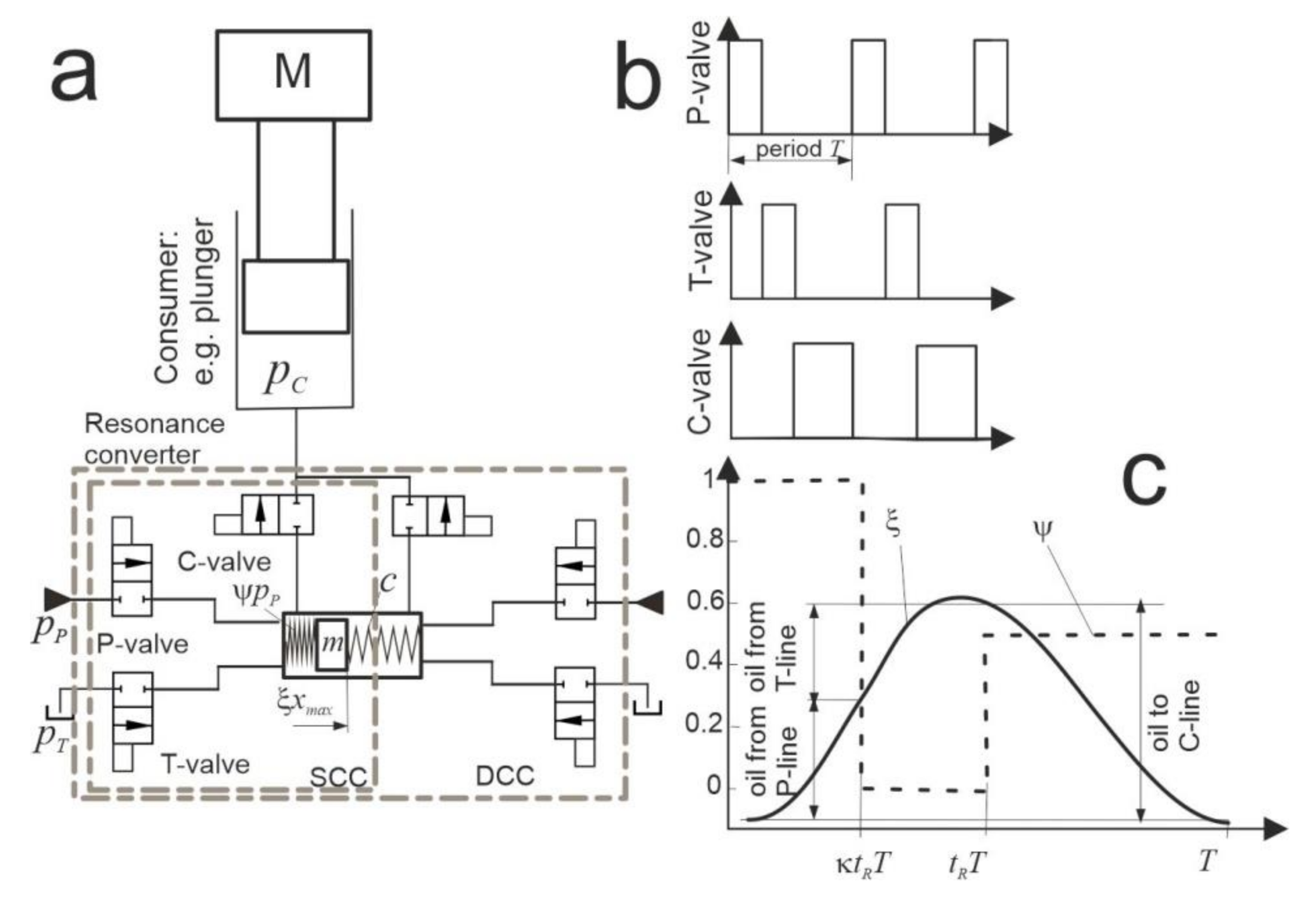
Figure 1. The low operating frequency in the range of 15 to 20 hertz, owing to the use of relatively slow proportional valves, led to a large system with a heavy mass of 20 kg. A large number of active valves is necessary to operate in all four quadrants. Off the shelf valves with a sufficient switching frequency in the range of at least 100 hertz, optimally 200 hertz, are not available and would definitely make the system rather expensive. The higher valve expense of this converter compared to inertance pipe or pump/motor type converters is compensated by a more compact design and the missing of complex wave propagation effects.
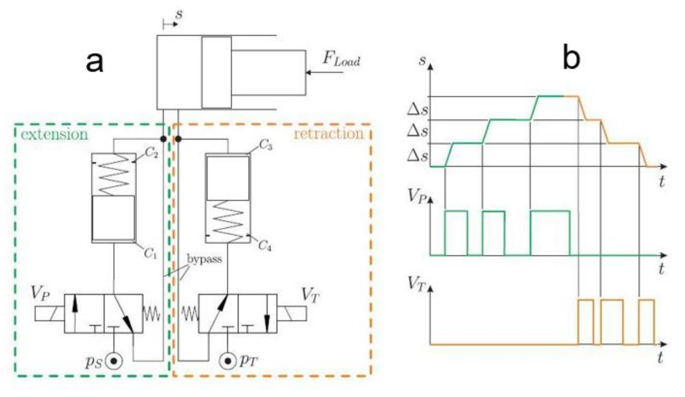
A second attempt to exploit an oscillating mass converter (OMC) aimed to realize a stepping control in an energy efficient manner [
18]. Its schematic is given in
Figure 2. A prototypal fast 3/2 way switching valve allowed running switching frequencies of 70 hertz, a prerequisite for a compact design. However, this and similarly performant valves are not available on the market. For the situation concerning availability of such valves, see [
19].
The cost of magnetically actuated valves is dominated by the solenoid. The costs percentage, disclosed informally by valve company representatives, is in the range 60% and more for conventional on–off valves. Fast switching valves for larger flow rates require higher dynamic performance. Hence, they are more costly and even worse, hardly available. Thus, the simplicity of electronic control of converters goes along with high costs and a very limited supply situation.
Mainly with the objective to realize high switching frequencies and large flow rates, several groups tested rotary valves [
20,
21]. Such valves are bulky, costly and not merchantable, hence, do not solve the cost and availability problem.
This paper presents a concept and an analysis by mathematical modeling and simulation of an OMC which employs pure hydraulic means for operation to overcome these cost and supply problems. To the best knowledge of the author, so far this approach has only been realized by the hydraulic ram but not in modern hydraulics. Functionally, the studied concept realizes a pressure relief valve since it controls the pressure at its input port (pressure pA) which is set hydraulically by a reference pressure pC. Its operating principle is a step-up converter since it transmits part of the incoming fluid to a high-pressure port (system pressure pP). Of course, this converter can also accomplish flow control if the actual flow rate is transformed into a pressure, e.g., by an orifice, which is compared to a reference pressure. This is a first feasibility study to find out if simple hydraulic concepts can provide high enough switching frequencies on the one hand and an acceptable control performance on the other hand.
2. The Oscillating Mass Converter
The basic idea of such converters is reflected in
Figure 1; the mass motion and valve timing diagrams show a step-down converter. The higher system pressure (
pP in
Figure 1) shall be transformed into a lower consumer pressure
pC without throttling, which requires that part of the outflow to the consumer comes from the tank line (pressure
pT). The piston is first accelerated by
pP by activating the P-valve and is then connected to the tank pressure to suck energetically free oil, approximately until it reaches its upper dead center. Then the energy delivered in the P-phase and stored in the compressed spring can be transferred to the consumer in the return motion (C-phase).
Operation as a step-up converter in only one power quadrant can be done in two modes. Both are sketched in
Figure 3. The converter includes a linear mechanical oscillator with a mass
m and a spring (constant
c) attached to a cylinder piston. The required values for
m at operating frequencies of approx. 100 hertz suggest a realization as a bulky element outside the cylinder. The cylinder can be of a single or double stroke type. The concept in
Figure 3 uses a single stroke cylinder.
In both operation modes, the first phase is a full stroke motion from upper to lower dead center in which the converter is connected to input port A (pressure
pA). The return motion has two phases: a P-phase and a T-phase. The two operation modes (APTM, ATPM) differ in the order of these two phases. The diagrams in
Figure 3 are valid for a periodic operation. Furthermore, they suggest that the PT transition in the APTM takes place at zero speed, which is a favorable situation since valve switching takes place at zero flow rate.
This converter has no energetic losses; if the fluid is incompressible, no pressure losses occur at the switching valve and the check valves, short circuiting between two of the three ports and leakage over the piston is avoided, and no mechanical friction brakes the oscillating motion. In reality, any of these conditions are violated; minimization of losses poses high performance requirements on the components and on control. Fast switching valves with large nominal flow rates reduce pressure losses, particularly also in the switching phases; a low friction guidance of the piston with low leakage keeps friction losses small (see [
18] for the significance of this effect); fast check valves prevent the backflow of fluid and the corresponding losses. With a very timely actuation of the valve, the compressibility losses can also be minimized. The latter measure, however, requires the 3-2 way valve being replaced by two 2-2 way valves, both with a very fast and accurate response. Such valve timing considerations have been extensively studied in [
16].
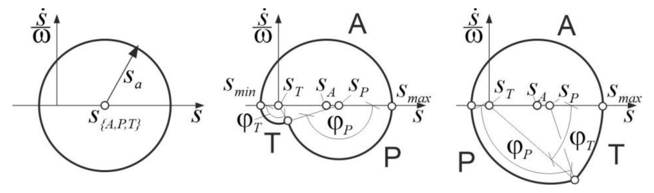
2.1. A Simple Model of the OMC
In order to obtain a compact understanding of the basic working principle, a simple model which reflects the idealized situation and enables a simple graphical representation is established. It is based on the linear equation of motion of the oscillator, neglecting friction, and the perfect working of the valves, which means that the pressure in the cylinder equals the pressure of the port when it is switched on. The equation reads:
Its solution is a harmonic oscillation around an offset value which depends on the actual phase. It lends itself for a complex number representation:
and to a corresponding graphical analysis, as shown in the next figure. Each phase is represented by a circular curve in the phase space located at one of the offset positions
s{A,P,T}.
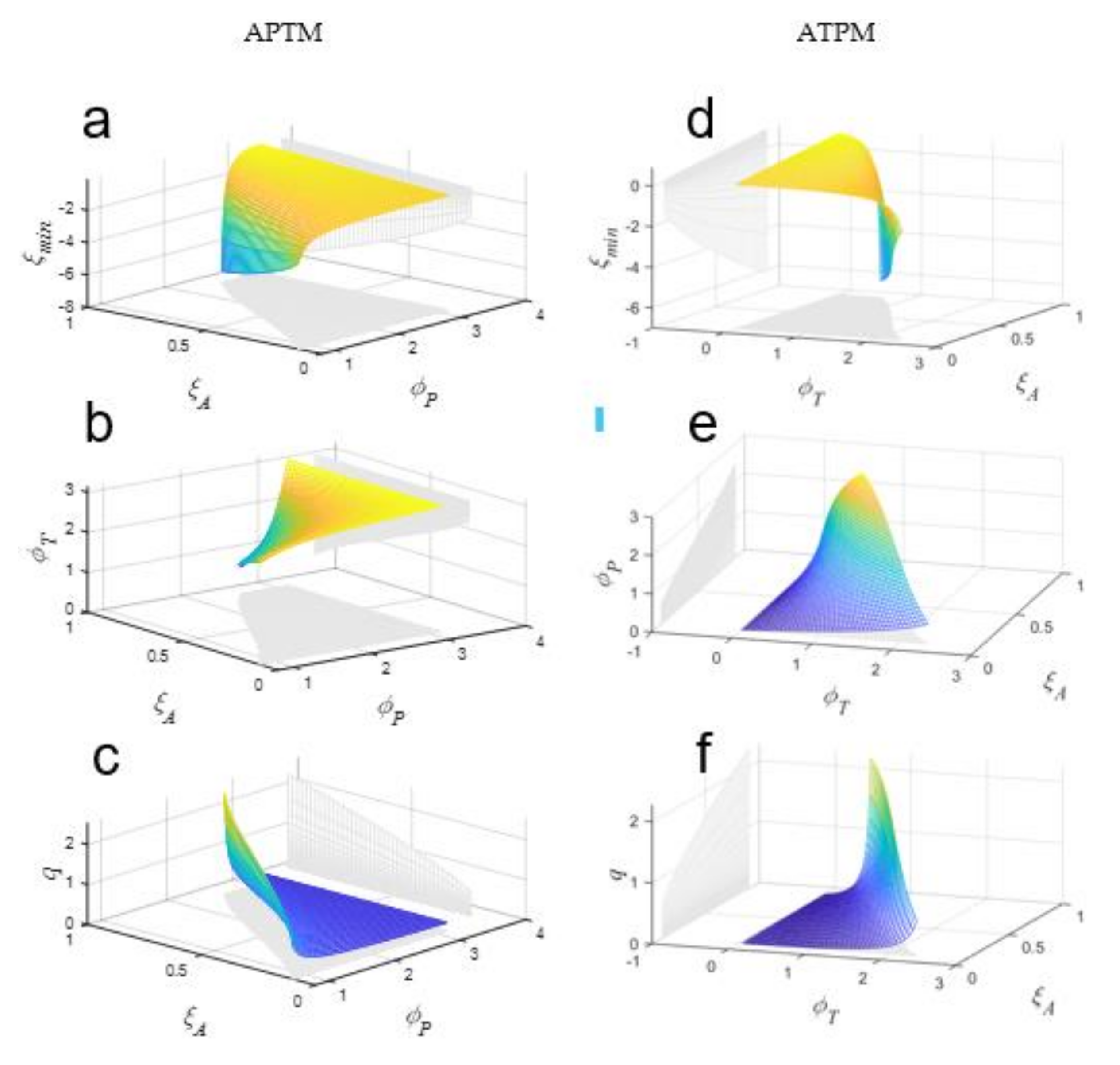
If the A-phase stretches over a half cycle (
φA = π) and for the steady state operation, the full cycle for both operation modes are given by a semicircle in the upper half plane and two circular arches in the lower half plane. The phase angles {
φA,
φP,
φT} correspond to the phase times {
tA,
tP,
tT} according to:
Transition between the P- and T-phase at zero speed (zero speed switching ZSW) is only possible for APTM;
φT = π,
φP = π and the full cycle time reads:
With the given port pressures for ZSW, the oscillation stroke and, in turn, the average flow rate
QA,aver from the input port are fixed and can be derived from
Figure 4:
This means that flow control by an uninterrupted operation of the three phases independent of the system pressure pP is impossible. In other words, flow control requires interruptions between two of the three phases.
ZSW is impossible for ATPM for step-up conversions, i.e.
sP > sA. For general switching (GSW), the relations can be easily derived from the geometric conditions in the phase space as sketched in
Figure 4. In these periodic cases, they are reflected by the following results, which, for compactness reasons, are given in nondimensional quantities:
The results are visualized in the following diagrams of
Figure 5.
2.2. Conclusions of the OMC Model Results
The diagrams for
ξmin and
q in
Figure 5 show a resonance effect for both operation modes which is exploited when the system is operated as a so-called resonance converter. The resonance line in the
ξA −
ξmin is given by the vanishing denominator in the equation for
ξmin.
Of course, the resonance peak depends strongly on the damping in the system, which is missing in the simple analytical model. Furthermore, it requires a precise control of switching, which could be done reasonably with fast and precise electrically actuated valves but is very challenging with hydraulically controlled valves.
The diagrams for both modes of operation are limited by the resonance line. Beyond this line, a useful operation is impossible.
ATPM can control the flow rate (q in the diagrams) from zero to a maximum value according to the resonance peak value, whereas APTM does not go below a minimum value q = 2/3π.
The main downside of ATPM is the need to switch the valve from state “1” to state “0” when the piston has a high speed. Since such processes need some time, additional losses, pressure ripples, and mechanical shocks are created. APTM switches at zero speed and is, therefore, selected for a realization by a pure hydraulic control concept. Of course, this is an idealized view according to the simplifications of the model used in this section. Fluid compressibility and the delayed switching of the real system (of the switching valve and of the check valve) cause a deviation from the ideal case and let the piston perform oscillations until the switching valve is switched to the tank line. However, the switching takes place at low piston speeds which strongly reduces the typical problems of switching at high speeds: pressure and flow peaks and mechanical shock.
3. Hydraulically Controlled OMC
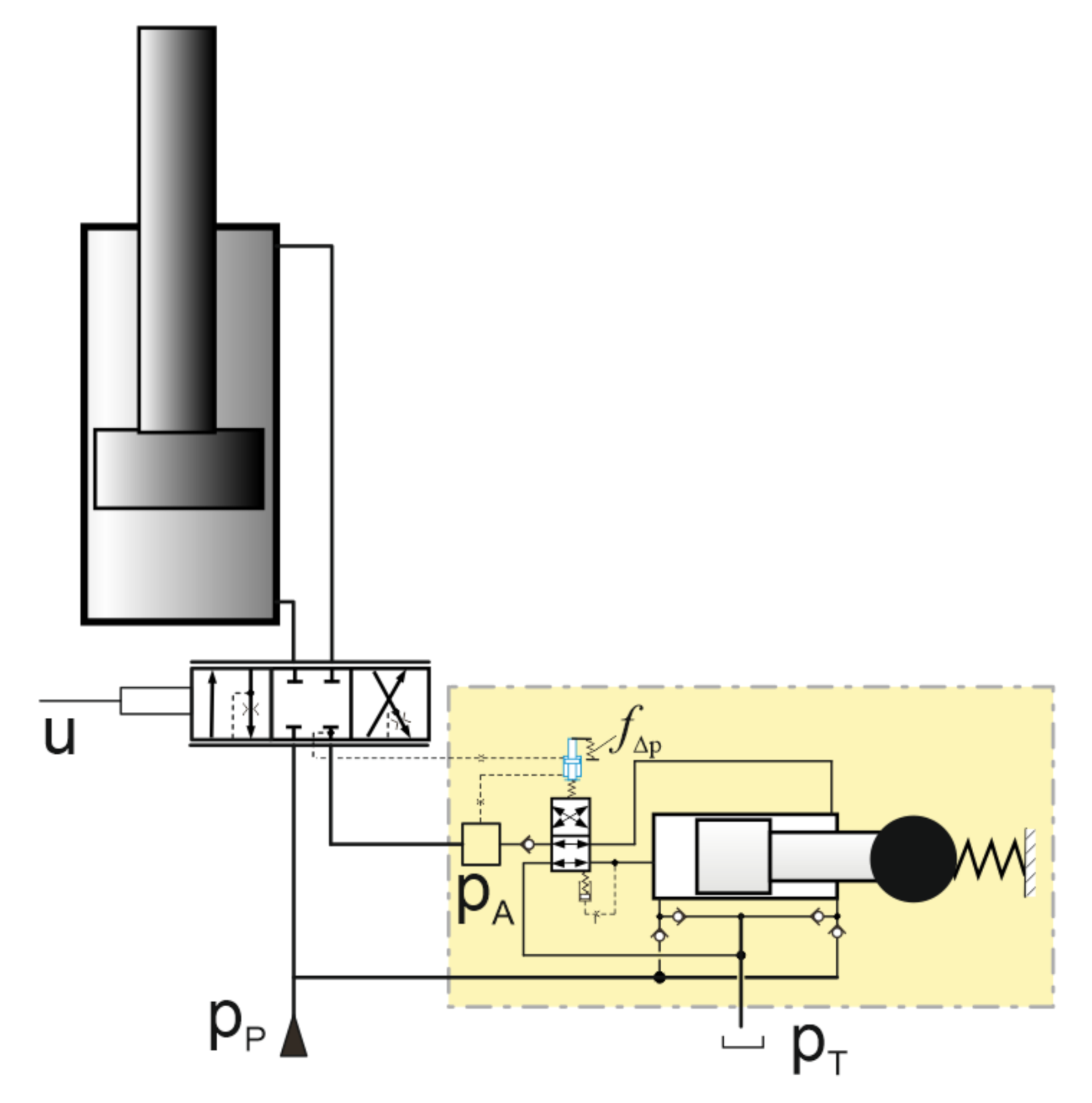
3.1. Concept
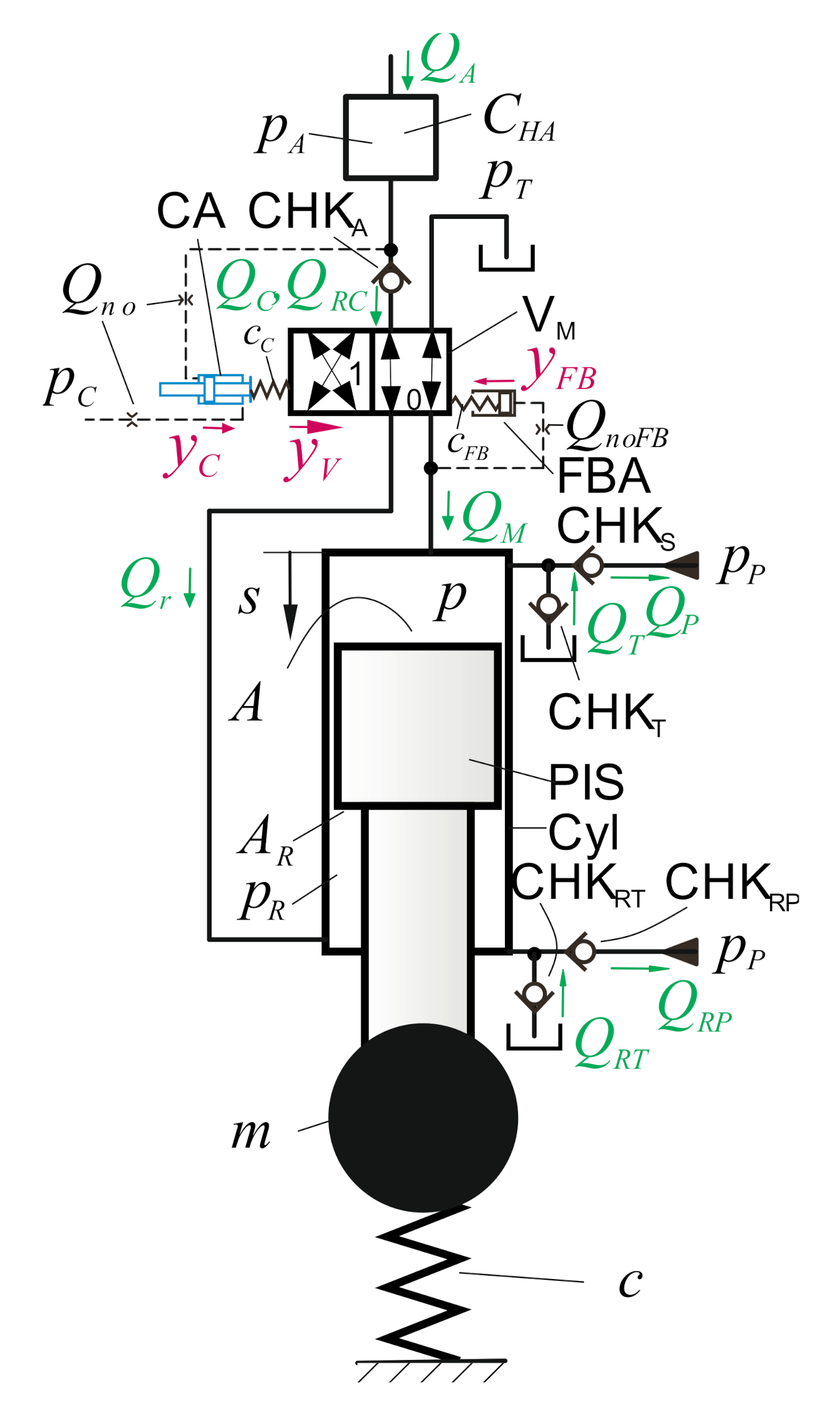
The proposed circuitry is shown in
Figure 6. A double stroke cylinder with piston (PIS) and rod sided areas
A and
AR forms a hydraulically actuated oscillator with the attached mass
m and the spring with constant
c. The main valve V
M is of the 4-2 way type and is actuated by the control actuator (CA) and feedback actuator (FBA). The system realizes a pressure relief function for the pressure
pA in the hydraulic capacitance
CHA. The disturbance of the system is the flow
QA and the desired value of
pA is set by the pressure
pC. The system constitutes a step-up converter to regain part of the hydraulic power
pA.QA.
The working principle is that CA switches VM into state 1 if pA > pC which makes the oscillator, performing a half oscillation (A-phase) followed by a first backward motion (P-phase) feeding, part of the received energy to the system pressure line via the valve CHKS. Then, driven by the feedback actuator FBA, the valve switches back to state 0, allowing the spring to retract the piston until it stops. If the spring force in this uppermost position is sufficiently negative, part of its strain energy is fed to the system pressure line by CHKRP. The oscillator stops there if CA does not provoke the next oscillation. The two tank sided check valves CHKT and CHKRT avoid cavitation on both cylinder chambers.
A key element of the functioning principle is FBA. It comprises a plunger pushing on the valve by a spring (constant cFB). It is activated by pressure p in the main cylinder chamber. Oscillation of p brings in the driving impulse with the right timing for the motion yV of the main valve VM. The spring cFB acts as a hydraulic capacitance element in combination with the plunger (area AFB) and the orifice QNoFB (nominal flow rate) which creates a delay of the feedback force relative to pressure p. In addition, and in combination with cC, it serves as the oscillator spring for the valve spool, which has mass mV. The two orifices QNo in the lines to the CA give this actuator’s force a delayed response to its input pressures.
The rod side chamber (AR) keeps the oscillator at the final position after a full operation cycle to keep a defined state until the next cycle is carried out. This also avoids the loss of the spring potential energy in this state by damped oscillations which would occur otherwise.
3.2. Simulation Model
This system’s working principle does not lend itself to an evaluation by a simple model with analytical solutions. Therefore, a moderately complex dynamical model is formulated leading to a set of nonlinear ordinary differential equations which are solved by numerical integration. The model comprises the following relations: an equation of motion of the oscillator and the valve spool with the pressure forces of both cylinder chambers, a viscous type damping of the piston motion, contact (
FC, FVC) and valve actuator forces (
FAC, FFB):
Pressure buildup equations for
p, pR, pA:
Evolution equations for the actuator positions
yC and
yFB. The inertia forces of the tiny moving elements are neglected, since the motion speed is controlled by the orifices. Therefore, the two Equation (12) represent the equilibrium conditions made explicit w.r.t. the actuator piston speeds
:
The forces and flow rates in Equations (10)–(12) are related to the state vector (
T is the transpose)
by the following spring force equations:
Contact forces at the end stop the positions of both actuator pistons, based on elastic and damping forces. The latter act only at the landing and not at the lift-off.
Flow rates by the orifice equation:
The special functions
orifice, sg, and sg1:
The model does not include check valve dynamics and flow forces in the valve equation of motion. Both effects depend strongly on the specific design of the valves. Since this is a basic study without information about the details of component selection, these dynamic effects are neglected.
3.3. System Parameters
Unfortunately, a compact model of the system is missing. Therefore, only a few rules from the behavior of the OMC of
Section 2 are available. The oscillator operates around its resonance frequency
ω. This frequency has to be handled by the other components as well, and in particular by all the valves, hence is selected from knowledge about the feasible frequencies in hydraulic switching control. This frequency and a typical oscillation amplitude determine the oscillation speed and, together with the piston area, also the size of the flow rate. From the oscillator flow rates, the valve nominal flow rates can be estimated. The natural frequency of the valve spool, determined by its mass
mV and the spring constants
cC and
cFB, must be in the order of the operating frequency. The orifices’ sizes have been found by trial and error.
The damping coefficient
d of the oscillator was determined from the viscous shear force between a centered piston and cylinder, bore with diameter
dK, length
lK, fluid viscosity
μ and sealing gap
hg by the following equation:
The contact damping coefficients dC and dCV have been selected to provide critical damping in order to prevent bouncing when the oscillator or valve reach end stop positions.
The selected parameters are given in
Table 1, where applicable, by dimensioning rules.
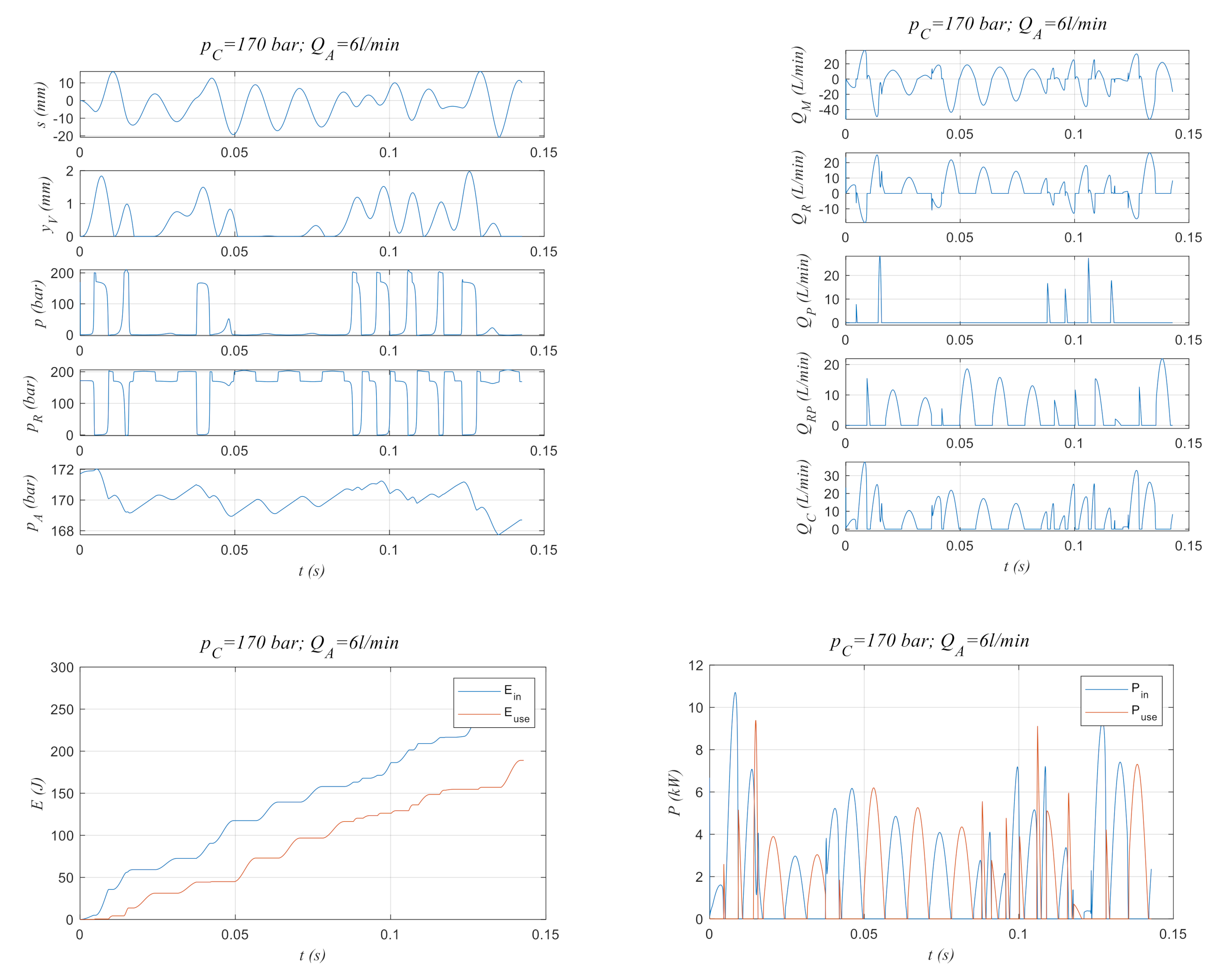
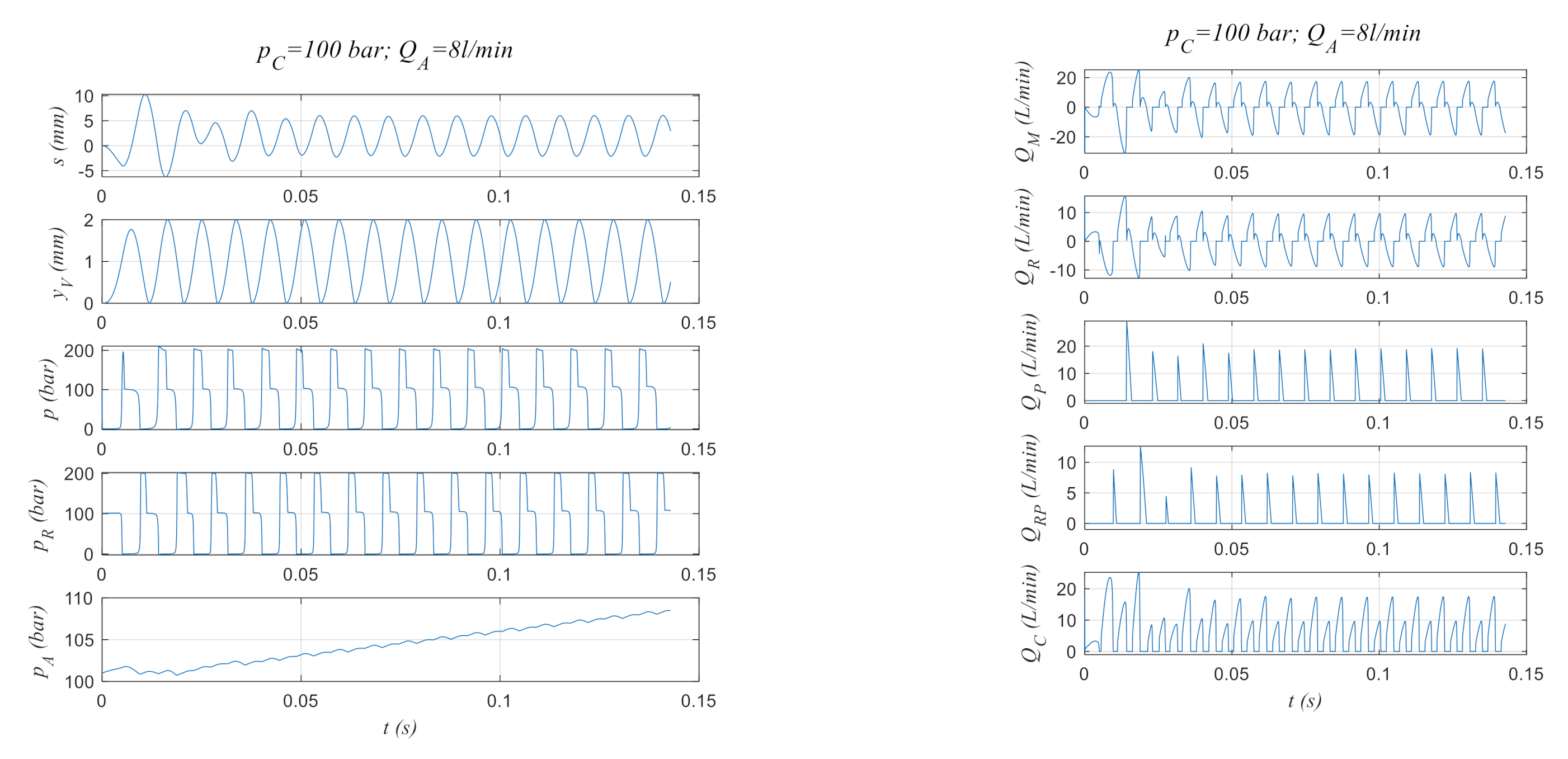
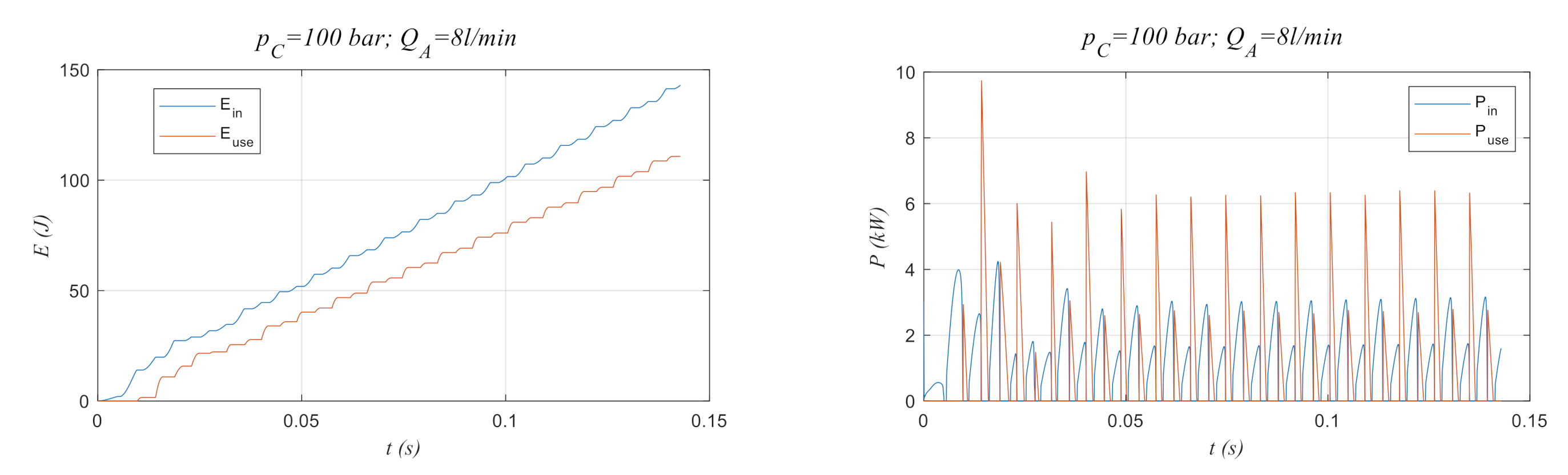
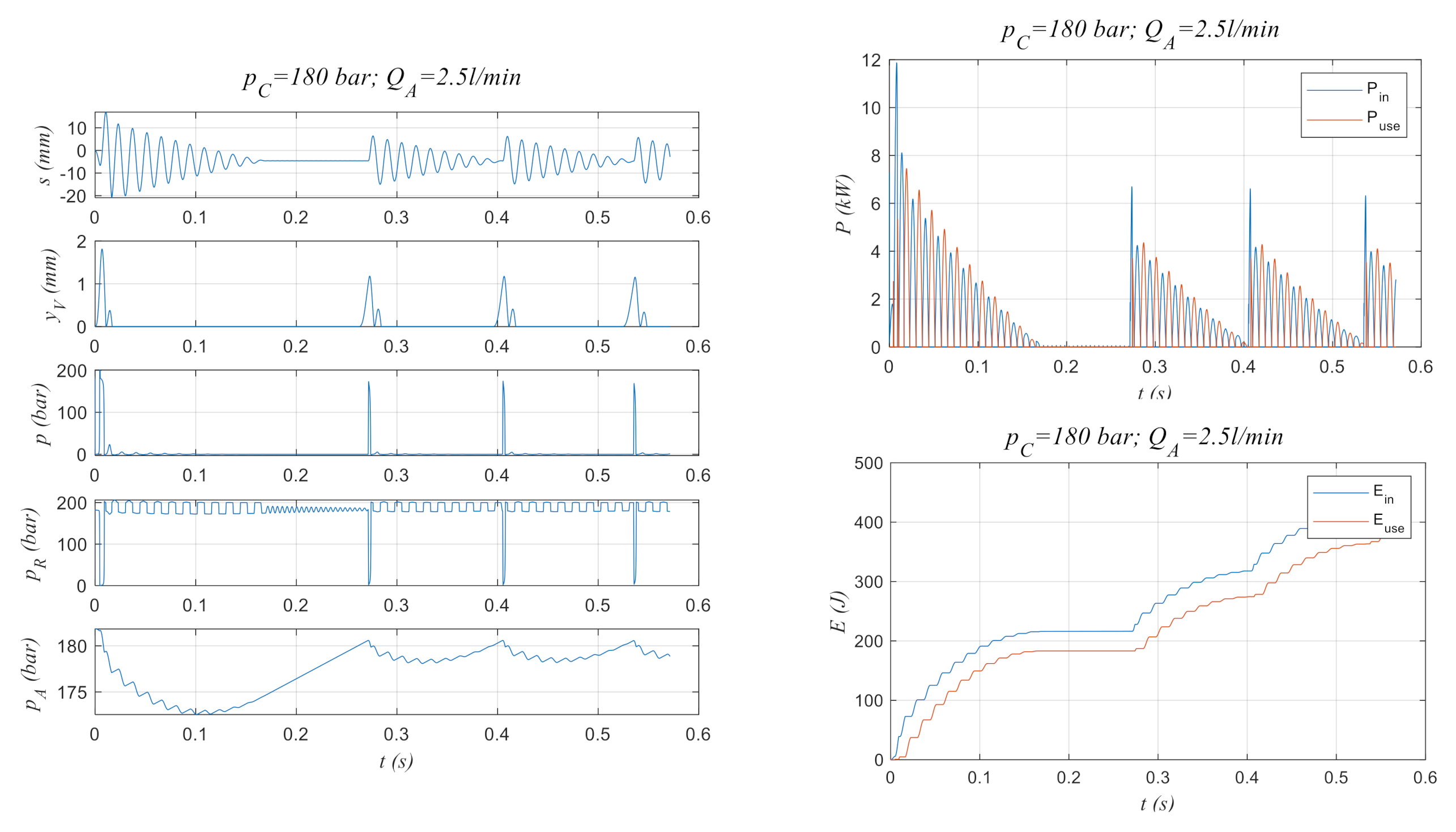
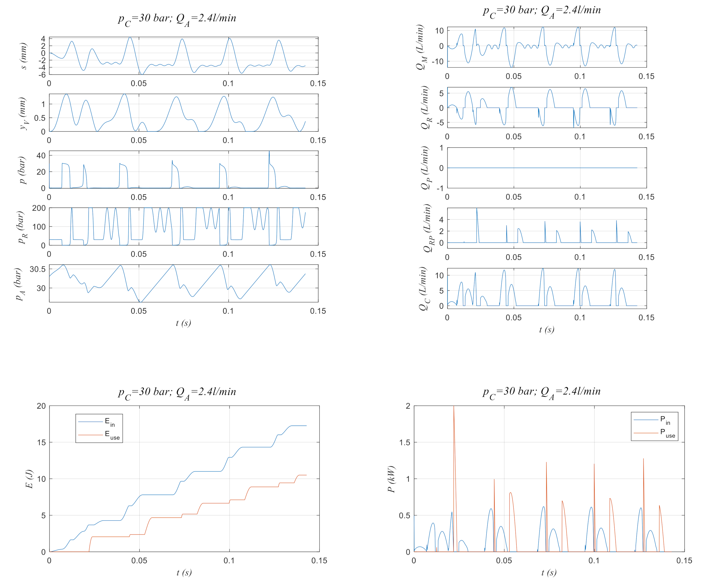
3.5. Simulation Results
The diagrams in
Figure 7,
Figure 8 and
Figure 9 show five of the seven states, the most significant flow rates, and the input and recuperated energies and powers, respectively, for three operation conditions.
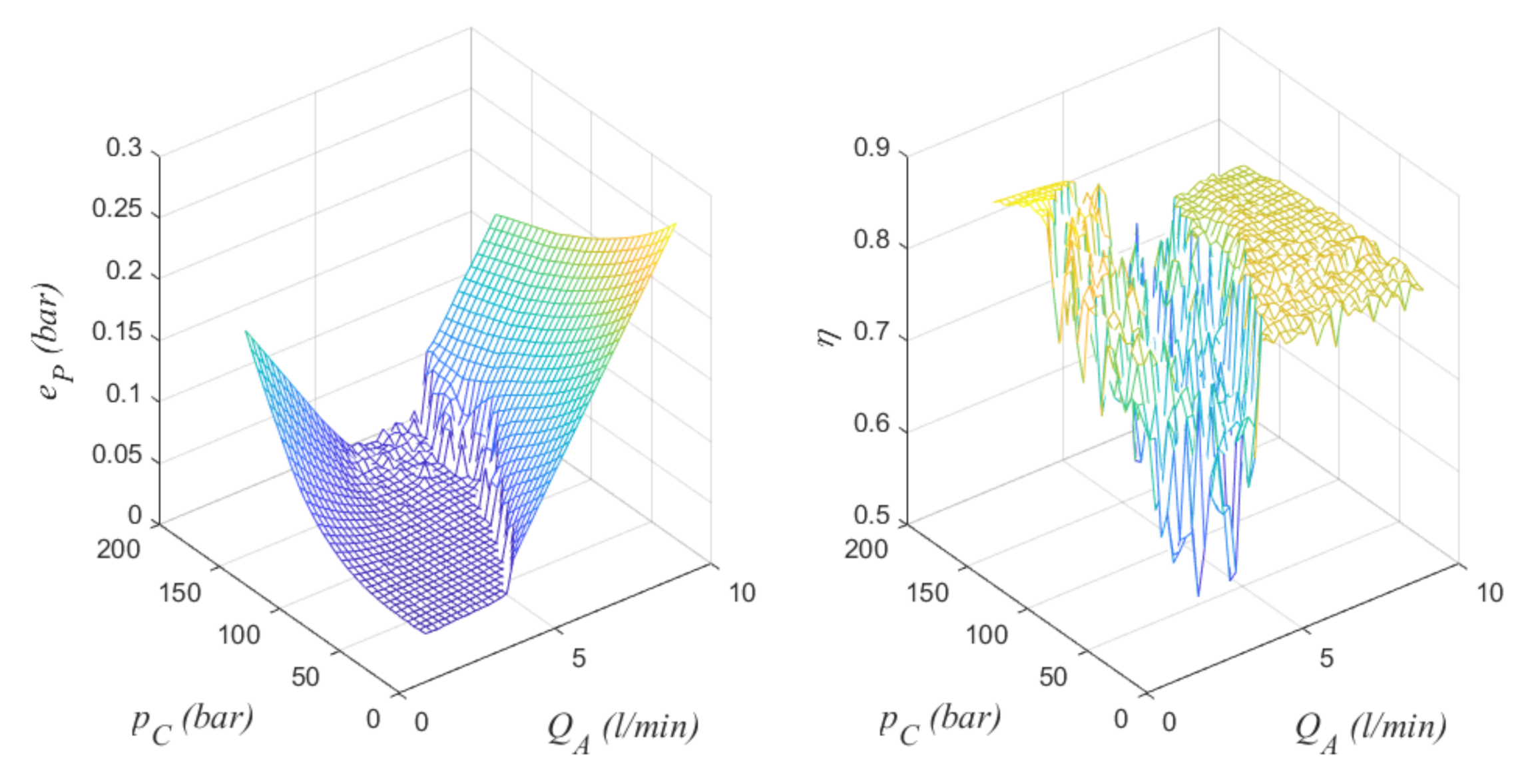
Figure 10 gives the performance values for a product set of 31
pC and 41
QA values. The low flow rate and low-pressure case of
Figure 7 shows a moderate oscillation amplitude and effective oscillations occurring with only half of the nominal frequency of 70 hertz.
The system quasi pauses for one nominal period to get sufficient energy for a strong enough oscillation from the slowly incoming hydraulic energy. The input capacitance
CHA presumably plays a significant role for that.
pA varies between 29.7 and 30.6 bar, and the error norm is
eP = 0.0067 bar. Recuperation happens only from the rod side chamber, as the plots of pressures
p,
pR and flow rates
QP,
QRP show. The operation condition with the high pressure and flow rate of
Figure 8 leads to higher oscillation amplitudes and clustered oscillations separated by phases with poor oscillation. Pressure control is still achieved with peak values of 168 and 172 bar, which corresponds to
eP = 0.0188 bar. Recuperation is dominated by the rod side chamber, but some portion is contributed by the main chamber, too. The nature of the dynamical system response is not obvious from the plot, but it is not periodic or subharmonic.
The system cannot control a flow rate of 8 L/min for p
C = 100 bar, according to the results in
Figure 9. The converter’s throughput is insufficient, and the
pC increases steadily. The recuperation efficiency is 0.77 and both chambers recuperate. The graph of
eP shows small values for ranges where the η graph is strongly scattered. The reason for this apparent coincidence is not clear and lies in the complex dynamical properties of this converter. The error
eP is also large for small flow rates and high pressures. This stems for the inability of the converter to master the small flow rates in a steady manner, as
Figure 11 demonstrates. In the diagrams of
Figure 10, only 10 nominal periods are simulated when the converter performs decaying oscillations which consume more flow rate then is inputted by
QA. There, the pressure
pA falls first and increases afterwards. A kind of subharmonic steady-state oscillatory response emerges with ten times the nominal period. Thus, the performance is fully different from the high flow rate area, where the converter cannot master the high flow rate at all, and the pressure increases permanently until it reaches
pP and one of the check valves CHK
S or CHK
A allows a flow to the system line.
4. Comparison with Other Switching Converters and Potential Applications
In the following, the pros and cons of other main hydraulic switching converters compared to the studied OMC, and partly among one other, are stated.
Buck converter (inertance tube) with fast solenoid switching valve(s): Features a simpler concept and allows a good control performance in combination with advanced controllers. Fast switching valves, required to reduce length of inertance tube and size of pulsation attenuation and accumulator, are not available on the market. The length of the inertance tube may be an impediment for some applications. Elevated tank pressure is required to avoid cavitation.
However, if the configuration is modified to operate as a step-up converter, the latter problem is avoided. Furthermore, hydraulic methods for switching control are basically also applicable to inertance tube converters, as the hydraulic ram demonstrates.
A switching converter with a displacement machine and a flywheel as the inertance element: It is a simple concept. The free adjustment of inertance via the flywheel moment of inertia allows an operation with lower switching frequencies feasible with off-the-shelf valves, but reduces control bandwidth. The cost of displacement machines and friction and uneven behavior at low flow rates are further disadvantages.
Oscillating piston converter with fast solenoid switching valves: The switching events can be optimized w.r.t efficiency or control bandwidth. The total construction size is smaller than with an inertance converter tube if operated with comparable switching frequencies. However, off-the-shelf valves for a practically convincing realization are missing.
The comparisons above are mixing two main functional elements of switching converters: (i) the switches (switching valves) and the (ii) inertance element. The third functional element, the pressure and flow ripples attenuation device, is not addressed. In this study, it is given by the capacitance CHA on the input side, while the constant pressure ports for system and tank pressure on the output side are assumed to provide means for coping with pulsating flows. In addition to the switching frequency, the unevenness of the flow generated by the converter has a strong influence on the size of the attenuation device, e.g., on the volume of an accumulator. A solid answer as to how the different converter principles compare in this respect needs a detailed analysis, which has no place in this paper. In the presented OMC, the control is also involved, whereas in systems with electrically actuated valves, the control is done separately, typically by some control software.
The presented OMC is configured as a pressure limiting device with recuperation capability. It “costs” more than a pressure relief valve, not only in terms of investment costs but also in terms of space, weight, noise, potential hydraulic disturbances of the overall system, and risk of failure. It can only pay if the energetic losses saved over-compensate these costs. Furthermore, its control performance in terms of precision and response dynamics is limited.
Generally speaking, its potential applications are seen where energy is still wasted but savings are relevant, control performance requirements are moderate, and a cost-effective solution is required. Costs are a matter of sold units and whether standard components can be used. In many technical systems, using fluid power drives the changeover to a really new concept, particularly if theis needs new components, is hard to make. However, if the main concept may be preserved and only an additional device needs to be added and provides clear benefits, the chance of a practical realization is bigger.
A potential case of such use is briefly sketched here: meter out control of a cylinder drive according to the schematic in
Figure 12. A proportional valve provides the directional and speed control functions, as in a load sensing system. The compensation valve of a load sensing system is replaced by the converter which uses the pressure difference
Δp at the load sensing meter out as the control input and tries to keep this value constant. The pressure difference can be adjusted by a spring force
fΔp. Thus, the speed of the cylinder is proportional to valve input
u. The control performance requirements in typical load sensing applications are moderate and are primarily determined by the proportional valve. The energy lost by the compensation valve can be saved.
Useful application in other domains, such as renewable energies, depends on the size of the system. For large units handling powers in the hundreds of kilowatts range or beyond, the wins by using precise control probably overcome the costs of electrically actuated valves. If the costs of other sub-systems, such as the structural parts, are high, the very efficient transfer of energy to the net is a necessity for an economically feasible implementation. If, however, the prime energy is abound and the hydraulic system costs are high, the presented OMC or modification of it may be useful.
5. Summary and Outlook to Further Work
The presented concept of an oscillating mass converter with hydraulic control seems to have the intended properties if applied for step-up conversion: provide reasonable control and the ability to recuperate energy. The computed efficiencies are well above 50% in a large operation range and the control error is relatively small. The system constitutes a coupled nonlinear oscillation system which features a complex response behavior which is not currently fully understood and constitutes an interesting and theoretically challenging problem. The use for a kind of load sensing meter out control was sketched.
The system parameters for the simulation study have been selected partly on the basis of simple design rules, determined partly by trial and error. The system deserves design optimization, for instance by applying genetic algorithms. This is one of the next research steps.
It is very likely that modifications of the presented solution offer performance gains. One way to go is the use of slow, semi-active electric control for better adjustment of the system to different operating conditions.
The used model does not include some effects which will influence the performance: response dynamics of the check valves, friction and flow forces in the main valve, and sealing friction of the cylinder, in case seals are applied at the piston or rod. General problems of hydraulic switching control are pulsations and mechanical shake. A potential way to reduce these problems is the phase shifted operation of more than one converter in a parallel arrangement, as studied in [
22] for the buck converter. Proper phase shifting is simple for electric valve control but non-trivial for hydraulic control. The interaction of several such converters is an interesting problem, deserving of a scientific investigation.
The hydraulic control of switching converters is not limited to the oscillating mass converter but can be applied to other concepts as well. The author is currently working on the hydraulic control of the buck (step down) converter with an inertance tube. The expected advantages are cost saving, component availability, and in this case, the realization of higher switching frequencies, since hydraulic actuation is more powerful than magnetic actuation.
Last but not least, the practical success of any of such hydraulically controlled switching converters depends on a felicitous embodiment design.


