The Evaluation of the Corrosion Rates of Alloys Applied to the Heating Tower Heat Pump (HTHP) by Machine Learning
Abstract
1. Introduction
2. Models
2.1. Support Vector Machine
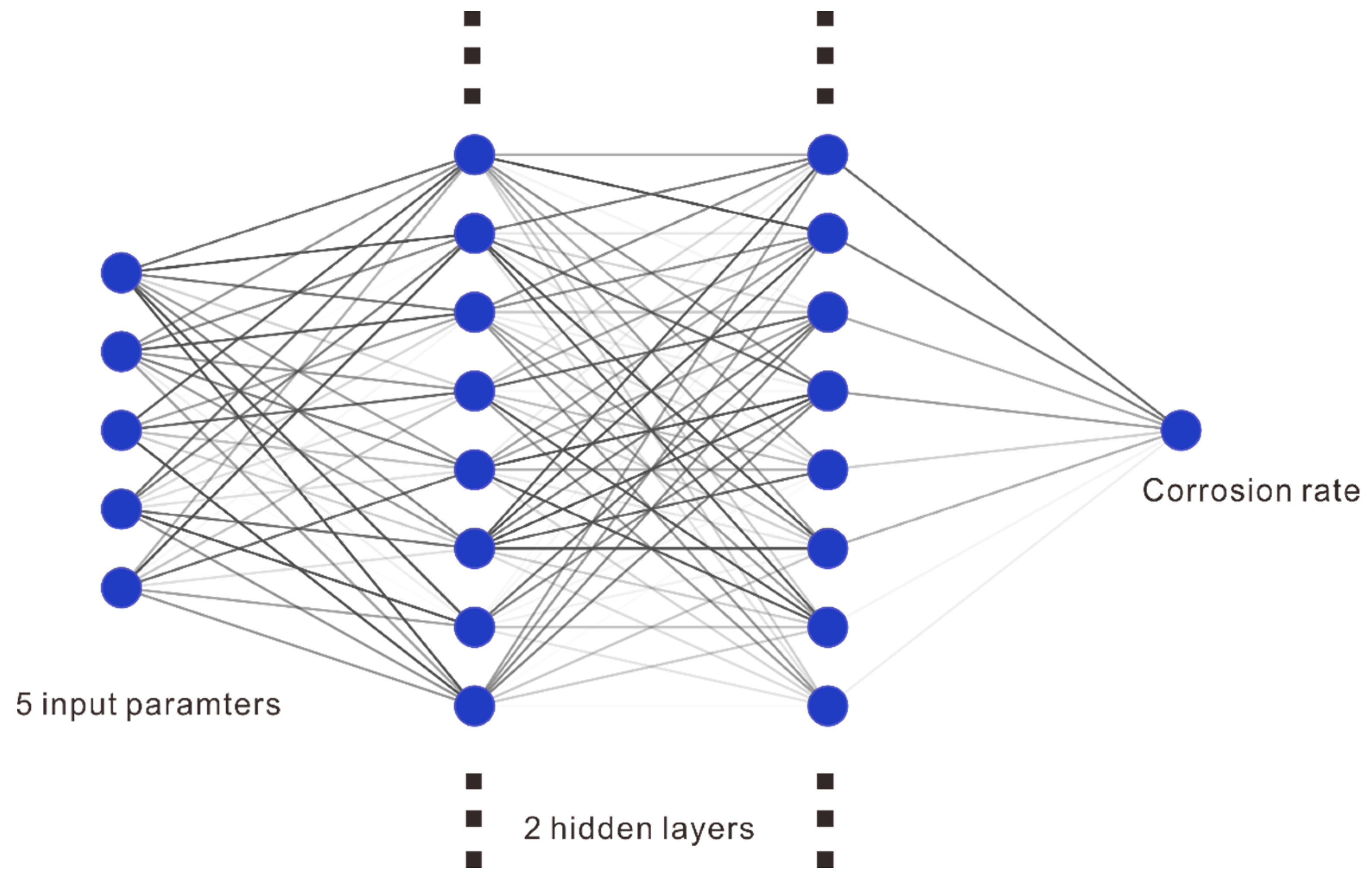
2.2. Artificial Neural Network
3. Results and Discussion
4. Conclusions
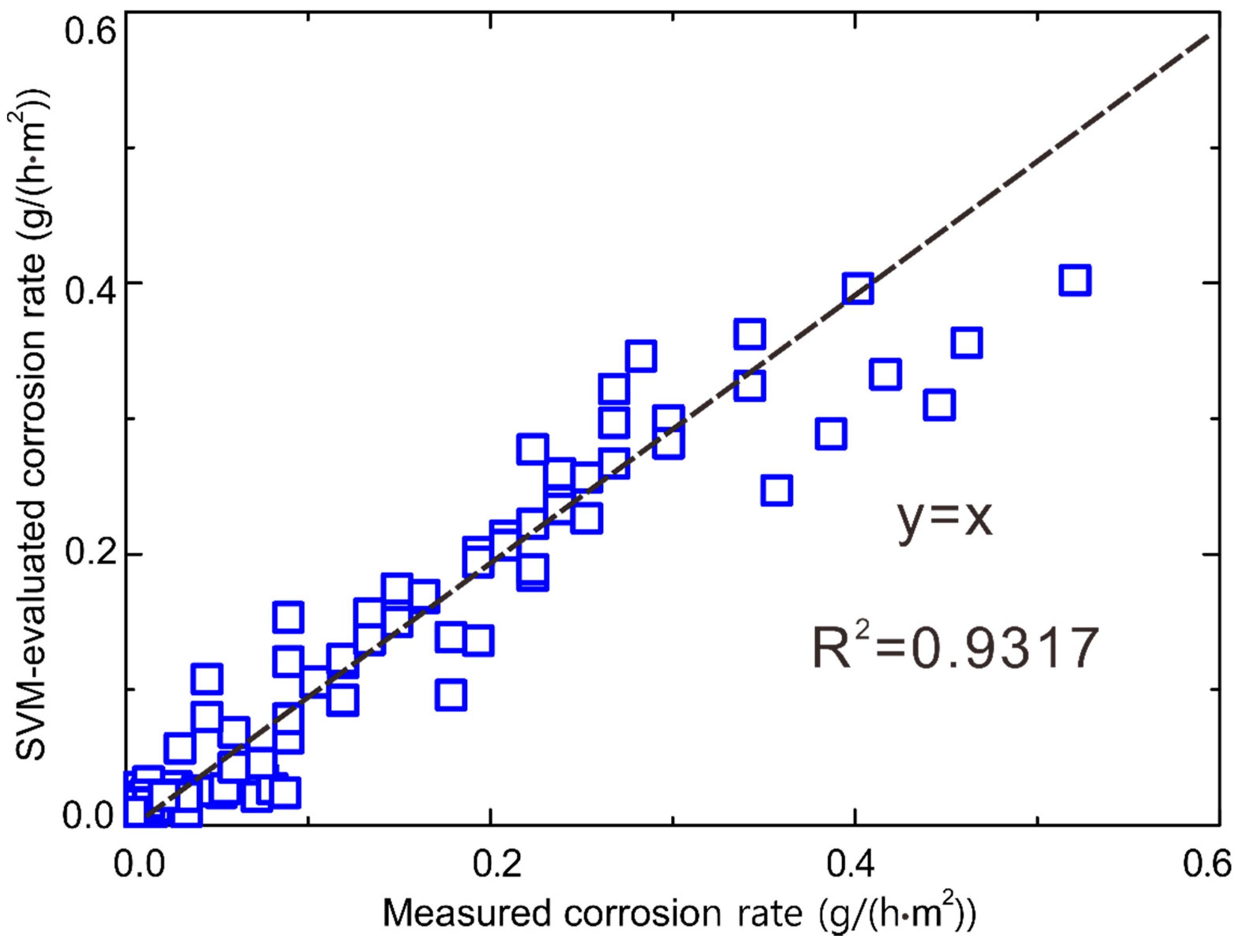
- The SVM can be used to obtain a reasonable corrosion rate, the R2 value being 0.9317.
- The MSE of the training dataset for the ANN decreases with the epoch and can be convergent. Meanwhile, there is a local minimum region broken by the presently used optimizer RMSProp for the MSE of the validation dataset. It can be concluded that after around 60,000 epoch, the obtained ANN model can achieve the best performance.
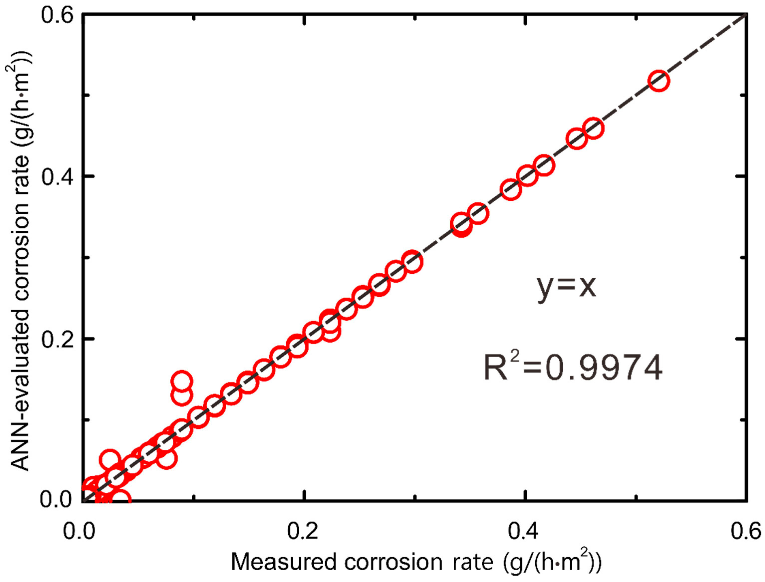
- The good agreement between the ANN-evaluated corrosion rate and the measured ones indicates that the presently obtained ANN model is of better accuracy and reliability since the R2 value is 0.9974. The present work can contribute to the prediction of the corrosion rates of copper H65, aluminum 3003, and 20# steel without any prior experiments, thus improving the performance and service life of the HTHP.
Author Contributions
Funding
Institutional Review Board Statement
Informed Consent Statement
Data Availability Statement
Acknowledgments
Conflicts of Interest
References
- Building Energy Research Center of Tsinghua University. 2020 Annual Report on China Building Energy Efficiency; China Architecture & Building Press: Beijing, China, 2020; pp. 2–10. [Google Scholar]
- Cui, H.; Li, N.; Wang, X.; Peng, J.; Li, Y.; Wu, Z. Optimization of reversibly used cooling tower with downward spraying. Energy 2017, 127, 30–43. [Google Scholar] [CrossRef]
- Niksiar, A.; Rahimi, A. Energy and exergy analysis for cocurrent gas spray cooling systems based on the results of mathematical modeling and simulation. Energy 2009, 34, 14–21. [Google Scholar] [CrossRef]
- Song, P.; Xiao, H.; Shi, W.; Li, X.; Wang, B.; Li, Z.; Zhang, Y.; Zhong, H. Experimental investigation on closed-type heating tower using glycerol solution. Int. J. Refrig. 2019, 99, 272–287. [Google Scholar] [CrossRef]
- Cui, H.; Li, N.; Peng, J.; Cheng, J.; Li, S. Study on the dynamic and thermal performances of a reversibly used cooling tower with upward spraying. Energy 2016, 96, 268–277. [Google Scholar] [CrossRef]
- Cui, H.; Li, N.; Peng, J.; Cheng, J.; Zhang, N.; Wu, Z. Modeling the particle scavenging and thermal efficiencies of a heat absorbing scrubber. Build Environ. 2017, 111, 218–227. [Google Scholar] [CrossRef]
- Liu, J.; Sun, Y.; Wang, W.; Zhu, J. Performance evaluation of air source heat pump under unnecessary defrosting phenomena for nine typical cities in China. Int. J. Refrig. 2017, 74, 385–398. [Google Scholar] [CrossRef]
- Liang, C.; Wen, X.; Liu, C.; Zhang, X. Performance analysis and experimental study of heat-source tower solution regeneration. Energ Convers Manag. 2014, 85, 596–602. [Google Scholar] [CrossRef]
- Huang, S. Study on Optimization and Evaluation of Heating Tower Heat Pump System. Ph.D. Thesis, Southeast University, Nanjing, China, 2019. [Google Scholar]
- Su, Z. Performance Analysis of Wet Heat Source Tower Heat Pump System under Winter Condition in North China. Master’s Thesis, Tianjin University, Tianjin, China, 2010. [Google Scholar]
- Lv, Z.; Liang, C.; Huang, S.; Zhang, X. Heat and mass transfer performance of porous corrugated packing in heat-source tower. J. Cent. South Univ. 2018, 49, 1003–1010. [Google Scholar]
- Feng, Q.; Yan, B.; Chen, P.; Shirazi, S. Failure analysis and simulation model of pinhole corrosion of the refined oil pipeline. Eng. Fail. Anal. 2019, 106, 104177. [Google Scholar] [CrossRef]
- Benea, L.; Simionescu, N.; Mardare, L. The effect of polymeric protective layers and the immersion time on the corrosion behavior of naval steel in natural seawater. J. Mater. Res. Technol. 2020, 9, 13174–13184. [Google Scholar] [CrossRef]
- Faisal, D.; Ryan, W.; Vijay, S.; Mahroo, E.; Steve, M. Predicting Corrosion rate in Chilled HVAC Pipe Network: Coupon vs Linear Polarisation Resistance method. Eng. Fail. Anal. 2020, 109, 104261. [Google Scholar]
- Ma, L.; Wang, J.; Zhang, D.; Huang, Y.; Huang, L.; Wang, P.; Qian, H.; Li, X.; Terryn, H.A.; Mole, J.M.C. Dual-action self-healing protective coatings with photothermal responsive corrosion inhibitor nanocontainers. Chem. Eng. J. 2021, 404, 127118. [Google Scholar] [CrossRef]
- Tan, B.; Xiang, B.; Zhang, S.; Qiang, Y.; Xu, L.; Chen, S.; He, J. Papaya leaves extract as a novel eco-friendly corrosion inhibitor for cu in H2SO4 medium. J Colloid Interf. Sci. 2021, 582, 918–931. [Google Scholar] [CrossRef] [PubMed]
- Duan, T.; Peng, W.; Ding, K.; Guo, W.; Hou, J.; Cheng, W.; Liu, S.; Xu, L. Long-term field exposure corrosion behavior investigation of 316L stainless steel in the deep sea environment. Ocean Eng. 2019, 189, 06405. [Google Scholar] [CrossRef]
- Zhang, P. Experimental Research on Metal Corrosion Performance of Coolants on Cold and Heat Source Side in Heat Source Tower Heat Pump. Ph.D. Thesis, Hunan University, Changsha, China, 2019. [Google Scholar]
- Kumari, S.; Tiyyagura, H.R.; Douglas, T.L.; Mohammed, E.A.; Adriaens, A.; Fuchs-Godec, R.; Mohan, M.K.; Skirtach, A.G. ANN prediction of corrosion behaviour of uncoated and biopolymers coated cp-Titanium substrates. Mater Des. 2018, 157, 35–51. [Google Scholar] [CrossRef]
- Smuga-Kogut, M.; Kogut, T.; Markiewicz, R.; Słowik, A. Use of Machine Learning Methods for Predicting Amount of Bioethanol Obtained from Lignocellulosic Biomass with the Use of Ionic Liquids for Pretreatment. Energies 2021, 14, 243. [Google Scholar] [CrossRef]
- Wu, J.; Zhang, G.; Zhang, Q.; Zhou, J.; Wang, Y. Artificial neural network analysis of the performance characteristics of a reversibly used cooling tower under cross flow conditions for heat pump heating system in winter. Energ. Build. 2011, 43, 1685–1693. [Google Scholar] [CrossRef]
- Alimoradi, H.; Soltani, M.; Shahali, P.; Moradi Kashkooli, F.; Larizadeh, R.; Raahemifar, K.; Adibi, M.; Ghasemi, B. Experimental Investigation on Improvement of Wet Cooling Tower Efficiency with Diverse Packing Compaction Using ANN-PSO Algorithm. Energies 2021, 14, 167. [Google Scholar] [CrossRef]
- Awad, M.; Khanna, R. Efficient Learning Machines; Apress: New York, NY, USA, 2015. [Google Scholar]
- Quinonero-Candela, J.Q.; Rasmussen, C.E. A unifying view of sparse approximate Gaussian process regression. J. Mach. Learn. Res. 2005, 6, 1939–1959. [Google Scholar]
- Yin, C.; Goudriaan, J.; Lantinga, E.A.; Vos, J.; Spiertz, H.J. A Flexible Sigmoid Function of Determinate Growth. Ann. Bot 2003, 91, 361–371. [Google Scholar] [CrossRef]
- Wanto, A.; Windarto, A.P.; Hartama, D.; Parlina, I. Use of Binary Sigmoid Function And Linear Identity In Artificial Neural Networks For Forecasting Population Density. J. Inf. Technol. 2017, 1, 43–54. [Google Scholar] [CrossRef]
- Han, J.; Moraga, C. The Influence of the Sigmoid Function Parameters on the Speed of Backpropagation Learning. Lect. Notes Comput. Sci. 1995, 930, 195–201. [Google Scholar]
- Zou, F.; Shen, L.; Jie, Z.; Zhang, W.; Liu, W. A Sufficient Condition for Convergences of Adam and RMSProp. In Proceedings of the IEEE/CVF Conference on Computer Vision and Pattern Recognition (CVPR), Long Beach, CA, USA, 16–20 June 2019; pp. 11127–11135. [Google Scholar]
- Tieleman, T.; Hinton, G. RMSProp, COURSERA: Lecture 6.5-Neural Networks for Machine Learning. 2012. Available online: https://www.coursera.org/.
- Wiens, T.S.; Dale, B.C.; Boyce, M.S.; Kershaw, G.P. Three way k-fold cross-validation of resource selection functions. Ecol. Model 2008, 212, 244–255. [Google Scholar] [CrossRef]
- Bengio, Y.; Grandvalet, Y. No unbiased estimator of the variance of k-fold cross-validation. J. Mach. Learn. Res. 2004, 5, 1089–1105. [Google Scholar]
- Rodriguez, J.D.; Perez, A.; Lozano, J.A. Sensitivity analysis of k-fold cross validation in prediction error estimation. IEEE Trans. Pattern Anal. Mach. Intell. 2009, 32, 569–575. [Google Scholar] [CrossRef]
- Fushiki, T. Estimation of prediction error by using K-fold cross-validation. Stat. Comput. 2011, 21, 137–146. [Google Scholar] [CrossRef]
- Wong, T.T. Performance evaluation of classification algorithms by k-fold and leave-one-out cross vali-dation. Pattern Recogn. 2015, 48, 2839–2846. [Google Scholar] [CrossRef]



| Alloy | Coolant | Corrosion Time (Days) | Flow Velocity (m/s) | Temperature (°C) | Corrosion Rate (g/(h·m2)) | |||
|---|---|---|---|---|---|---|---|---|
| Measured | Uncertainty% | SVR-Evaluated | ANN-Evaluated | |||||
| Copper H65 | BF2354 | 30 | 0 | 15 | 0.07528 | 0.08 | 0.03276 | 0.05264 |
| Aluminum 3003 | BF2354 | 30 | 0 | 15 | 0.00805 | 0.74 | 0.01409 | 0.00796 |
| 20# Steel | BF2354 | 30 | 0 | 15 | 0.06005 | 0.10 | 0.03538 | 0.05975 |
| Copper H65 | HG3500 | 30 | 0 | 15 | 0.00259 | 2.31 | 0.01510 | 0.00260 |
| Aluminum 3003 | HG3500 | 30 | 0 | 15 | 0.00201 | 2.98 | 0.00443 | 0.00218 |
| 20# Steel | HG3500 | 30 | 0 | 15 | 0.01580 | 0.38 | 0.02249 | 0.01563 |
| Copper H65 | BK3000 | 30 | 0 | 15 | 0.00862 | 0.69 | 0.02358 | 0.00925 |
| Aluminum 3003 | BK3000 | 30 | 0 | 15 | 0.00575 | 1.04 | 0.00819 | 0.00550 |
| 20# Steel | BK3000 | 30 | 0 | 15 | 0.00201 | 2.98 | 0.02818 | 0.00222 |
| Copper H65 | BL3500 | 30 | 0 | 15 | 0.00517 | 1.16 | 0.01763 | 0.00548 |
| Aluminum 3003 | BL3500 | 30 | 0 | 15 | 0.00374 | 1.60 | 0.00494 | 0.00393 |
| 20# Steel | BL3500 | 30 | 0 | 15 | 0.05229 | 0.11 | 0.02384 | 0.05274 |
| Copper H65 | YH6830 | 30 | 0 | 15 | 0.00287 | 2.09 | 0.01605 | 0.00295 |
| Aluminum 3003 | YH6830 | 30 | 0 | 15 | 0.00575 | 1.04 | 0.00663 | 0.00580 |
| 20# Steel | YH6830 | 30 | 0 | 15 | 0.01207 | 0.50 | 0.02415 | 0.01209 |
| Copper H65 | ZP3682 | 30 | 0 | 15 | 0.01868 | 0.32 | 0.02035 | 0.01947 |
| Aluminum 3003 | ZP3682 | 30 | 0 | 15 | 0.01034 | 0.58 | 0.01143 | 0.01014 |
| 20# Steel | ZP3682 | 30 | 0 | 15 | 0.06723 | 0.09 | 0.02869 | 0.06643 |
| Copper H65 | BF2354 | 30 | 0 | 10 | 0.02772 | 0.22 | 0.02878 | 0.02764 |
| Aluminum 3003 | BF2354 | 30 | 0 | 10 | 0.01076 | 0.56 | 0.01184 | 0.01052 |
| 20# Steel | BF2354 | 30 | 0 | 10 | 0.01265 | 0.47 | 0.03227 | 0.01239 |
| Copper H65 | HG3500 | 30 | 0 | 10 | 0.02045 | 0.29 | 0.01204 | 0.02026 |
| Aluminum 3003 | HG3500 | 30 | 0 | 10 | 0.00457 | 1.31 | 0.00294 | 0.00468 |
| 20# Steel | HG3500 | 30 | 0 | 10 | 0.02422 | 0.25 | 0.02024 | 0.05067 |
| Copper H65 | BK3000 | 30 | 0 | 10 | 0.01884 | 0.32 | 0.01989 | 0.01836 |
| Aluminum 3003 | BK3000 | 30 | 0 | 10 | 0.01319 | 0.45 | 0.00621 | 0.00446 |
| 20# Steel | BK3000 | 30 | 0 | 10 | 0.03929 | 0.15 | 0.02535 | 0.03791 |
| Copper H65 | BL3500 | 30 | 0 | 10 | 0.02018 | 0.30 | 0.01424 | 0.01953 |
| Aluminum 3003 | BL3500 | 30 | 0 | 10 | 0.00431 | 1.39 | 0.00321 | 0.00407 |
| 20# Steel | BL3500 | 30 | 0 | 10 | 0.07185 | 0.08 | 0.02130 | 0.07100 |
| Copper H65 | YH6830 | 30 | 0 | 10 | 0.00942 | 0.64 | 0.01330 | 0.00970 |
| Aluminum 3003 | YH6830 | 30 | 0 | 10 | 0.00807 | 0.74 | 0.00537 | 0.00810 |
| 20# Steel | YH6830 | 30 | 0 | 10 | 0.03337 | 0.18 | 0.02217 | 0.03379 |
| Copper H65 | ZP3682 | 30 | 0 | 10 | 0.03041 | 0.20 | 0.01791 | 0.03052 |
| Aluminum 3003 | ZP3682 | 30 | 0 | 10 | 0.00269 | 2.23 | 0.01036 | 0.00289 |
| 20# Steel | ZP3682 | 30 | 0 | 10 | 0.05463 | 0.11 | 0.02696 | 0.05413 |
| Copper H65 | BF2354 | 30 | 0 | 0 | 0.03144 | 0.19 | 0.02149 | 0.03034 |
| Aluminum 3003 | BF2354 | 30 | 0 | 0 | 0.00928 | 0.65 | 0.00846 | 0.00918 |
| 20# Steel | BF2354 | 30 | 0 | 0 | 0.08055 | 0.07 | 0.02680 | 0.07900 |
| Copper H65 | HG3500 | 30 | 0 | 0 | 0.00449 | 1.33 | 0.00662 | 0.00447 |
| Aluminum 3003 | HG3500 | 30 | 0 | 0 | −0.00090 | −6.65 | 0.00103 | 0.00012 |
| 20# Steel | HG3500 | 30 | 0 | 0 | 0.01737 | 0.34 | 0.01646 | 0.01738 |
| Copper H65 | BK3000 | 30 | 0 | 0 | 0.01228 | 0.49 | 0.01323 | 0.01748 |
| Aluminum 3003 | BK3000 | 30 | 0 | 0 | 0.00120 | 4.99 | 0.00336 | 0.00112 |
| 20# Steel | Bk3000 | 30 | 0 | 0 | 0.00449 | 1.33 | 0.02047 | 0.00426 |
| Copper H65 | BL3500 | 30 | 0 | 0 | 0.01228 | 0.49 | 0.00821 | 0.01194 |
| Aluminum 3003 | BL3500 | 30 | 0 | 0 | 0.00120 | 4.99 | 0.00086 | 0.00001 |
| 20# Steel | BL3500 | 30 | 0 | 0 | 0.00449 | 1.33 | 0.01699 | 0.00468 |
| Copper H65 | YH6830 | 30 | 0 | 0 | 0.01288 | 0.46 | 0.00845 | 0.01267 |
| Aluminum 3003 | YH6830 | 30 | 0 | 0 | 0.00299 | 2.00 | 0.00383 | 0.00292 |
| 20# Steel | YH6830 | 30 | 0 | 0 | 0.02126 | 0.28 | 0.01887 | 0.02090 |
| Copper H65 | ZP3682 | 30 | 0 | 0 | 0.02485 | 0.24 | 0.01359 | 0.02392 |
| Aluminum 3003 | ZP3682 | 30 | 0 | 0 | 0.00809 | 0.74 | 0.00912 | 0.00823 |
| 20# Steel | ZP3682 | 30 | 0 | 0 | 0.08744 | 0.07 | 0.02408 | 0.08610 |
| Copper H65 | BF2354 | 30 | 0 | −10 | 0.01886 | 0.32 | 0.01547 | 0.01757 |
| Aluminum 3003 | BF2354 | 30 | 0 | −10 | 0.03342 | 0.18 | 0.00680 | 0.00111 |
| 20# Steel | BF2354 | 30 | 0 | −10 | 0.01125 | 0.53 | 0.02265 | 0.01039 |
| Copper H65 | HG3500 | 30 | 0 | −10 | 0.00132 | 4.54 | 0.00245 | 0.00143 |
| Aluminum 3003 | HG3500 | 30 | 0 | −10 | 0.00860 | 0.70 | 0.00070 | 0.00882 |
| 20# Steel | HG3500 | 30 | 0 | −10 | 0.00794 | 0.75 | 0.01391 | 0.00815 |
| Copper H65 | BK3000 | 30 | 0 | −10 | 0.00894 | 0.67 | 0.00787 | 0.00880 |
| Aluminum 3003 | BK3000 | 30 | 0 | −10 | 0.00132 | 4.54 | 0.00222 | 0.00101 |
| 20# Steel | BK3000 | 30 | 0 | −10 | 0.00199 | 3.01 | 0.01692 | 0.00194 |
| Copper H65 | BL3500 | 30 | 0 | −10 | 0.00099 | 6.05 | 0.00348 | 0.00103 |
| Aluminum 3003 | BL3500 | 30 | 0 | −10 | 0.00364 | 1.64 | 0.00017 | 0.00366 |
| 20# Steel | BL3500 | 30 | 0 | −10 | 0.01655 | 0.36 | 0.01398 | 0.01623 |
| Copper H65 | YH6830 | 30 | 0 | −10 | 0.00364 | 1.64 | 0.00476 | 0.00349 |
| Aluminum 3003 | YH6830 | 30 | 0 | −10 | 0.00496 | 1.21 | 0.00376 | 0.00760 |
| 20# Steel | YH6830 | 30 | 0 | −10 | 0.01158 | 0.52 | 0.01669 | 0.00789 |
| Copper H65 | ZP3682 | 30 | 0 | −10 | 0.01456 | 0.41 | 0.01028 | 0.01415 |
| Aluminum 3003 | ZP3682 | 30 | 0 | −10 | 0.00993 | 0.60 | 0.00919 | 0.01119 |
| 20# Steel | ZP3682 | 30 | 0 | −10 | 0.02118 | 0.28 | 0.02218 | 0.02088 |
| Copper H65 | BF2354 | 30 | 0 | −15 | 0.00919 | 0.65 | 0.01306 | 0.01709 |
| Aluminum 3003 | BF2354 | 30 | 0 | −15 | 0.00201 | 2.98 | 0.00668 | 0.00198 |
| 20# Steel | BF2354 | 30 | 0 | −15 | 0.03274 | 0.18 | 0.02117 | 0.03165 |
| Copper H65 | HG3500 | 30 | 0 | −15 | −0.00057 | −10.50 | 0.00094 | 0.00150 |
| Aluminum 3003 | HG3500 | 30 | 0 | −15 | 0.00373 | 1.60 | 0.00119 | 0.00380 |
| 20# Steel | HG3500 | 30 | 0 | −15 | 0.01551 | 0.39 | 0.01319 | 0.01517 |
| Copper H65 | BK3000 | 30 | 0 | −15 | 0.00460 | 1.30 | 0.00581 | 0.00469 |
| Aluminum 3003 | BK3000 | 30 | 0 | −15 | 0.00115 | 5.21 | 0.00236 | 0.00107 |
| 20# Steel | BK3000 | 30 | 0 | −15 | 0.00287 | 2.09 | 0.01574 | 0.00275 |
| Copper H65 | BL3500 | 30 | 0 | −15 | 0.00287 | 2.09 | 0.00172 | 0.00270 |
| Aluminum 3003 | BL3500 | 30 | 0 | −15 | 0.00144 | 4.16 | 0.00052 | 0.00179 |
| 20# Steel | BL3500 | 30 | 0 | −15 | 0.01666 | 0.36 | 0.01305 | 0.01696 |
| Copper H65 | YH6830 | 30 | 0 | −15 | 0.00230 | 2.60 | 0.00345 | 0.00233 |
| Aluminum 3003 | YH6830 | 30 | 0 | −15 | 0.00172 | 3.48 | 0.00433 | 0.00181 |
| 20# Steel | YH6830 | 30 | 0 | −15 | 0.01264 | 0.47 | 0.01611 | 0.01202 |
| Copper H65 | ZP3682 | 30 | 0 | −15 | 0.00632 | 0.95 | 0.00910 | 0.00619 |
| Aluminum 3003 | ZP3682 | 30 | 0 | −15 | 0.00373 | 1.60 | 0.00978 | 0.00387 |
| 20# Steel | ZP3682 | 30 | 0 | −15 | 0.02097 | 0.29 | 0.02167 | 0.02010 |
| Copper H65 | YH6830 | 1 | 0 | 15 | 0.17857 | 10.06 | 0.09596 | 0.17803 |
| Copper H65 | YH6830 | 1 | 0.5 | 15 | 0.19345 | 9.28 | 0.13628 | 0.19239 |
| Copper H65 | YH6830 | 1 | 1 | 15 | 0.22321 | 8.05 | 0.18418 | 0.20934 |
| Copper H65 | YH6830 | 1 | 1.5 | 15 | 0.23810 | 7.54 | 0.23871 | 0.23679 |
| Copper H65 | YH6830 | 1 | 2 | 15 | 0.29762 | 6.03 | 0.29862 | 0.29576 |
| Copper H65 | YH6830 | 1 | 2.5 | 15 | 0.34226 | 5.25 | 0.36238 | 0.33825 |
| Copper H65 | YH6830 | 1 | 0 | 0 | 0.05952 | 30.17 | 0.06847 | 0.05850 |
| Copper H65 | YH6830 | 1 | 0.5 | 0 | 0.10417 | 17.24 | 0.10518 | 0.10302 |
| Copper H65 | YH6830 | 1 | 1 | 0 | 0.14881 | 12.07 | 0.14989 | 0.14674 |
| Copper H65 | YH6830 | 1 | 1.5 | 0 | 0.19345 | 9.28 | 0.20174 | 0.19167 |
| Copper H65 | YH6830 | 1 | 2 | 0 | 0.23810 | 7.54 | 0.25952 | 0.23625 |
| Copper H65 | YH6830 | 1 | 2.5 | 0 | 0.26786 | 6.70 | 0.32177 | 0.26566 |
| Copper H65 | YH6830 | 1 | 0 | −15 | 0.07440 | 24.14 | 0.04583 | 0.07231 |
| Copper H65 | YH6830 | 1 | 0.5 | −15 | 0.08929 | 20.11 | 0.07862 | 0.13068 |
| Copper H65 | YH6830 | 1 | 1 | −15 | 0.11905 | 15.09 | 0.11957 | 0.11780 |
| Copper H65 | YH6830 | 1 | 1.5 | −15 | 0.16369 | 10.97 | 0.16789 | 0.16144 |
| Copper H65 | YH6830 | 1 | 2 | −15 | 0.22321 | 8.05 | 0.22248 | 0.22012 |
| Copper H65 | YH6830 | 1 | 2.5 | −15 | 0.29762 | 6.03 | 0.28192 | 0.29403 |
| Aluminum 3003 | BL3500 | 1 | 0 | 15 | 0.11905 | 15.09 | 0.09180 | 0.11736 |
| Aluminum 3003 | BL3500 | 1 | 0.5 | 15 | 0.17857 | 10.06 | 0.13890 | 0.17757 |
| Aluminum 3003 | BL3500 | 1 | 1 | 15 | 0.19345 | 9.28 | 0.19413 | 0.18953 |
| Aluminum 3003 | BL3500 | 1 | 1.5 | 15 | 0.25298 | 7.10 | 0.25640 | 0.25226 |
| Aluminum 3003 | BL3500 | 1 | 2 | 15 | 0.34226 | 5.25 | 0.32425 | 0.34253 |
| Aluminum 3003 | BL3500 | 1 | 2.5 | 15 | 0.40179 | 4.47 | 0.39597 | 0.40071 |
| Aluminum 3003 | BL3500 | 1 | 0 | 0 | 0.08929 | 20.11 | 0.06441 | 0.08807 |
| Aluminum 3003 | BL3500 | 1 | 0.5 | 0 | 0.10417 | 17.24 | 0.10599 | 0.10350 |
| Aluminum 3003 | BL3500 | 1 | 1 | 0 | 0.13393 | 13.41 | 0.15609 | 0.13267 |
| Aluminum 3003 | BL3500 | 1 | 1.5 | 0 | 0.20833 | 8.62 | 0.21373 | 0.20775 |
| Aluminum 3003 | BL3500 | 1 | 2 | 0 | 0.22321 | 8.05 | 0.27758 | 0.22328 |
| Aluminum 3003 | BL3500 | 1 | 2.5 | 0 | 0.28274 | 6.35 | 0.34602 | 0.28306 |
| Aluminum 3003 | BL3500 | 1 | 0 | −15 | 0.05952 | 30.17 | 0.04289 | 0.05865 |
| Aluminum 3003 | BL3500 | 1 | 0.5 | −15 | 0.08929 | 20.11 | 0.07847 | 0.08803 |
| Aluminum 3003 | BL3500 | 1 | 1 | −15 | 0.11905 | 15.09 | 0.12269 | 0.11693 |
| Aluminum 3003 | BL3500 | 1 | 1.5 | −15 | 0.14881 | 12.07 | 0.17469 | 0.14543 |
| Aluminum 3003 | BL3500 | 1 | 2 | −15 | 0.23810 | 7.54 | 0.23327 | 0.23658 |
| Aluminum 3003 | BL3500 | 1 | 2.5 | −15 | 0.26786 | 6.70 | 0.29691 | 0.26711 |
| 20# Steel | HG3500 | 1 | 0 | 15 | 0.04464 | 40.23 | 0.10779 | 0.04397 |
| 20# Steel | HG3500 | 1 | 0.5 | 15 | 0.08929 | 20.11 | 0.15330 | 0.14748 |
| 20# Steel | HG3500 | 1 | 1 | 15 | 0.20833 | 8.62 | 0.20671 | 0.20808 |
| 20# Steel | HG3500 | 1 | 1.5 | 15 | 0.26786 | 6.70 | 0.26696 | 0.26697 |
| 20# Steel | HG3500 | 1 | 2 | 15 | 0.41667 | 4.31 | 0.33266 | 0.41335 |
| 20# Steel | HG3500 | 1 | 2.5 | 15 | 0.52083 | 3.45 | 0.40214 | 0.51756 |
| 20# Steel | HG3500 | 1 | 0 | 0 | 0.04464 | 40.23 | 0.07977 | 0.04391 |
| 20# Steel | HG3500 | 1 | 0.5 | 0 | 0.08929 | 20.11 | 0.12065 | 0.08815 |
| 20# Steel | HG3500 | 1 | 1 | 0 | 0.16369 | 10.97 | 0.16984 | 0.16211 |
| 20# Steel | HG3500 | 1 | 1.5 | 0 | 0.25298 | 7.10 | 0.22639 | 0.25071 |
| 20# Steel | HG3500 | 1 | 2 | 0 | 0.38690 | 4.64 | 0.28899 | 0.38353 |
| 20# Steel | HG3500 | 1 | 2.5 | 0 | 0.46131 | 3.89 | 0.35603 | 0.45923 |
| 20# Steel | HG3500 | 1 | 0 | −15 | 0.02976 | 60.35 | 0.05674 | 0.02929 |
| 20# Steel | HG3500 | 1 | 0.5 | −15 | 0.11905 | 15.09 | 0.09255 | 0.11791 |
| 20# Steel | HG3500 | 1 | 1 | −15 | 0.13393 | 13.41 | 0.13682 | 0.13187 |
| 20# Steel | HG3500 | 1 | 1.5 | −15 | 0.22321 | 8.05 | 0.18869 | 0.21997 |
| 20# Steel | HG3500 | 1 | 2 | −15 | 0.35714 | 5.03 | 0.24697 | 0.35405 |
| 20# Steel | HG3500 | 1 | 2.5 | −15 | 0.44643 | 4.02 | 0.31016 | 0.44662 |
Publisher’s Note: MDPI stays neutral with regard to jurisdictional claims in published maps and institutional affiliations. |
© 2021 by the authors. Licensee MDPI, Basel, Switzerland. This article is an open access article distributed under the terms and conditions of the Creative Commons Attribution (CC BY) license (https://creativecommons.org/licenses/by/4.0/).
Share and Cite
Liu, Q.; Li, N.; A, Y.; Duan, J.; Yan, W. The Evaluation of the Corrosion Rates of Alloys Applied to the Heating Tower Heat Pump (HTHP) by Machine Learning. Energies 2021, 14, 1972. https://doi.org/10.3390/en14071972
Liu Q, Li N, A Y, Duan J, Yan W. The Evaluation of the Corrosion Rates of Alloys Applied to the Heating Tower Heat Pump (HTHP) by Machine Learning. Energies. 2021; 14(7):1972. https://doi.org/10.3390/en14071972
Chicago/Turabian StyleLiu, Qingqing, Nianping Li, Yongga A, Jiaojiao Duan, and Wenyun Yan. 2021. "The Evaluation of the Corrosion Rates of Alloys Applied to the Heating Tower Heat Pump (HTHP) by Machine Learning" Energies 14, no. 7: 1972. https://doi.org/10.3390/en14071972
APA StyleLiu, Q., Li, N., A, Y., Duan, J., & Yan, W. (2021). The Evaluation of the Corrosion Rates of Alloys Applied to the Heating Tower Heat Pump (HTHP) by Machine Learning. Energies, 14(7), 1972. https://doi.org/10.3390/en14071972


