Article

Rain Erosion Load and Its Effect on Leading-Edge Lifetime and Potential of Erosion-Safe Mode at Wind Turbines in the North Sea and Baltic Sea

by
Charlotte Bay Hasager
1,*,
Flemming Vejen
2,
Witold Robert Skrzypiński
1 and
Anna-Maria Tilg
1
1
Department of Wind Energy, Technical University of Denmark, Risø Campus, Frederiksborgvej 399, 4000 Roskilde, Denmark
2
Danish Meteorological Institute, Lyngbyvej 100, 2100 København Ø, Denmark
*
Author to whom correspondence should be addressed.
Energies 2021, 14(7), 1959; https://doi.org/10.3390/en14071959
Submission received: 22 February 2021 / Revised: 28 March 2021 / Accepted: 29 March 2021 / Published: 1 April 2021
(This article belongs to the Section A3: Wind, Wave and Tidal Energy)

Abstract

:
Leading-edge erosion at wind turbine blades cause a loss in profit for wind farm owners, in particular offshore. The characterization of the rain erosion environmental load at wind turbine blades is based on the long-term rain rate and wind speed observations at 10-minute resolutions at coastal stations around the North Sea, Baltic Sea, and inland. It is assumed that an IEA Wind 15 MW turbine is installed at each station. The leading-edge lifetime is found to increase from the South to the North along the German and Danish North Sea coastline from 1.4 to 2.8 years. In the Danish and German Baltic Sea, the lifetime in the West is shorter (~2 years) than further East (~3 to 4 years). It is recommended to use a time series of 10 years or longer because shorter time series most likely will cause an overestimation of the lifetime. The loss in profit due to leading-edge erosion can potentially be reduced by ~70% using the erosion-safe mode, i.e., reduce the tip speed during heavy rain events, to reduce blade erosion, aerodynamic loss, repair costs, and downtime during repair. The aerodynamic loss for the 18 stations is on average 0.46% of the annual energy production.

1. Introduction

Rainfall is the main damage factor for leading edge erosion (LEE) of wind turbine blades [1,2]. Hail is observed less frequently than rain in Northern Europe [3] but has a high erosion potential [4,5,6]. Rain events occurring during times with high tip speeds cause the most LEE [1,7,8,9]. Future offshore turbines may operate with even higher tip speeds than current turbines because of their longer blades. Higher tip speed could cause faster occurrence of LEE. At some offshore wind farms, the repair of turbine blades takes place after two years [10] and five years in service [11] and the repair cost is high [12].
The majority of offshore turbines are located in European Seas with prospect for many new wind farms in the future [13,14]. Offshore wind may provide many times over the need for energy in Europe. The expectation for offshore wind is to deliver the largest share of energy in Europe [13]. LEE may be expected, thus insight on the topic is needed for this region. Data on LEE at wind farms concurrent with precipitation and wind observations are not available in the offshore environment (to our knowledge).
A mitigation method for LEE called erosion-safe mode (ESM) operation is to reduce the tip speed during rain events that cause significant LEE [15,16,17]. ESM ensures to prolong the blade life, reduce repair costs, and reduce aerodynamic loss due to rough blades [18].
There is a gap in knowledge on the rain erosion environmental load, the leading-edge lifetime, and the potential profit using erosion-safe operation at turbines in the North Sea and Baltic Sea, the region with most offshore wind turbines. We seek to fill this gap.
Our study is based on rain rate and wind speed data from coastal meteorological weather stations, a damage model derived from an accelerated rain erosion test [15], and the assumption of an installed IEA Wind 15 MW reference wind turbine [19] at these sites. This reference turbine is representative of turbines in new and future offshore wind farms.
Observations around the North Sea from eight coastal stations located in Denmark, Germany, Norway, and the United Kingdom (UK) and around the Baltic Sea from four coastal stations located in Denmark and Germany are analyzed. In addition, observations from six inland stations in Denmark and Germany are used. This is to produce a survey on the spatial variability of rain-wind statistics, expected blade lifetime, and potential profit using erosion-safe mode (ESM) operation at a wind turbine located along the North Sea and Baltic Sea coastline compared to inland sites. The potential profit is optimized for each site based on the site-specific meteorological conditions.
The ideal case for meteorological statistics would be to have 30 years or more of measurements to make a climatological analysis. However, time series at specific sites are often shorter, depending upon the requirements like temporal resolution. Hence, we compare in this study the calculated lifetime using one long time series based on 10-minute values (the reference) and lifetime for very dry and very wet conditions for different sub-set period lengths (minimum 1 year). We also assess the variability between calculated lifetime for each individual one-year period and the reference period for the same time series.
The wind speed has an effect on rain gauge measurements: High wind speeds cause an under-catch of the rain amount [20]. The true amount of rain is higher than the measured amount. We investigate the effect of using uncorrected versus corrected rain data in relation to the expected lifetime. Again, we use one long time series for the analysis as above.
The novel contribution is results on the predicted lifetime around the North Sea and Baltic Sea and the potential profit of ESM operation. Furthermore, our analysis on the length of time series and under-catch of rain amount and their influence on the lifetime prediction is made for the first time.
The paper starts with a description of the data sources, methodology, and analysis in Section 2, followed by the results in Section 3, discussion in Section 4, and conclusion in Section 5.

2. Data, Methodology, and Analysis

2.1. Data Selection

The analysis was based on the rain rate and wind speed observations from weather stations located at the coastline of the North Sea and Baltic Sea and some inland stations. Criteria for the selection of the data include the length of the time series (minimum 2 years duration), the time-resolution of the data (10-minutes), and the availability of additional information such as air temperature and present weather type observed with automatic devices (e.g., present weather sensor and disdrometer) or manually. The additional data were used for adequate data quality control and for the identification of rain observations.
The list of stations, data providers, World Meteorological Organisation (WMO) station codes, and rain sensor types is provided in Table 1. For stations with a change in the rain sensor type, the first sensor is listed first, followed by the next sensor, etc. Further information is available for the Danish stations from the Danish Meteorological Institute (DMI), the German stations from the German Weather Service (DWD), the Norwegian station from Norwegian Meteorological Institute, MET Norway (NMI), and the United Kingdom station from Natural Environment Research Council’s Data Repository for Atmospheric Science and Earth Observation (CEDA) [21]. Wind speed was observed at 10 m height at all stations except Grosser Arber and Seehausen at 15 m height and Arkona at 24 m height. The start and end dates and the length of each time series are listed in Table 1. The location of the 18 stations is presented in Figure 1. Only Grosser Arber was located in a mountainous area at 1436 m above sea level, all others were below 50 m.
The mean annual precipitation derived from satellite data and modeling using HOAPS-3 (Hamburg Ocean Atmosphere Parameters and Fluxes from Satellite) and GPCC (Global Precipitation Climatology Centre) for the landmasses and for the North Sea area is shown in Figure 2 (from [22]). The map covers most of the study area. Utsira was located in an area with high annual precipitation amounts. The Danish and German North Sea stations were in drier regions. Even lower annual precipitation amounts occurred in the Baltic Sea and Weybourne. However, the map does not include important information on concurrent wind speed during precipitation.

2.2. Data Quality Control and Precipitation Data Filtering

For the Danish stations, the precipitation data were filtered by considering the hydrometeor type using present weather sensors measurements, air temperature, and relative humidity. This was to have only rain included in the analysis and omitting snow and hail. The data quality control of the rain rate included threshold check, gross-value check, and consistency check versus weather type. The quality control was based on single station quality methods, which included using probability functions dependent upon time of year. Further details of these methods are provided in [17]. At the Danish stations, only precipitation data with the quality flag “rain” based on weather codes (present weather sensor or manual observations for the oldest data) and the air temperature was analyzed. In case weather codes were missing, the air temperature was used to differentiate, assuming it was raining for air temperature above 2 °C. For the German and Norwegian stations, it was assumed that the quality had been checked by the data provider. For the UK station, the data were quality controlled using the criteria listed in [23], and again only rain data were analyzed.

2.3. Turbine Aerodynamic Model

The IEA Wind 15 MW reference wind turbine [16] was a virtual offshore turbine with a hub height of 150 m, a rotor diameter of 240 m, and a minimum tip speed of 63 m s−1 and a maximum tip speed of 95 m s−1. The rated wind speed at hub-height was 10.59 m s−1. We assumed that the blades had a coating that will erode from the initial clean condition with an optimal power curve. We assumed a rougher surface with lower aerodynamic performance [24] will occur during the time, and an eroded power curve was used. The power curve for clean and eroded conditions is shown in Figure 3. The ideal annual energy production (AEP) we defined as AEP from a turbine with a clean mechanical power curve throughout its operational lifetime. The assumptions on aerodynamic performance, loss in AEP, and repair cycle from [18] were used in the present study.

2.4. Rain Environmental Load

The rain environmental load was a combination of rain rate and wind speed. The wind speed distribution and the turbine operation determined the tip speed during time. The rain events in periods with high tip speed were most critical.
To characterize the rain environmental load, we calculated the percentage of time of rain rate exceedance for a specific wind speed threshold. The percentage of time of rain rate exceedance quantified how often a given rain rate was exceeded. We selected a wind speed threshold corresponding to wind condition for when the IEA Wind 15 MW turbine would operate at rated speed. For a wind speed of ~7 m s−1 at 10 m height, this corresponded to the rated wind speed at 10.59 m s−1 at hub height for the IEA Wind 15 MW turbine. We used the wind profile power law with the alpha exponent of 0.143 to extrapolate the wind speeds measurements to hub height as in [18]. The statistics on the rain-rate-exceedance thresholds for wind speed ≥7 m s−1 was a conservative and simplified estimate of the rain environmental load. Obviously, damage may also occur at lower tip speeds. However, we ignored it in this simplified rain environmental load method (but included it in the next part, Section 2.5).

2.5. Modeling the Erosion Rate and Optimize the Profit Using Erosion-Safe Mode Operation

The erosion of the leading edges was a gradual process, and it depended on material properties [1]. We used the kinetic-energy model to calculate the erosion rate [15]. This damage model was very sensitive to the drop size. Heavy rain with large drops caused much damage, while smaller drops caused less damage (for the same tip speed). The calculation of the median drop size for each rain rate was based on the model from Best [25].
To optimize the profit using ESM operation, we based the calculation first on the clean power curve. This gave the ideal AEP and profit. The gradual erosion progressed according to the damage model as a function of tip speed and rain events. When the blades get rougher, we used the eroded power curve. The aerodynamic performance during periods with the eroded power curve resulted in a loss in AEP [19]. After repair, the clean power curve was used again. Blade repair will occur when significant damage has occurred, according to the damage model from [15]. The average AEP loss due to rougher blades was, on average, 0.46% (see Section 4).
The repair was assumed to happen with a cost of 20,000 Euro each time. The turbine downtime was set equal to 6 days during each repair. The cost of electricity was set at Euro 0.05 per kWh as in [18]. Reference [18] also performed optimizations for fluctuating cost of electricity, but here we only used a fixed cost of electricity.
In this study 3 different cases were modeled:
  • The first case is the assumption of ideal blades. The ideal blades do not suffer from LEE and have a clean mechanical power curve throughout the lifetime. The time to repair is infinite. The AEP in percentage is 100%. This represents perfect coatings. AEP in GWh varies between stations due to variations in the wind resource but is completely unaffected by rain conditions.
  • The second case is default operation, including a damage model. LEE is initiated during time, causing rougher blades. The roughening of the blades affects the aerodynamic performance. The loss in production due to rougher blades is modeled as a gradual progression using the eroded power curve. When the damage is at a certain level, determined by the damage model, the repair is necessary. The time until this happens is the average repair time (or blade lifetime). We call this default lifetime. After repair, the clean power curve is used again, followed by another cycle of erosion, etc. This represents the current practice in the wind industry. AEP and repair interval are functions of the wind speeds and the rain rate.
  • The third case is erosion-safe mode (ESM) operation, including a damage model. As for the second case, the assumptions of LEE gradually growing during time and a change from a clean to an eroded power curve are the same. What is new is that the turbine is operated with lower revolutions per minute (RPM) during specific rain rates and wind speeds defined in the damage model as causing fast erosion. The reduction in RPM results in lower tip speed, hence in less LEE. This delay in the damage process ensures the time before the repair is longer. Furthermore, the loss in AEP due to severely eroded blades in operation using the eroded power curve is postponed. Potentially repair can be avoided with sufficient RPM reduction, but the balance is to optimize for profit for the turbine owner. This is to balance costs for repair and downtime versus earnings on AEP. AEP and repair interval are functions of the wind speeds and the rain rate as for the default case but with the difference that active choices are made to limit the impact of rain to the blades. Note the optimization is done for profit.

2.6. Sensitivity to Length of Time-Series

The variation of the climate is such that few years can be either relatively dry or wet. Hence, using short time series can bias long-term estimates. Using longer time series limits this problem. The definition of climate statistics is 30 years for the same reason. In this study, we investigated the robustness of LEE results depending upon the length of the rain rate/wind speed time-series.
The sensitivity to the length of time series was investigated for the station Hvide Sande. This station represented the North Sea weather well, see [18], and the time series was long, 18 years. Instead of making a random selection, we calculated the sensitivity based on all combinations. It was computationally easy and provided full statistics. The method was as follows.
From the data set of M years, there was extracted all n year-long series. The number of combinations N can be calculated by the following expression N where n < M [26]
N = K M , n = M ! M n ! n !
The total number of combinations for 18 years was around a quarter of a million.
The analysis of lifetime was not done for all one-quarter of million samples (due to computational time). Instead, representative subsamples were selected. The rain rate data followed a normal distribution. We selected the ±2 standard deviations in the percentage of time exceeding rain rate samples to calculate the lifetime for wet (+2 standard deviations) and dry (−2 standard deviations) conditions. We were interested in finding out how sensitive the lifetime calculation was for the wet and dry conditions. Furthermore, we were interested in the influence of the length of the time series for the calculation. We focused on the statistics on the following conditions:
  • Variation in percentage of time exceedance of rain rates for 2 sample sizes (2 years and 16 years), including all data.
  • Variation in +2 standard deviations (wet conditions) for 3 rain rates (≥0.01 mm h−1, ≥15 mm h−1, and ≥30 mm h−1) for 17 sample sizes including all data.
  • Variation in lifetime in default operation for ±2 standard deviations (wet and dry conditions) for 17 sample sizes including representative selected data.
  • Variation in lifetime based on 18 individual years from 2002 to 2019.
  • The Reference is the entire 18 years’ time series.
We expected the variability in a lifetime to be highest for the shortest time series (1 year) and lowest for the longest time series (17 years). We expected the wettest years (+2 standard deviations) to show more erosion than the driest years (−2 standard deviations). It was interesting to find out how many years were necessary to be close to the lifetime based on 18 years of data (the reference).
For the shortest sample size (1 year), we also calculated the lifetime for each individual year, from year 2002 to 2019. This was to investigate the interannual variability at the same station.

2.7. Sensitivity to Correction of Rain Rate during High Wind Speed

The effect of wind speed on liquid, mixed, and solid precipitation measurements were documented, and several models for correction of under-catch have been proposed [27,28]. We used a model that combines the under-catch correction of solid, mixed, and liquid precipitation into one expression for calculation of the correction factor Kα where the first term deals with solid precipitation and the last term with liquid precipitation [29,30]:
K α = α k s ( V , T ) + ( 1 α ) k r ( V , I )
where
k s = e β 0 + β 1 V + β 2 T + β 3 V T
k r = e γ 0 + γ 1 V + γ 2 ln I + γ 3 V ln I + c
Here, ks is the correction factor for solid precipitation, kr is the correction factor for liquid precipitation, and α is an index indicating the proportion of precipitation falling as snow, e.g., α = 0 for rain and α = 1 for snow. V is the wind speed at gauge level, T is the air temperature, and I is the rain rate (intensity). The aerodynamic properties of a rain gauge depend on its geometry and are of great importance for the magnitude of under-catch [31]. Therefore, the empirical constants β0, β1, β2, β3 for solid precipitation [30] and γ0, γ1, γ2, γ3, c for liquid precipitation [29,32] depend on the type of rain gauge. The constants are listed in the Appendix A for 3 rain gauges used in this study (Geonor, Pluvio2, and Rimco). For Pluvio, we used constants for the Hellmann gauge (according to the manual for Pluvio).
Rain gauge observations may also be subject to losses due to wetting and evaporation. The magnitude depended on the type of rain gauge [27]. The wetting loss was caused by evaporation of liquid adhered to the inner surface of the gauge, and evaporation was the loss from the open surface of the collected water. According to [33], weighing gauges were not subjected to a wetting or evaporation loss error, thus this error can be neglected for Geonor and Pluvio2. The wetting loss for a Rimco tipping bucket rain gauge has been experimentally measured to 0.07 mm [34]. In the field, the magnitude of this error depends on the number of rain events, drying time, and season. Monthly values of average wetting loss per day given in [35] were used in this study for correction of wetting loss for liquid precipitation by the expression Pc = krPm + wr, where Pc is the corrected precipitation, Pm is the measured precipitation, and wr is the wetting loss for rain.
In addition, it was necessary to have information on the type of rain gauge and the sheltering conditions around it [29]. The wind speed, V, at rain gauge orifice was calculated by combining the standard logarithmic wind profile with an expression for correcting wind speed for local shelter conditions [36,37]:
V = log h z 0 log H z 0 1 0.024 η V H
where h is the height of the rain gauge orifice, H is the height of the wind sensor, VH is the wind speed measured at height H, z0 is the roughness length, and η is the average vertical angle to the nearest obstacles surrounding the gauge.
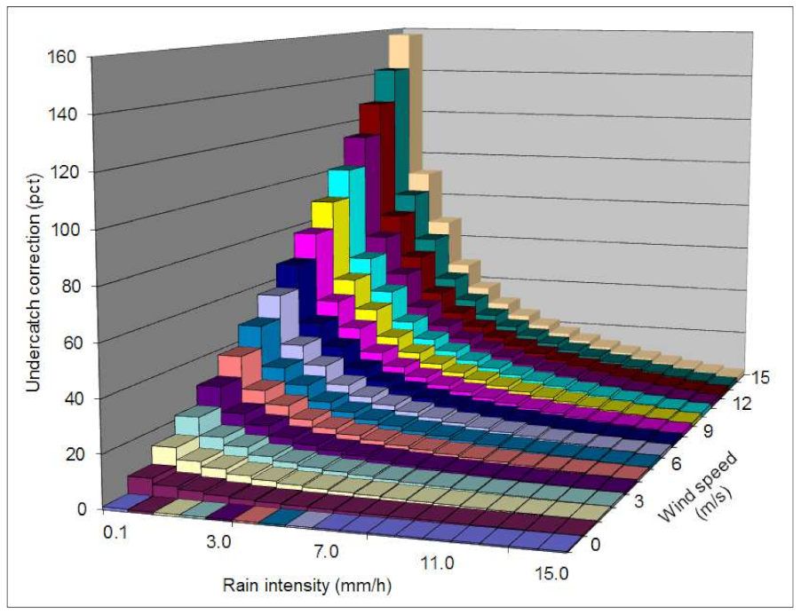
The relation between under-catch as a function of rain rate and wind speed at gauge level for rain is shown in Figure 4. It was for unsheltered conditions. It was noticed that for a low rain rate and high wind speed, the correction was extremely high and decreasing with rain rate and wind speed.
The magnitude of the under-catch was linked to the geometry of a rain gauge, i.e., it matters which type of rain gauge is used. At Hvide Sande, a shielded Geonor was installed over the whole period. The windshield reduced the under-catch, and, therefore, we used a model for correction of Geonor data. Hereby, we corrected the measured values to the true amount of precipitation considering the under-catch due to wind.
We made a sensitivity study for Hvide Sande, to find out 2 things: First, how much less rain (under-catch) would have been measured if uncorrected data from a Geonor, Rimco, or Pluvio2 rain gauge had been used instead of the true amount. Second, how much would the lifetime prediction be changed using uncorrected rain data from the 3 types of rain gauges.
To enable this sensitivity study, we calculated the correction as if it would be a Rimco or Pluvio2 type, both unshielded. This gave us 3 corrected precipitation time series: (1) Geonor corrected, (2) Pluvio2 corrected, and (3) Rimco corrected. We expected the under-catch to be smallest for Geonor, then Pluvio2, and most severe for Rimco. Using the time series for the calculation of the time to damage at turbine blades, we assumed to find the longest time to damage for the observed amount and shorter times for corrected values of Geonor, Pluvio2, and Rimco. The wind speed correction on rain was considered only for Hvide Sande, as this was a sensitivity test study.

3. Results

3.1. Results on Site-Specific Variability in Lifetime and Profit from ESM Operation

The results from the analysis on the spatial variability of the rain environmental load were presented for three domains: The North Sea, the Baltic Sea, and inland stations. The average yearly variation of percentage of time of exceedance of rain rate (in mm h−1) for all wind speeds and for wind speeds ≥7 m s−1 are shown in Figure 5. As an example for Aalborg, we see that the rain rate of 10 mm h−1 occurred 0.05% of the time when it rains (left panel), while 10 mm h−1 occurred around 0.008% of the time when it rains and wind speeds were equal to or greater than 7 m s−1. We expected the majority of LEE to be caused by rain events when the turbine was near or at rated speed, i.e., for wind speed corresponding to the rated wind speed of the IEA Wind 15 MW turbine. The exceedance curves do not show the absolute sum of rain but the percentage of time with rain for specific rain rates.
For the stations around the North Sea, high rain rates concurrent with high wind speeds were most frequent at Helgoland and List, and least at Utsira and Weybourne. The other stations’ data fell in between. The mean annual precipitation at Utsira was higher than at all other stations (Figure 2), and the higher exceedance curve at Utsira confirms this (Figure 5). It is interesting to notice that the exceedance of Utsira was particularly high for rain rates from 0.1–8.0 mm h−1 but not for rain rate 10 mm h−1 and above. Thus, the rain rate and wind speed statistics differed between Utsira and the Danish and German North Sea stations.
Weybourne stands out with very high exceedance rain rates from 0.1–8.0 mm h−1 but not for rain rate 10 mm h−1 and above. It is surprising that the rain rates frequently occurred in a relatively dry region, but it may be due to the measurement technique or duration of measurements (see details in section discussion).
For the stations around the Baltic Sea, the statistics were similar for all four stations. The percentage of time with exceedance rates for high rain rates was marginally lower than for the North Sea.
The variation in rain rate was very large for the inland stations. Billund and Karup have very few occurrences of high rain rates during high wind speed, while Grosser Arber and Bremen frequently have high rain rates during high wind speeds, around the same values as for the North Sea stations. Grosser Arber was located at a high elevation in a mountaineous area.
Investigation of the time to damage using the damage model [15] and the assumptions for ESM operation following [18] was calculated. Three cases were modeled for all 18 stations (see Section 2.5).
The idealized case has an infinite lifetime, and there is no loss in AEP due to erosion. The ideal AEP was entirely dependent on the wind climate. Figure 6 shows the ideal AEP per station with the grouping of the eight North Sea stations, four Baltic Sea stations, and six inland stations. As expected, the North Sea stations have higher production (average 83 GWh) than the Baltic Sea stations (average 71 GWh) and the inland stations (average 44 GWh), even though Grosser Arber in the mountains have high AEP.
The default case has lower AEP than the idealized case due to erosion of the blades. The percentage loss in AEP comparing the idealized case and the default case was on average 0.46% (as already noted in the introduction). There was only modest variation between the stations. The averages were 0.40% for the North Sea stations, 0.50% for the Baltic Sea stations, and 0.63% for the inland stations (Table 2). The AEP loss quantifies the effect of the assumptions between the ideal power curve and the eroded power curve, described in Section 2.5.
The lifetime for the default case was calculated for each station, and the result is shown in Figure 7. The average lifetime was 5.2 years. There was a very large variation between the stations. The shortest lifetime was 0.9 years at Grosser Arber (it may be noted the wind is relatively high), and the longest was 27.9 years at Weybourne. Utsira had the second longest lifetime (13.3 years).
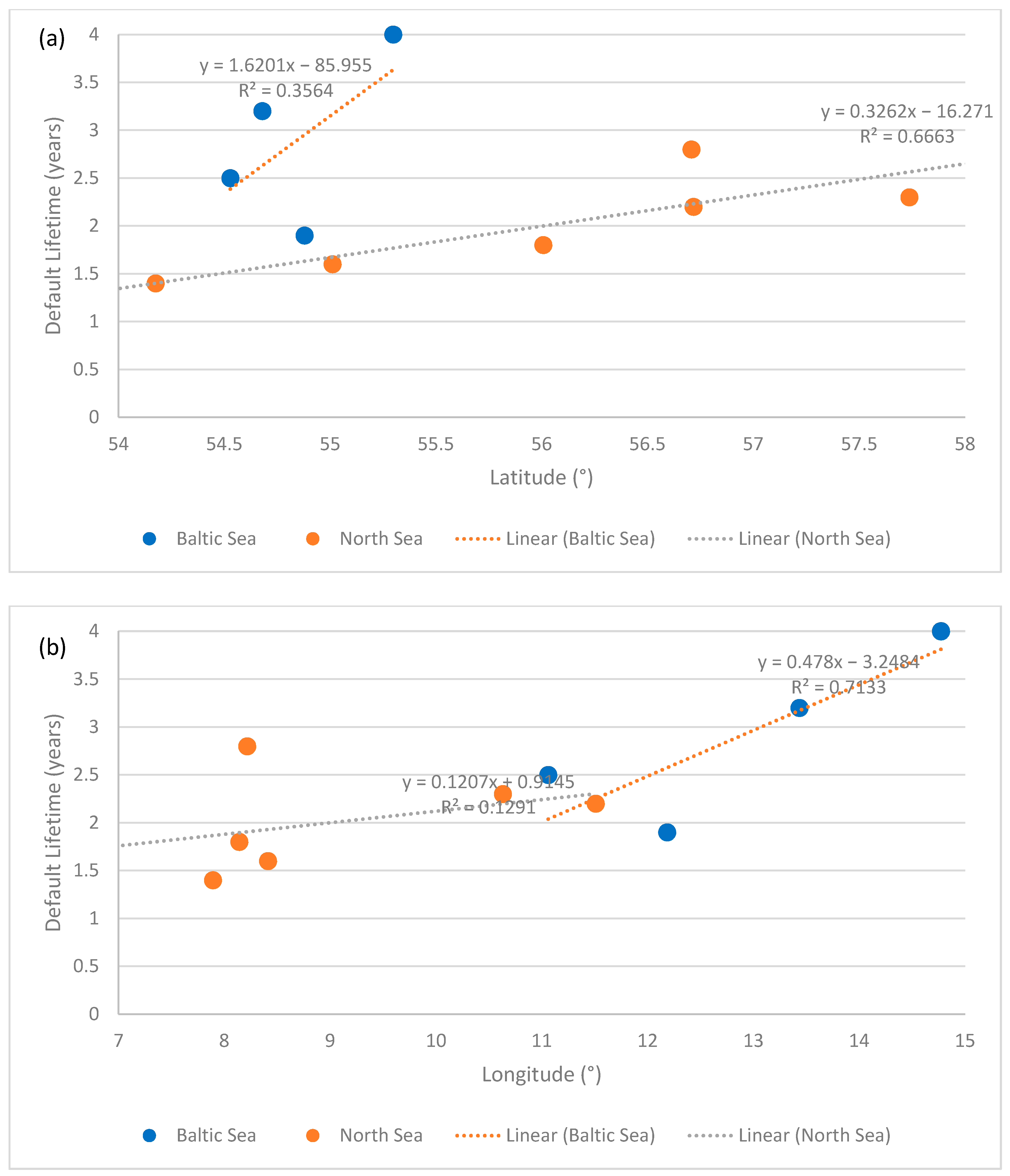
The average lifetime for all North Sea stations was 6.7 years in default operation. Excluding Utsira and Weybourne and only averaging for the North Sea stations in Denmark and Germany showed 2.0 years lifetime on average. Among the Danish and German North Seas stations, the shortest lifetime was at Helgoland (1.4 years), followed by List (1.6 years), Hvide Sande (1.8 years), and the longest at Thyborøn (2.8 years). There appeared to be a South to North gradient with a longer lifetime in the North.
The variability in a lifetime for the Baltic Sea stations in default operation was on average 2.9 years. The minima were Vindebæk (1.9 years) and Fehmarn (2.5 years), located in the western part of the Baltic Sea. The maxima were Arkona (3.2 years) and Hammerodde (4.0 years), located further east. There appeared to be a West to East gradient with a longer lifetime in the East. The western Baltic Sea stations have comparable lifetimes to the North Sea stations Skagen (2.3 years) and Anholt (2.2 years).
The inland stations showed on average 4.6 years lifetime in default operation and with large variability among stations ranging from minimum 0.9 years at Grosser Arber to maximum 10.7 years at Karup. In Figure 5 we see that heavy rain at wind speeds ≥7 m s−1 was more frequent at Grosser Arber than at Karup, which helps us to understand this difference.
The variation in a lifetime along the South-North (latitudes) and West-East (longitudes) gradient for the Danish and German coastal stations was studied. Figure 8 shows increasing lifetime from South to North with linear regression R2 at 0.67 in the North Sea and increasing lifetime from West to East with R2 at 0.71 in the Baltic Sea.
The ESM operation was investigated in different ways. First, the calculation of lifetime for ESM was done using a threshold rain rate at 10 mm h−1 and tip speed at 73 m s−1 for all stations. The average lifetime was found to be 19.8 years. In case more radical thresholds are selected, longer lifetimes will be found. In case more conservative thresholds are selected, shorter lifetimes will be found. For very mild thresholds, lifetime will approach the default lifetime.
Based on the mentioned thresholds, the profit for idealized case vs. default case was reported for each station. The percentage profit was normalized with the default profit. The results are listed in Table 2.
The idealized case was valid for perfect infinitely durable blades. The default case was for gradually eroding blades and assumed repair to be done when the damage had reached a certain threshold. There was some variation between stations with very low values for Weybourne and Utsira. This was consistent with long lifetimes at those two sites, such that AEP loss due to rougher blades was limited. At the other end of the scale, Grosser Arber and Bremen showed large differences in profit. Results using threshold rain rate at 10 mm h−1 and tip speed at 73 m s−1 for all stations was on average giving a profit at 0.77% default vs. ESM operation.
The purpose of the ESM operation was to optimize profit. Even more profit can be obtained from ESM operation than described above. This can be done using site-specific optimization of the ESM threshold values based on the site-specific rain and wind statistics at each site. Thus, instead of the 10 mm h−1 and tip speed at 73 m s−1 thresholds, new values for each site were calculated. Using the optimized threshold values in the damage model, the average profit was 0.98% (compared to 0.77%). The profit values in % for each station are shown in Figure 9 and listed in Table 3. The damage model optimized thresholds rain rate values varied from 3.0 to 6.7 mm h−1 and tip speed values from 63.0 to 70 m s−1 between the stations with an average rain rate at 4.06 mm h−1 and tip speed at 67.5 m s−1. Figure 9 also shows the idealized profit vs. default.
Erosion caused 1.41% profit loss for the 18 stations. In case site-specific optimized ESM operation would be performed, the profit for all 18 stations was 0.98%. Thus, around 70% of the profit loss due to LEE might be gained using site-specific optimized ESM operation. The remaining 30% loss in profit only ideal blades can provide, not ESM. As an example, for Anholt, an IEA 15 MW turbine with ideal blades with infinite lifetime would give 1.33% more profit than default operation. Optimized ESM operation would give 1.06% more profit than default operation. Thus, 0.27% loss in profit cannot be gained from ESM operation but only from ideal blades.

3.2. Results on Sensitivity to Length of Time Series for Predicted Lifetime

The sensitivity to the length of time series was analyzed for station Hvide Sande.
The results for sampling 2 out of 18 years and for sampling 16 out of 18 years for the percentage of time the rain rate was exceeded is shown in Figure 10. The sensitivity to the length of time series showed the largest variation for the highest rain rate as expected. It was clearly seen for the 2-year sample size. Light rain occurred more often than heavy rain. Thus, the spread in data (the black dots) was much larger for heavy rain than for light rain. When the 16-year sample was used, the spread in rain rate data was low.
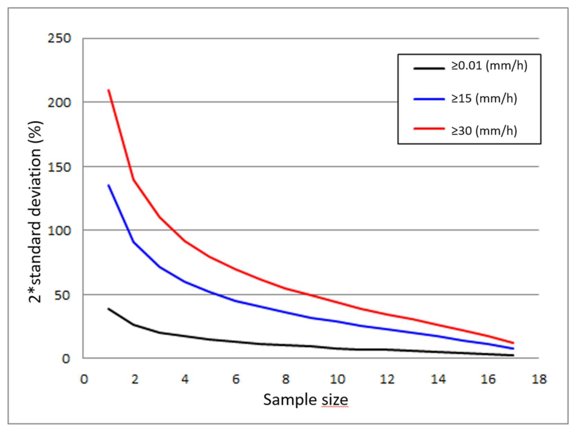
Another way of presenting the variation in rain rate distribution with sample size was to keep the rain rate constant and see the variation with sample size. Here, the three rain rates (≥0.01 mm h−1, ≥5 mm h−1, and ≥30 mm h−1) were selected, and +2 standard deviations (wet conditions) for 17 different sample sizes from 1 to 17 years for all data are shown in Figure 11. It was seen again that at low rain rates, the variation was small, but for high rain rates and short sampling period, the variation was very high. As an example, for the rain rate ≥15 mm h−1, the 1-year sample size showed more than 100% variation for 2 standard deviations and for 5-year sample size around 50% variation.
The overall purpose of the sensitivity analysis on sample size and rain rate was to investigate the influence on the calculation of lifetime. This was done using the corresponding representative time series from 1 to 17 years. The entire 18 years was used as the reference. The representative time series were ±2 standard deviations (wet and dry conditions). The result is presented in Figure 12.
The default lifetime assuming default operation was 1.8 years (grey dot) in Figure 12. For very dry conditions (red dots), the lifetime was much longer, up to 12.2 years for the shortest sample size (1 year). In contrast, for very wet conditions (blue dots), the lifetime was shorter, down to 1.0 year for the shortest sample size. To visualize the tendency, logarithmic trend lines are included in Figure 12. The lifetime calculated for very dry conditions deviated nearly an order of magnitude from the reference, while during very wet conditions, the deviation was around 50%. In other words, for the very dry conditions, there was more than 10 years difference compared to the reference lifetime, while for very wet conditions, there was only 0.6 years difference compared to the reference lifetime. Interestingly, only minor deviation from the reference lifetime was found for 10-year sample sizes and above.
In summary, the results showed that if measurements were available only from few very dry years, the lifetime would be severely over-estimated. Should a sampling period with few very wet years be available, the lifetime was likely to be estimated with values close to the reference lifetime.
The ideal AEP as a function of sample size for ±2 standard deviation rain rate was also presented in Figure 12 (note the secondary y-axis). The reference ideal AEP (grey triangle) was 80 GWh. The results show that higher AEP was found for very wet conditions (blue triangles) and lower AEP for dry conditions (red triangles). The ideal AEP was independent of rain as the blades were assumed to have an infinite life and a clean power curve. Thus the result was telling that the weather conditions were characterized by low winds during very dry conditions and high winds during very wet conditions.
With 10 years and longer time series, the results appeared robust compared to the reference values for a lifetime and for AEP.
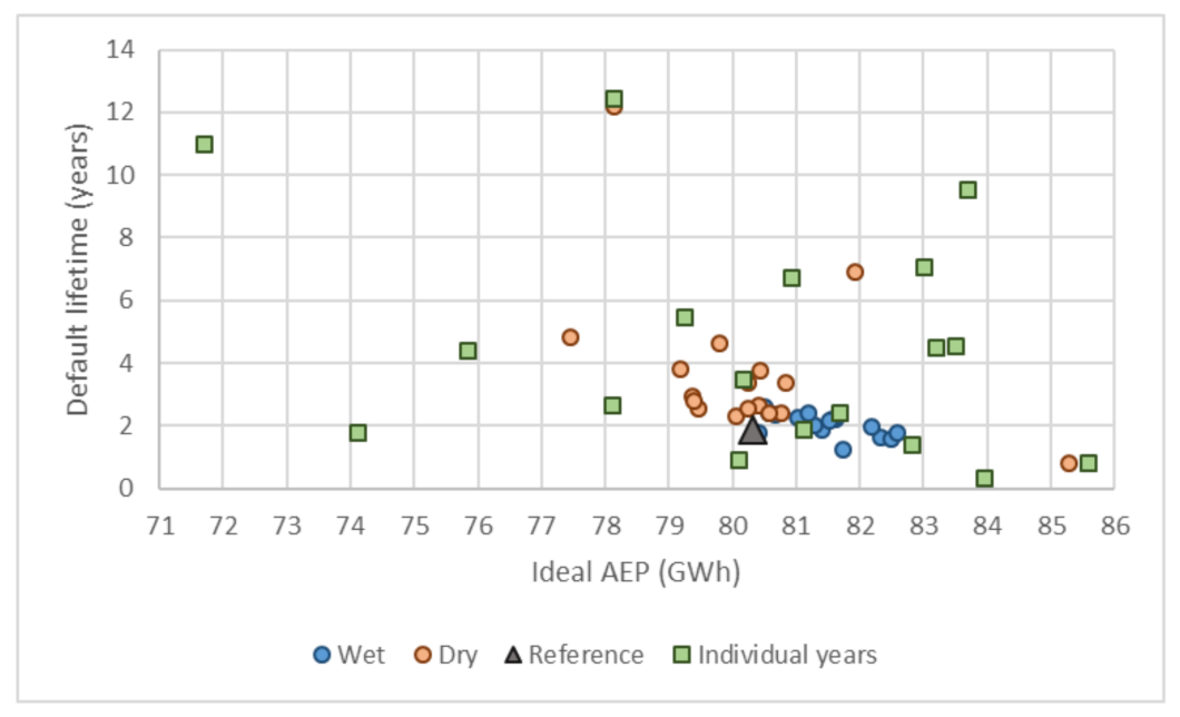
The scatterplot in Figure 13 shows the ideal AEP and default lifetime for the same data as in Figure 12. The very wet samples (blue dots) clustered near the reference value (grey triangle) while the very dry samples (red dots) mainly over-predicted the lifetime compared to the reference lifetime.
The green squares in Figure 13 show results based on individual years at Hvide Sande from 2002 to 2019. This was an alternative way of investigating how the lifetime prediction may vary depending upon sampling size (1 year). The reference lifetime based on 18 years of data was 1.8 years, while the average lifetime from 18 individual years was 4.5 years. There was a clear tendency to overestimate lifetime using a short sampling size. The scatterplot in Figure 13 shows that not only default lifetime but also ideal AEP vary greatly from year to year.

3.3. Results on Wind Speed Correction of Rain Rate Observations and Predicted Lifetime

The rain-rate time series from station Hvide Sande during 18 years was corrected for wind speed, which gives the true rain rate. The sensitivity study on uncorrected rain data assuming three different rain gauges types were reported. Table 4 shows the rain amount after correction. It was found that Rimco would have the largest under-catch both for average per year (11.2%) and in particular in the months with highest wind speeds, namely December, January, and February (14.5%). Average rain rates were lowest in February and highest in August.
The effect of under-catch to the assessment of the lifetime considering three rain gauge types were calculated. The results were for Geonor 1.84 years, Pluvio2 1.78 years and Rimco 1.75 years, respectively. In other words, the under-catch correction for Rimco would result in 5% under-prediction of lifetime. Thus, under-catch of rain during high wind speed would be important to correct to accurately assess LEE. Often though, information is not available to conduct the correction. It should be kept in mind that under-catch of rain will overestimate lifetime.

4. Discussion

The rain erosion environmental load based on many years of rain rate and wind speed observations for 18 sites in Denmark, Germany, Norway, and the UK is reported. The statistics on the percentage of time rain-rate exceedance thresholds provide a qualitative description. Low rain-erosion potential is found at stations with few occurrences of high rain rates concurrent with high wind speeds. High rain-erosion load potential is generally found at stations showing frequent high rain rates concurrent with high wind speed. The rain-rate exceedance diagrams for wind speed above specific thresholds can be used as an indication of the rain-erosion load differences between stations. It may be noted though that the rain rate percentage exceedance curves are not absolute but relative. The annual average rainfall amount varies between stations (indicated in Figure 2). In Denmark, Billund has a higher annual average mean rainfall than the other two inland stations (Aalborg and Karup) [38], and, therefore, a shorter default lifetime.
The more advanced method to assess the rain erosion environmental load is to use a damage model and predict the expected lifetime of the leading edge of blades. The damage progression is a function of rain rate and tip speed and is a non-linear process. The examples using the IEA Wind 15 MW reference wind turbine for calculation of LEE show the Danish and German stations near the North Sea to have an average lifetime of 2.0 years and the Baltic Sea 2.9 years.
Interestingly, the data indicate a South to North gradient in lifetime along the German and Danish North Sea coastline at stations Helgoland, List, Hvide Sande, and Thyborøn with increasing lifetime towards the North. Weather systems from Southwest, West, and Northwest bring most of the rain [39]. The mountains in Norway reduce the rain amount at the Danish stations, most pronounced in northern Denmark during northwesterly flows. This may be a reason for the South to North gradient in lifetime.
The Baltic Sea stations indicate a West to East gradient in lifetime from Vindebæk and Fehmarn in the West and increasing lifetime towards the East at Arkona and Hammerodde. The annual precipitation at Hammerodde is lower than Vindebæk [38] and a higher percentage rain rate exceedance is seen for Vindebæk and Femarn than Hammerodde, so the main reason for the gradient in lifetime is probably due to differences in rain climates in the Baltic Sea.
At Weybourne, a very long lifetime is calculated (27.9 years). The atlas on rainfall over the North Sea based on satellite data from 1979–1996 shows a low mean annual rainfall in the area near Weybourne [40]. This is also supported by satellite data from 1988 to 2008 [22], see Figure 2, and from station data [41]. The deviation from Weybourne compared to the other North Sea station in relation to the rain-rate exceedance curves and lifetime might also be caused due to the much shorter time series compared to the other stations (2.5 vs. > 10 years), including the exceptional dry year 2018. Furthermore, it may be that disdrometers have a positive bias in the rain rate measurements compared to classical rain gauges [42].
At Utsira, a long lifetime is calculated (13.3 years). The mean annual rainfall at Utsira is very high [22,40], which could indicate shorter lifetime than at the Danish and German coastal stations. However, the rain rate exceedance threshold diagrams (Figure 5) clearly show that rainfall at rain rates between 0.1–8.0 mm h−1 is abundant while a rain rate above 10 mm h−1 is below the exceedance curves for the Danish and German stations in the North Sea. This is most clear for all wind speeds but also for wind speeds ≥7 m s−1.
The time series at Weybourne and Utsira are 2.6 and 3.3 years, respectively. These are much shorter than at the other stations investigated (from 13 to 28 years). Obviously it is easier to accurately predict a recurring episode or condition that takes place several times within a given observation time series, than extrapolating far beyond the length of the given time series. The sensitivity analysis based on 18 years of data from station Hvide Sande shows that both default lifetime and ideal AEP are represented well by time series of 10 years and longer but deviates much from the reference values for shorter time series. In case the time series is only one-year long, over-prediction of lifetime is very likely to happen (it occurred 12 out of 18 times in the sensitivity test). In case the short time series represent very dry conditions, the lifetime will be severely over-predicted. The inter-annual variability on lifetime indicates that the damage processes may differ much between years.
The sensitivity analysis on correction of measured rain gauge data for wind speed indicates that under-catch—if not corrected for—will result in over-prediction of lifetime.
The lifetimes calculated for Weybourne and Utsira could well be over-predicted due to a short time series and possible under-catch if not properly corrected for. In case the lifetime at Utsira represents the true average lifetime, the South to North gradient in average lifetime increasing from Helgoland in Germany to Thyborøn in Denmark can be extended up to Utsira with much longer lifetime at the Norwegian coast. It should be noted that rainfall under-catch potentially could change the results on expected lifetime between stations. The sensitivity results on wind speed correction for rainfall, for example at station Hvide Sande, show a difference of around 5% in lifetime between different types of rain gauges. The correction for rainfall under-catch is based on independent, international research [31,32,33] and on-going research at DMI on under-catch by Pluvio suggests a higher underestimation than our results show, i.e., lifetime may be over-predicted if not properly accounted for.
The lifetime at inland stations varies much. At Aalborg and Karup in Denmark, much longer lifetimes compared to the Danish coastal stations are found. The result is consistent with analysis from a shorter period, using another wind turbine as an example and extrapolation of winds to hub height including terrain and roughness effects [17]. A study in the Netherlands also found shorter lifetime near the coastline than inland [9]. Grosser Arber has a very short lifetime and high AEP. This station is located at a mountain with higher winds than the other inland stations.
The widespread repair of blades indicate that LEE is a challenge. Mitigation strategies can involve new coatings and ESM operation, or a combination of the two.
Our calculations shows that LEE causes an average loss in AEP of around 0.46%. This loss is due to lower aerodynamic performance due to eroded blades. Our value is small compared to cited values on AEP loss from aerodynamic performance, e.g., 5% [43], 2% to 3.7% [44], 1.8% to 4.9% [45], and 1.5% [7]. We assume repair to take place before very serious damage occurs. Our results on potential profit using ESM operation are conservative. In case we use the cited values above, the profit loss between ideal blades and default operation would be larger, and the potential benefit of ESM operation larger.
The eroded power curve we use from [18] could be elaborated to include an initial incubation phase, and other subsequent phases in the LEE process [1,4,7,43]. Furthermore, damage caused by solid precipitation such as graupel, ice pellets, and hailstones could be included as their kinetic impact can be high [4,5]. Hail is short-lived and not frequent over the European seas [46]. Most likely it would be best to stop turbines during hail events to extend the blade lifetime.
To enable ESM operation at a turbine, there is need for real-time observation of rain rate. This could be from a Micro Rain Radar [47] that would allow control much faster than at 10-minute intervals for initiation and completion of ESM for each rain event. Thus, the calculations reported above might be optimized further using shorter time scales than 10 minutes. Rain events can be of shorter duration than 10 minutes and with variability within 10 minutes [48]. Therefore, less time in ESM operation might be relevant.
Furthermore, adding the complexity of farm control (e.g., wake steering, load reduction) to the equation on optimization for LEE could be a relevant avenue for research and optimization. The cost modeling using fluctuating energy market spot price [18] and forecasting of rain events jointly with power production forecasting could be combined for future wind farm operation.
The lack of rain rate data across the seas is a fundamental problem for predicting offshore rain erosion environmental load accurately. Ground-based radar network for offshore rain rate mapping could support this [39]. A couple of strategically located weather radars at platforms in the North Sea could provide 5-minute nowcasting of precipitation type and rain rate. These radars at sea should be operated in combination with the weather radars in neighboring countries to cover the relevant sea optimally. Radars in midland US have been used to quantify rain and hail events for LEE [49], but similar results for offshore are not (yet) available.
ESM operation should be optimized for each specific site. However, as relevant data are lacking, it might become relevant to use proxy values. This might be from numerical weather model results but typically at lower temporal resolution. Using input data with lower temporal resolution adjustments to the damage model would be necessary, as lifetime otherwise would be over-predicted. Observations from satellites could also be considered, e.g., combining the various satellite sources providing rain parameters [22,40,50] with concurrent satellite-based winds.

5. Conclusions

Conclusions based on the analysis of rain rate and wind speed time series for rain erosion environmental load, default blade lifetime, and potential profit are:
  • Time series of more than 10 years duration appear to give robust results on blade lifetime, while shorter time series are likely to over-predict blade lifetime.
  • Correction for wind speed on rain amount for specific rain gauge types is relevant as the uncorrected (under-catch time series) will over-predict blade lifetime.
Assuming an IEA Wind 15 MW reference wind turbine is installed at each of the stations shows the following lifetimes, based on the damage model:
  • The lifetime increases from the South to the North along the German and Danish North Sea coastline: Helgoland (1.4 years), List (1.6 years), Hvide Sande (1.8 years), and Thyborøn (2.8 years). The time series are from 18 to 23 years long.
  • The lifetime increases from the West to the East in the Baltic Sea: Fehmarn (2.5 years) and Vindebæk (1.9 years) in the western part while Arkona (3.2 years) and Hammerodde (4.0 years) are located further East. The time series are from 13 to 28 years long.
  • Weybourne’s lifetime (27.9 years) calculated from a time series of 2.6 years duration may be over-predicted. Weybourne is located in a region with low annual rainfall, thus a longer lifetime than in the eastern part of the North Sea appears likely.
  • Utsira’s lifetime (13.3 years) calculated from a time series of 3.3 years may also be over-predicted. In contrast to Weybourne, Utsira is located in a region with very high annual rainfall. Thus further analysis is needed to conclude on the lifetime, if lifetime is truly much longer than in the Danish North Sea.
LEE causes an average loss in AEP of around 0.46%. This loss is due to lower aerodynamic performance due to eroded blades.
The loss in profit due to LEE is on average 1.51% for the Danish and German North Sea stations, and 1.35% for the Baltic Sea stations comparing to ideal blades with infinite lifetime. It would be possible to gain around 70% of this loss using erosion-safe mode operation, i.e., adjust the tip speed during heavy rain events to reduce blade erosion, aerodynamic loss, repair costs, and downtime during repair.

Author Contributions

C.B.H. had the lead on writing the paper and calculating lifetime and profit. F.V. contributed to rain and wind data analysis. W.R.S. programmed the damage model and optimization. A.-M.T. contributed to rain and wind data analysis. All contributed to writing the paper. All authors have read and agreed to the published version of the manuscript.

Funding

This work was supported by the Innovation Fund Denmark Grant 6154-00018B for the project EROSION.

Data Availability Statement

The meteorological data used in this study are openly available in the Natural Environment Research Council’s Data Repository for Atmospheric Science and Earth Observation (CEDA), the Danish Meteorological Institute’s (DMI) Frie Data repository, the German Weather Service (DWD) Climate Data Center, and The Norwegian Meteorological Institute (NMI) based on data from MET Norway.

Acknowledgments

Permission to use Figure 2 produced by DWD is kindly granted by M. Quante. Meteorological data from the Open Data Server of Deutscher Wetterdienst, the Norwegian Meteorological Institute, the Meteorological data from the Natural Environment Research Council and the Danish Meteorological Institute are acknowledged. We acknowledge the anonymous reviewers that helped us to improve the paper.

Conflicts of Interest

The authors declare that they have no conflict of interest.

Appendix A

Table A1. Empirical constants for solid and liquid precipitation for three rain gauge types: Geonor, Pluvio2, and Rimco [28,30,31]. Empirical constants for the manual Danish Hellmann rain gauge are assumed to be representative for Pluvio2 as proposed in [35]. Ongoing research at DMI reveals that using these constants the undercatch correction of Pluvio2 may be slightly underestimated.
Precipitation TypeSymbolRimco, Pluvio2Geonor, Shielded
Snowβ00.04587−0.12159
β10.236770.18546
β20.0179790.006918
β3−0.015407−0.005254
Rainγ00.0076970.007697
γ10.0343310.034331
γ2−0.00101−0.00101
γ3−0.012177−0.012177
c0.0−0.05

References

  1. Slot, H.M.; Gelinck, E.R.M.; Rentrop, C.; van der Heide, E. Leading edge erosion of coated wind turbine blades: Review of coating life models. Renew. Energy 2015, 80, 837–848. [Google Scholar] [CrossRef]
  2. Eisenberg, D.; Laustsen, S.; Stege, J. Wind turbine blade coating leading edge rain erosion model: Development and validation. Wind Energy 2018, 21, 1–10. [Google Scholar] [CrossRef]
  3. Punge, H.J.; Kunz, M. Hail observations and hailstorm characteristics in Europe: A review. Atmos. Res. 2016, 176–177, 159–184. [Google Scholar] [CrossRef]
  4. Keegan, M.H.; Nash, D.; Stack, M. On erosion issues associated with the leading edge of wind turbine blades. J. Phys. D Appl. Phys. 2013, 46, 383001. [Google Scholar] [CrossRef] [Green Version]
  5. Letson, F.; Barthelmie, R.J.; Pryor, S.C. Radar-derived precipitation climatology for wind turbine blade leading edge erosion. Wind Energy Sci. 2020, 5, 331–347. [Google Scholar] [CrossRef] [Green Version]
  6. Macdonald, H.; Infield, D.; Nash, D.H.; Stack, M.M. Mapping hail meteorological observations for prediction of erosion in wind turbines. Wind Energy 2016, 19, 777–784. [Google Scholar] [CrossRef] [Green Version]
  7. Papi, F.; Balduzzi, F.; Ferrara, G.; Bianchini, A. Uncertainty quantification on the effects of rain-induced erosion on annual energy production and performance of a Multi-MW wind turbine. Renew. Energy 2021, 165. [Google Scholar] [CrossRef]
  8. Prieto, R.; Karlsson, T. A model to estimate the effect of variables causing erosion in wind turbine blades. Wind Energy 2021, 22, 1–14. [Google Scholar] [CrossRef]
  9. Bartolomé, L.; Teuwen, J. Methodology for the energetic characterisation of rain erosion on wind turbine blades using meteorological data: A case study for The Netherlands. Wind Energy 2021, 1–13. [Google Scholar] [CrossRef]
  10. Dashtkar, A.; Hadavinia, H.; Sahinkaya, M.N.; Williams, N.A.; Vahid, S.; Ismail, F.; Turner, M.A.; Vahid, S.; Ismail, F.; Turner, M. Rain erosion-resistant coatings for wind turbine blades: A review. Polym. Polym. Compos. 2019, 27, 443–475. [Google Scholar]
  11. Herring, R.; Dyer, K.; Martin, F.; Ward, C. The increasing importance of leading edge erosion and a review of existing protection solutions. Renew. Sustain. Energy Rev. 2019, 115, 109382. [Google Scholar] [CrossRef]
  12. Mishnaevsky, L., Jr. Repair of wind turbine blades: Review of methods and related computational mechanics problems. Renew. Energy 2019, 140, 828–839. [Google Scholar] [CrossRef]
  13. IEA International Energy Agency Offshore. Wind Outlook 2019, World Energy Outlook Special Report, Technology report—November. Available online: https://www.iea.org/reports/offshore-wind-outlook-2019 (accessed on 31 March 2021).
  14. Wind Europe. Our Energy, Our Future, How Offshore Wind Will Help Europe Go Carbon-Neutral. 2019. Available online: https://windeurope.org/about-wind/reports/our-energy-our-future/ (accessed on 31 March 2021).
  15. Bech, J.I.; Hasager, C.B.; Bak, C. Extending the life of wind turbine blade leading edges by reducing the tip speed during extreme precipitation events. Wind Energ. Sci. 2018, 3, 729–748. [Google Scholar] [CrossRef] [Green Version]
  16. Hasager, C.B.; Vejen, F.; Bech, J.I.; Skrzypiński, W.R.; Tilg, A.-M.; Nielsen, M. Assessment of the rain and wind climate with focus on wind turbine blade leading edge erosion rate and expected lifetime in Danish Seas. Renew. Energy 2020, 149, 91–102. [Google Scholar] [CrossRef]
  17. Skrzypiński, W.R.; Bech, J.I.; Hasager, C.B.; Tilg, A.-M.; Bak, C. Optimization of the erosion-safe operation of the IEA Wind 15 MW Reference Wind Turbine. J. Phys: Conf. Ser. 2020, 1618, 052034. [Google Scholar] [CrossRef]
  18. Bak, C.; Forsting, A.M.; Sørensen, N.N. The influence of leading edge roughness, rotor control and wind climate on the loss in energy production. J. Phys. Conf. Ser. 2020, 1618. [Google Scholar] [CrossRef]
  19. Gaertner, E.; Rinker, J.; Sethuraman, L.; Zahle, F.; Anderson, B.; Barter, G.; Abbas, N.; Meng, F.; Bortolotti, P.; Skrzypiński, W.R.; et al. Definition of the IEA 15-Megawatt Offshore Reference Wind Turbine (NREL/TP-5000-75698); National Renewable Energy Laboratory: Golden, CO, USA. Available online: https://www.nrel.gov/docs/fy20osti/75698.pdf (accessed on 31 March 2021).
  20. Nešpor, V.; Sevruk, B. Estimation of Wind-Induced Error of Rainfall Gauge Measurement Using a Numerical Simulation. J. Atmos. Ocean. Technol. 1999, 16, 450–464. [Google Scholar] [CrossRef]
  21. Natural Environment Research Council; Met Office; Pickering, B.S.; Neely, R., III; Harrison, D. The Disdrometer Verification Network (DiVeN) Particle Diameter and Fall Velocity Measurements from a Network of Thies Laser Precipitation Monitors Around the UK (2017–2019); Centre for Environmental Data Analysis: Chilton, UK, 2019. [Google Scholar] [CrossRef]
  22. Quante, M.; Colijn, F.; Bakker, J.P.; Härdtle, W.; Heinrich, H.; Lefebvre, C.; Nöhren, I.; Olesen, J.E.; Pohlmann, T.; Sterr, H.; et al. Introduction to the Assessment—Characteristics of the Region. In North Sea Region Climate Change Assessment, Regional Climate Studies; Quante, M., Colijn, F., Eds.; Springer: Cham, Switzerland, 2016. [Google Scholar] [CrossRef] [Green Version]
  23. Tilg, A.-M.; Skrzypiński, W.R.; Hasager, C.B. Effect of drop-size parametrization and rain amount on blade-lifetime calculations considering leadindg-edge erosion. Wind Energy 2021. in review. [Google Scholar]
  24. Bak, C.; Skrzypiński, W.; Fischer, A.; Gaunaa, M.; Brønnum, N.F.; Kruse, E.K. Wind tunnel tests of an airfoil with 18% relative thickness equipped with vortex generators. J. Phys. Conf. Ser. 2018, 1037. [Google Scholar] [CrossRef]
  25. Best, A.C. The size of distribution of raindrops. Quart. J. R. Met. Soc. 1950, 76, 16. [Google Scholar] [CrossRef]
  26. Brualdi, R.A. Introductory Combinatorics, 5th ed.; Pearson Prentice Hall: Upper Saddle River, NJ, USA, 2010; ISBN 978-0-13-602040-0. [Google Scholar]
  27. Sevruk, B.; Hamon, W.R. International Comparison of National Precipitation Gauges with a Reference Pit Gauge; World Meteorological Organization: Geneva, Switzerland, 1984. [Google Scholar]
  28. Goodison, B.E.; Louie, P.Y.T.; Yang, D. WMO Solid Precipitation Measurement Intercomparison: Final Report. Instruments and Observing Methods, Report No. 67 (WMO/TD No. 872); World Meteorological Organization: Geneva, Switzerland, 1998. [Google Scholar]
  29. Allerup, P.; Madsen, H. Accuracy of point precipitation measurements. Nord. Hydrol. 1980, 11, 57–70. [Google Scholar] [CrossRef]
  30. Allerup, P.; Madsen, H.; Vejen, F. A Comprehensive Model for Correcting Point Precipitation. Nord. Hydrol. 1997, 28, 1–20. [Google Scholar] [CrossRef]
  31. Sevruk, B.; Klemm, S. Types of standard precipitation gauges. In Proceedings of the WMO, IAHS, ETH International Workshop on Precipitation Measurement, St. Moritz, Switzerland, 3–7 December 1989; pp. 227–232. [Google Scholar]
  32. Allerup, P.; Dahlström, B.; Elomaa, E.; Jónsson, T.; Madsen, H.; Perälä, J.; Rissanen, P.; Vedin, H.; Vejen, F. Manual for Operational Correction of Nordic Precipitation Data (Nordic Working Group on Precipitation, Report Nr. 24/96), 1st ed.; Førland, E.J., Ed.; DNMI: Copenhagen, Denmark, 1996; pp. 1–66. [Google Scholar]
  33. Rasmussen, R.; Baker, B.; Kochendorfer, J.; Meyers, T.; Landolt, S.; Fischer, A.P.; Black, J.; Thériault, J.M.; Kucera, P.; Gochis, D.; et al. How well are we measuring snow? The NOAA/FAA/NCAR Winter Precipitation Test Bed. BAMS 2012, 811–829. [Google Scholar] [CrossRef] [Green Version]
  34. Niemczynowicz, J. Dynamic calibration of tipping-bucket rain gauges. Nord. Hydrol. 1986, 17, 203–214. [Google Scholar] [CrossRef]
  35. Vejen, F.; Vilic, K.; Jensen, H.; Kern-Hansen, C. Korrigeret Nedbør 1989–2010, 2011–2012 & 2013—Konsulentopgave Udført for Dce—Nationalt Center for Miljø Og Energi, Aarhus Universitet, DMI Technical Report, Tr14-13; Danish Meteorological Institute: Copenhagen, Denmark, 2014; pp. 1–228. [Google Scholar]
  36. Sevruk, B. Wind speed estimation at precipitation gauge orifice level. In Instruments and Observing Methods, Report No. 33, Proceedings of the WMO Technical Conference on Instruments and Methods of Observation (TECO-1988), Leipzig, Germany, 16–20 May 1988; World Meteorological Organization (WMO): Geneva, Switzerland, 1988; p. 4. [Google Scholar]
  37. World Meteorological Organization. WMO Guide to Meteorological Instruments and Methods of Observation, WMO-No. 8, 7th ed.; Secretariat of the World Meteorological Organization: Geneva, Switzerland, 2008. [Google Scholar]
  38. Frich, P.; Rosenørn, S.; Madsen, H.; Jensen, J.J. Observed Precipitation in Denmark, 1961–90; Technical Report 97-8; Danish Meteorological Institute, Ministry of Transport: Copenhagen, Denmark, 1997; Available online: https://www.dmi.dk/fileadmin/user_upload/Rapporter/TR/1997/tr97-8.pdf (accessed on 31 March 2021).
  39. Tilg, A.-M.; Hagen, M.; Vejen, F.; Hasager, C.B. Variation of leading-edge-erosion relevant precipitation parameters with location and weather type. Meteorol. Z. 2021, accepted. [Google Scholar]
  40. Tait, A.B.; Barrett, E.C.; Beaumont, M.J.; Brown, P.A.; Taberner, M.J.; Todd, M.C. Interpretation of an atlas of passive microwave-derived rainfall over the eastern North Atlantic Ocean and North Sea. Int. J. Climatol. 1999, 19, 231–252. [Google Scholar] [CrossRef]
  41. Panagos, P.; Ballabio, C.; Borrelli, P.; Meusburger, K.; Klik, A.; Rousseva, S.; Tadic, M.P.; Michaelides, S.; Hrabalikova, M.; Olsen, P.; et al. Rainfall erosivity in Europe. Sci. Total Environ. 2015, 511, 801–814. [Google Scholar] [CrossRef] [Green Version]
  42. World Meteorological Organization. WMO Field Intercomparison of Rainfall Intensity Gauges. In Instruments and Observing Methods, Report No. 99; WMO/TD-No. 1504; World Meteorological Organization: Geneva, Switzerland, 2009. [Google Scholar]
  43. Sareen, A.; Sapre, C.A.; Selig, M.S. Effects of leading edge erosion on wind turbine blade performance: Effects of leading edge erosion. Wind Energy 2014, 17, 1531–1542. [Google Scholar] [CrossRef]
  44. Han, W.; Kim, J.; Kim, B. Effects of contamination and erosion at the leading edge of blade tip airfoils on the annual energy production of wind turbines. Renew. Energy 2018, 115. [Google Scholar] [CrossRef]
  45. Law, H.; Koutsos, V. Leading edge erosion of wind turbines: Effect of solid airborne particles and rain on operational wind farms. Wind Energy 2020, 23, 10–1955. [Google Scholar] [CrossRef]
  46. Punge, H.; Bedka, K.; Kunz, M.; Werner, A. A new physically based stochastic event catalog for hail in Europe. Nat. Hazards 2014, 1625–1645. [Google Scholar] [CrossRef]
  47. Tilg, A.-M.; Hasager, C.B.; Kirtzel, H.-J.; Hummelshøj, P. Brief communication: Nowcasting of precipitation for leading-edge-erosion-safe mode. Wind Energ. Sci. 2020, 5, 977–981. [Google Scholar] [CrossRef]
  48. Mishnaevsky, L., Jr.; Hasager, C.B.; Bak, C.; Tilg, A.-M.; Bech, J.I.; Rad, S.D.; Fæster, S. Leading edge erosion of wind turbine blades: Understanding, prevention and protection. Renew. Energy 2021, 169, 953–969. [Google Scholar] [CrossRef]
  49. Letson, F.; Shepherd, T.; Barthelmie, R.; Pryor, S.C. WRF Modeling of Deep Convection and Hail for Wind Power Applications. J. Appl. Meteorol. Climatol. 2020, 59, 1717–1733. [Google Scholar] [CrossRef]
  50. Rios Gaona, M.F.; Overeem, A.; Leijnse, H.; Uijlenhoet, R. First-Year Evaluation of GPM Rainfall over the Netherlands: IMERG Day 1 Final Run (V03D). J. Hydrometeorol. 2016, 7, 2799–2814. [Google Scholar] [CrossRef]
Figure 1. Map of stations in Denmark, Germany, Norway, and the UK with the North Sea stations in green, Baltic Sea stations in blue, and inland stations in green. The red rectangle indicates the area covered in Figure 2.
Energies 14 01959 g001
Figure 2. Mean annual precipitation totals derived from satellite data showing the spatial distribution of precipitation (mm) across the North Sea region derived from the combined HOAPS-3 and GPCC data set for the period 1988–2008 (figure prepared by the German Meteorological Service, DWD). From [22]. The location of the stations is given.
Energies 14 01959 g002
Figure 3. The clean and eroded power curve for the IEA Wind 15 MW reference turbine. From [18]. Reproduced with permission from Skrzypiński, W.R.; Bech, J.I.; Hasager, C.B.; Tilg, A.-M.; Bak, C. Optimization of the erosion-safe operation of the IEA Wind 15 MW Reference Wind Turbine. J. Phys: Conf. Ser. 1618, 052034, 2020.
Energies 14 01959 g003
Figure 4. Relationship between wind speed, rain rate, and correction in percentage for rain gauge type Pluvio.
Energies 14 01959 g004
Figure 5. The graphs show the average yearly variation of percentage of time of exceedance of rain rates (in mm h−1) for all wind speeds (left panels) and for wind speeds ≥7 m s−1 (right panels) for the North Sea (top), Baltic Sea (middle), and inland stations (bottom).
Energies 14 01959 g005
Figure 6. The ideal Annual Energy Production (AEP) for each station in the North Sea, Baltic Sea, and inland.
Energies 14 01959 g006
Figure 7. The lifetime in default operation for each station in the North Sea, Baltic Sea, and inland.
Energies 14 01959 g007
Figure 8. The default lifetime at Danish and German coastal stations along the North Sea and Baltic Sea as function of (a) latitude and (b) longitude and linear regression results.
Energies 14 01959 g008
Figure 9. The profit (in %) from ideal blades and profit from site-specific optimized erosion-safe mode (ESM) compared to the default case for each station.
Energies 14 01959 g009
Figure 10. The average yearly variation of percentage of time of exceedance of rain rates (in mm h−1) for wind speeds ≥7 m s−1 for entire 18 years (red curve) and with black dots all possible samples of 2 years (left frame) and 16 years (right frame) for Hvide Sande 2002–2019.
Energies 14 01959 g010
Figure 11. The length of time series (sample size) and +2 standard deviations for three rain rates for wind speeds ≥7 m s−1 based on 18 years of rain rate observations at Hvide Sande 2002–2019.
Energies 14 01959 g011
Figure 12. Default lifetime (primary y-axis) and ideal AEP (secondary y-axis) as a function of sample size for Wet (+2 standard deviations) and Dry (−2 standard deviations) on rain rate for 17 different samples sizes and for the Reference (Ref.) of 18 years for Hvide Sande and logarithmic trend lines.
Energies 14 01959 g012
Figure 13. Default lifetime vs. ideal AEP for ±2 standard deviations on rain rate for 17 samples sizes and for the reference of 18 years for Hvide Sande and for each of the 18 individual years from 2002–2019.
Energies 14 01959 g013
Table 1. List of stations, country, data provider, WMO station number, rain gauge type, and period of time series. Tipping bucket according to Joss-Tognini is shortened to Tipping bucket.
LocationCountryData ProviderWMO StationRain Sensor TypeDates (Start, End)Number of Years
AalborgDKDMI603000Theiss, Pluvio28/02/2003, 31/12/201916.9
AnholtDKDMI607900Geonor01/01/2002, 31/12/201917.9
Arkona DEDWD1009100NG 200, Pluvio, rain[e]H301/11/1991, 31/12/201928.2
BillundDKDMI610400Rimco, Pluvio22/08/2003, 31/12/201916.4
BremenDEDWD1022400Tipping bucket, Pluvio29/02/1991, 31/12/201928.2
FehmarnDEDWD1005500Tipping bucket, Pluvio, rain[e]H301/06/1996, 31/12/201923.6
Grosser ArberDEDWD1079100Pluvio, rain[e]H326/02/1998, 31/12/201921.9
HammeroddeDKDMI619300Geonor, Pluvio30/08/2001, 31/12/201918.3
HelgolandDEDWD1001500Tipping bucket, Pluvio20/12/1996, 31/12/201923.0
Hvide SandeDKDMI605800Geonor01/01/2002, 31/12/201918.0
KarupDKDMI606000Rimco, Pluvio13/02/2003, 31/12/201916.9
ListDEDWD1002000Tipping bucket, Pluvio, rain[e]H302/12/1995, 31/12/201924.1
SeehausenDEDWD1026100NG 200, Pluvio, rain[e]H301/11/1991, 31/12/201928.2
SkagenDKDMI604100Geonor01/01/2002, 31/12/201918.0
ThyborønDKDMI605200Geonor, Pluvio01/01/2002, 31/12/201918.0
UtsiraNONMI140300Geonor15/13/1916, 28/06/20193.3
VindebækDKDMI614700Geonor29/05/2006, 31/12/201913.6
WeybourneUKCEDA-Thies LPM22/02/1917, 30/09/20192.6
Table 2. Calculated lifetime for each station for three cases: Ideal, default, and erosion-safe mode (ESM) operation. ESM is calculated with the same threshold values for all stations. Annual Energy Production (AEP) (in GWh) for ideal blades and AEP loss (in %) between ideal blades and default operation are listed.
AreaStationLifetimeAEP
Ideal
(GWh)
AEP Loss
(%)
Ideal
(years)
Default
(years)
ESM
(years)
North Sea Anholt2.213.185.40.35
Helgoland1.49.790.70.26
Hvide Sande1.811.880.30.46
List1.610.287.90.36
Skagen2.313.083.10.43
Thyborøn2.813.677.20.53
Utsira13.362.585.90.04
Weybourne27.945.172.00.07
Average North Sea6.722.482.80.31
Average North Sea DE and DK only2.011.984.10.40
Baltic SeaArkona3.218.372.40.51
Fehmarn2.512.571.60.58
Hammerodde4.020.870.20.32
Vindebæk1.923.868.50.61
Average Baltic Sea2.918.970.70.50
Inland StationsBillund2.814.838.90.52
Bremen1.59.039.20.74
Grosser Arber0.95.368.40.42
Karup10.725.439.40.66
Seehausen3.314.525.80.73
Aalborg8.533.350.70.75
Average Inland stations4.617.143.70.63
AllAverage5.1619.8267.10.46
Table 3. The profit (in %) for ideal vs. default operation, profit for erosion-safe mode (ESM) with the same threshold values for all stations vs. default operation, and profit for ESM with site-specific optimization vs. default operation.
AreaStationIdeal vs. Default Profit (%)Profit ESM vs. Default (%)Profit Site-Specific Optimized ESM vs. Default (%)
North SeaAnholt1.330.871.06
Helgoland1.781.241.36
Hvide Sande1.640.881.16
List1.661.041.20
Skagen1.360.760.89
Thyborøn1.300.610.89
Utsira0.190.140.16
Weybourne0.150.060.08
Average North Sea1.180.700.85
Average North Sea DE and DK only1.510.901.09
Baltic SeaArkona1.210.570.82
Fehmarn1.470.630.90
Hammerodde0.880.370.60
Vindebæk1.831.311.35
Average Baltic Sea1.350.720.92
Inland stationsBillund1.480.510.86
Bremen2.541.431.66
Grosser Arber2.922.062.43
Karup0.910.170.46
Seehausen1.720.660.99
Aalborg1.040.580.79
Average Inland stations1.770.901.20
AllAverage1.410.770.98
Table 4. Correction on rain amount per month and yearly average at Hvide Sande for three rain gauge types: Geonor, Pluvio2, and Rimco. Average wind speed during precipitation and average measured rain rate are listed.
Jan.Feb.Mar.Apr.MayJun.Jul.Aug.Sep.Oct.Nov.Dec.Year
Corrected
(mm)
Geonor39.326.725.322.927.746.049.577.172.068.561.354.4570.6
Pluvio241.328.026.624.028.947.851.379.774.971.564.157.1595.1
Rimco41.928.527.225.030.249.353.081.676.472.765.157.8608.6
Under-Catch
(%)
Geonor8.07.76.34.83.93.32.21.83.04.34.96.34.3
Pluvio213.513.011.59.68.67.46.15.47.18.99.811.48.8
Rimco15.215.314.214.013.510.79.57.89.310.811.412.911.2
Average
(m –s) Wind Speed
9.89.38.37.67.37.66.76.98.18.38.29.08.2
Average
(mm h−1) Rain Rate
1.371.301.331.491.632.302.493.042.592.001.701.501.91
Publisher’s Note: MDPI stays neutral with regard to jurisdictional claims in published maps and institutional affiliations.