CPC-Based Minimizing of Balancing Compensators in Four-Wire Nonsinusoidal Asymmetrical Systems

Abstract

The article presents the possibility of using the currents’ physical components (CPC) theory to generate the reference current of the active power filter (APF). The solution proposed by the authors is based on the cooperation of minimizing balancing compensators (MBC), which, due to their use in 4-wire systems, have been divided into two structures. The first compensator, which purpose is to minimize and balance the reactive current and the unbalanced current of the zero sequence, is built in the star system (STAR-MBC). The purpose of the second compensator, which operation occurs in the delta system (DELTA-MBC), is to minimize and balance the other two components, i.e., the unbalanced current of the negative sequence and the unbalanced current of the positive sequence. The two structures cooperating with each other significantly reduce the currents associated with the reactive elements, i.e., reactive current, and the unbalanced current. As mentioned, these currents are reduced but not compensated to zero or to the reference value. In order for the compensation and balancing to bring the preferable effect, an APF system should be included, which will cooperate with MBC compensators. This solution is presented in this publication. The control of the active part of the hybrid active power filter (HAPF), which was presented in the paper, consists of the reflection of the waveform of the nonsinusoidal active current. In this approach, no current shift in relation to voltage is obtained, but the waveforms of these quantities remain distorted. The reactive current is compensated and the unbalanced currents are balanced. The second definition of generating a reference current can also be used. Through this approach, the active current with a sinusoidal waveform is achieved. The second approach allows for an additional reduction of the three-phase RMS value of the load’s current. In both of these approaches, the active currents flowing through the lines will reflect the amplitude and phase asymmetry that is present in the supply voltage. The APF system will follow the changes in power or load conditions and generate the correct value for the reference current. The calculations presented in the article, as well as the current and voltage waveforms, were created as a result of the constructed mathematical models, which were used for theoretical illustrations. Calculations and waveforms were generated based on a script written in Matlab.

1. Introduction

Low voltage electrical installations in industrial plants are four- or five-wire systems. Due to the very frequent unbalance load in the supply lines, there exists an imbalance of the current. In addition to the unbalanced current, there is also a reactive current associated with nonlinear elements and reactive elements [1,2].

If to the assumption of the existence of the current asymmetry, we also add the existence of the supply source imbalance, which is a real phenomenon in power networks, we obtain a three-phase four-wire system with an asymmetrical nonsinusoidal voltage source and an unbalanced (most often also nonlinear) load [3,4,5,6].

Another aspect that should be discussed is the possibility of application of the compensation devices in systems with currents of several or tens kA. In such systems, hybrid devices should be used [7,8]. They have reactive elements whose function is to initially compensate for high values of line currents. Hybrid systems also include switching devices widely known as active power filters (APF). Their main function is to compensate and balance the remaining currents of significantly lower values [8].

There are many solutions relating to the APF strategy control in the literature [9,10,11,12,13,14,15,16]. The most common approach is to use a mathematical description known as the instantaneous reactive power (IRP) p-q theory [12,13,17,18] or its expand [19,20]. This approach is based on the time domain and therefore is by definition convenient for generating reference currents because the APF strategy control is then significantly faster than methods based on the frequency approach. However, there are also significant disadvantages to this approach. The first is the generation of additional distortion in the form of the 3rd harmonic appearing in the current [1,21,22] and the lack of recapture in physical phenomena, especially in not including the asymmetry of the supply voltage. The lack of such a reflection contributes to the incorrect control of switching elements in the APF. Besides, the most popular time-domain method, which is the IRP p-q, the control is also done by a synchronous reference frame (SRF) [23,24,25] or an approach named simplified SRF (sSRF) [25]. This approach is also known as the d-q method or simplified d-q method. The most popular frequency domain approaches are discrete Fourier transform (DFT) [26,27] or fast Fourier transform (FFT) [28,29]. It is also possible to combine the d-q method and the Fourier transform (dqFourier) [30,31].

For several years now, an increasingly popular method of control is the one based on model predictive control (MPC) [32,33,34]. To improve the quality of energy, MPC controllers cooperate with APF systems, which are controlled by, for example, conservative power theory (CPT) [33]. At this point, we should also mention artificial neural networks (ANN) [35,36] or the wavelet transform [37].

The article presents a description of energy properties in 3-phase 4-wire systems. The considered voltage supply has amplitude and phase asymmetry. Additionally, it is also a nonsinusoidal voltage [3,38,39]. Three parameters related only to one physical quantity were not previously considered in the mathematical description of these types of systems. As it can be seen, it affects the voltage unbalance negatively affecting the load, causing an increase in the unbalanced current as a result of an additional component depending on the harmonic sequence. Determining the equivalent parameters of the load allows for the correct determination of the current components and their physical interpretation. The possibility of physical interpretation and the knowledge of the equivalent parameters allows determining the parameters of an ideal balancing compensator (a description of such a compensator for an asymmetric sinusoidal supply can be found in [40,41,42]). At the next stage, with the knowledge of the ideal parameters of the balancing compensators, it is possible to determine the parameters of the minimizing balancing compensator [1,6,43,44,45,46]. At the moment of writing this article, no one, except the authors, has determined the parameters of an ideal balancing compensator dedicated to 4-wire systems powered by asymmetrical nonsinusoidal voltage. If there is no description of the ideal compensator, the mathematical description and determination of MBC parameters are also impossible. This publication presents the methodology used in the design of minimizing balancing compensators. As it is known, the voltage source and the load are time-varying. Therefore, the article proposes an approach allowing the determination of the reference currents of the active part of the hybrid active power filter. When properly implemented, both approaches will allow the injection of current waveforms of the appropriate shape and value to the line and to the neutral wire. The first approach allows to obtain an active current identical to the supply voltage waveform, so this waveform will be a nonsinusoidal waveform. The second approach makes it possible to generate a reference current of an APF so that only the active current waveform of the fundamental harmonic is visible from the side of the voltage source. Presentation of the possibility of using the CPC Theory in designing both a minimizing balancing compensator and in generating the reference current of an active power filter in one publication is rare.

The energy description of three-phase four-wire systems supplied from a nonsinusoidal asymmetrical voltage source has been presented in Section 2 and Section 3 shows the theoretical illustration of a three-phase four-wire system presenting the correctness of the mathematical description proposed in Section 2. The Section 4 includes considerations and equations presenting the mathematical synthesis of the minimizing balancing compensator. The theoretical illustration of the solution proposed in Section 4 is shown in Section 5 and Section 6 discusses the possibility of generating reference currents injected into the supply lines and the neutral wire. The final Section 7 presents the values and waveforms that can be obtained by connecting an active part to the passive system in the form of an active power filter.

2. Description of Currents’ Physical Components (CPC) Theory in 3-Phase 4-Wire Systems with Asymmetrical Voltage Waveforms

The nonsinusoidal voltage of the source of the distribution system can be described as a three-phase vector, the elements of which are the voltages at the terminals R, S, T, namely:

$${\mathit{e}}_{\mathrm{n}}=\left[\begin{array}{ccc}{e}_{\mathrm{R}n}& e_{\mathrm{S}n}& e_{\mathrm{T}n}\end{array}\right],$$

(1)

where: $e_{\mathrm{R}n}$, $e_{\mathrm{S}n}$, $e_{\mathrm{T}n}$ are the nonsinusoidal temporal voltages values at the terminals R, S, and T of the voltage source.

This voltage, as asymmetrical and nonsinusoidal, may have symmetrical components for individual harmonics, i.e., the symmetrical component of the positive sequence, the symmetrical component of the negative sequence, and the symmetrical component of the zero sequence. Consequently, the asymmetric nonsinusoidal line voltage is given by the vector:

$${\mathit{u}}_n={\left[\begin{array}{ccc}{u}_{\mathrm{R}n}& u_{\mathrm{S}n}& u_{\mathrm{T}n}\end{array}\right]}^{\mathrm{T}},$$

(2)

where: $u_{\mathrm{R}n}$, $u_{\mathrm{S}n}$, $u_{\mathrm{T}n}$ are the nonsinusoidal temporal voltages values at the terminals R, S, and T of the load.

Which may have three components for each harmonic:

$${\mathit{u}}_n={\mathit{u}}_n^{\mathrm{p}}+{\mathit{u}}_n^{\mathrm{n}}+{\mathit{u}}_n^{\mathrm{z}},$$

(3)

where: ${\mathit{u}}_n^{\mathrm{p}}$ is the symmetrical component of the positive sequence of the supply voltage, ${\mathit{u}}_n^{\mathrm{n}}$ is the symmetrical component of the negative sequence of the supply voltage, ${\mathit{u}}_n^{\mathrm{z}}$ is the symmetrical component of the zero sequence of the supply voltage.

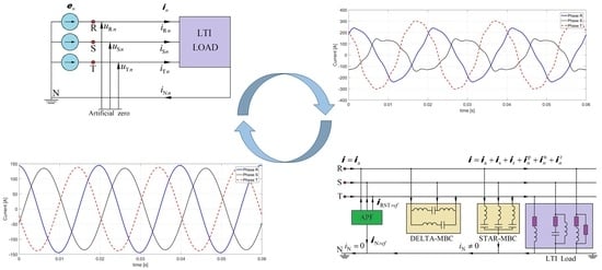
Figure 1 shows a three-phase four-wire system supplying an unbalanced linear time-invariant load (LTI).

Figure 1 shows the three-phase four-wire system supplying an unbalanced linear time-invariant load (LTI):

$$\mathit{u}\left(t\right)=\left[\begin{array}{c}{u}_{\mathrm{R}}\left(t\right)\\ u_{\mathrm{S}}\left(t\right)\\ u_{\mathrm{T}}\left(t\right)\end{array}\right]=\sqrt{2}\mathrm{Re}{\displaystyle \sum _{n\in N}\left[\begin{array}{c}{\mathit{U}}_{\mathrm{R}n}\\ {\mathit{U}}_{\mathrm{S}n}\\ {\mathit{U}}_{\mathrm{T}n}\end{array}\right]e^{jn{\omega }_{1}t}}=\sqrt{2}\mathrm{Re}{\displaystyle \sum _{n\in N}{\mathit{U}}_n{e}^{jn{\omega }_{1}t}},$$

(4)

where: ${\mathit{U}}_{\mathrm{R}n}$, ${\mathit{U}}_{\mathrm{S}n}$, ${\mathit{U}}_{\mathrm{T}n}$ are the nonsinusoidal complex RMS (CRMS) values of the voltages at the terminals R, S, and T of the load; ${\mathit{U}}_n$ is a three-phase vector of CRMS values of harmonics of phase voltages.

The vector of the currents of lines can be represented in the same way, namely:

$$\mathit{i}\left(t\right)=\left[\begin{array}{c}{i}_{\mathrm{R}}\left(t\right)\\ i_{\mathrm{S}}\left(t\right)\\ i_{\mathrm{T}}\left(t\right)\end{array}\right]=\sqrt{2}\mathrm{Re}{\displaystyle \sum _{n\in N}\left[\begin{array}{c}{\mathit{I}}_{\mathrm{R}n}\\ {\mathit{I}}_{\mathrm{S}n}\\ {\mathit{I}}_{\mathrm{T}n}\end{array}\right]e^{jn{\omega }_{1}t}}=\sqrt{2}\mathrm{Re}{\displaystyle \sum _{n\in N}{\mathit{I}}_n{e}^{jn{\omega }_{1}t}},$$

(5)

where: ${\mathit{I}}_{\mathrm{R}n}$, ${\mathit{I}}_{\mathrm{S}n}$, ${\mathit{I}}_{\mathrm{T}n}$ are the nonsinusoidal CRMS values of the currents in lines R, S, and T; ${\mathit{I}}_n$ is a three-phase vector of CRMS values of harmonics of line currents.

Considering the purpose of the article, only the final relationships necessary for understanding the next section will be presented in this section. Detailed information is presented in the authors’ publication [3].

Due to the currents’ physical components (CPC) theory, the current of an unbalanced LTI load supplied with an asymmetrical nonsinusoidal voltage [3] may have four components in total. The component of the current related to the permanent energy transmission from the source to the load is the active current ${\mathit{i}}_{\mathrm{a}}$, the waveform of which takes the form:

$${\mathit{i}}_{\mathrm{a}}=G_{\mathrm{e}}\mathit{u}={\displaystyle \sum _{n\in N}{\mathit{i}}_{\mathrm{a}n}}=\sqrt{2}\mathrm{Re}{\displaystyle \sum _{n\in N}{G}_{\mathrm{e}}{\mathit{U}}_n{e}^{jn{\omega }_{1}t}}=\sqrt{2}\mathrm{Re}{\displaystyle \sum _{n\in N}\left\{G_{\mathrm{e}}\left({\mathit{U}}_n^{\mathrm{p}}+{\mathit{U}}_n^{\mathrm{n}}+{\mathit{U}}_n^{\mathrm{z}}\right)e^{jn{\omega }_{1}t}\right\}}=\sqrt{2}\mathrm{Re}{\displaystyle \sum _{n\in N}\left\{G_{\mathrm{e}}\left({\mathbf{1}}^{\mathrm{p}}{\mathit{U}}_n^{\mathrm{p}}+{\mathbf{1}}^{\mathrm{n}}{\mathit{U}}_n^{\mathrm{n}}+{\mathbf{1}}^{\mathrm{z}}{\mathit{U}}_n^{\mathrm{z}}\right)e^{jn{\omega }_{1}t}\right\}},$$

(6)

where: ${\mathit{U}}_n^{\mathrm{p}}$, ${\mathit{U}}_n^{\mathrm{n}}$, ${\mathit{U}}_n^{\mathrm{z}}$ are the CRMS values of symmetrical voltage components accomplished from the Fortescue transformation; ${\mathbf{1}}^{\mathrm{p}}$, ${\mathbf{1}}^{\mathrm{n}}$, ${\mathbf{1}}^{\mathrm{z}}$ are the unit vectors of symmetrical components described by the Fortescue transformation; ${\mathit{U}}_n^{\mathrm{p}}$, ${\mathit{U}}_n^{\mathrm{n}}$, ${\mathit{U}}_n^{\mathrm{z}}$ are the vectors of the CRMS values of symmetrical voltage components accomplished from the Fortescue transformation.

The three-phase RMS value of an active current is associated to the equivalent conductance of the entire system $G_{\mathrm{e}}$ and to the three-phase RMS value of the supply voltage $‖\mathit{u}‖$:

$$‖{\mathit{i}}_{\mathrm{a}}‖=G_{\mathrm{e}}‖\mathit{u}‖=\frac{P}{‖\mathit{u}‖},$$

(7)

The component of the current associated with the presence of the difference between the equivalent conductance of the entire system $G_{\mathrm{e}}$ and the equivalent conductance of individual harmonics $G_{\mathrm{b}n}$ is the scattered current ${\mathit{i}}_{\mathrm{s}}$, the waveform of which can be presented as follows:

$$\begin{array}{l}{\mathit{i}}_{\mathrm{s}}={\displaystyle \sum _{n\in N}{\mathit{i}}_{\mathrm{s}n}}=\sqrt{2}\mathrm{Re}{\displaystyle \sum _{n\in N}\left\{\left(G_{\mathrm{b}n}-G_{\mathrm{e}}\right){\mathit{U}}_n{e}^{jn{\omega }_{1}t}\right\}}=\sqrt{2}\mathrm{Re}{\displaystyle \sum _{n\in N}\left\{\left(G_{\mathrm{b}n}-G_{\mathrm{e}}\right)\left({\mathit{U}}_n^{\mathrm{p}}+{\mathit{U}}_n^{\mathrm{n}}+{\mathit{U}}_n^{\mathrm{z}}\right)e^{jn{\omega }_{1}t}\right\}}\\ =\sqrt{2}\mathrm{Re}{\displaystyle \sum _{n\in N}\left\{\left(G_{\mathrm{b}n}-G_{\mathrm{e}}\right)\left({\mathbf{1}}^{\mathrm{p}}{\mathit{U}}_n^{\mathrm{p}}+{\mathbf{1}}^{\mathrm{n}}{\mathit{U}}_n^{\mathrm{n}}+{\mathbf{1}}^{\mathrm{z}}{\mathit{U}}_n^{\mathrm{z}}\right)e^{jn{\omega }_{1}t}\right\}}\end{array}$$

(8)

The three-phase RMS value of the scattered current $‖{\mathit{i}}_{\mathrm{s}}‖$ is calculated from the relationship:

$$‖{\mathit{i}}_{\mathrm{s}}‖=\sqrt{{\displaystyle \sum _{n\in N}\left[{\left(G_{\mathrm{b}n}-G_{\mathrm{e}}\right)}^2{‖{\mathit{u}}_n‖}^2\right]}},$$

(9)

The component of the current associated with the shift between the voltage waveform and the current waveform for individual harmonics and related to the equivalent parameter of the circuit in the form of equivalent susceptance $B_{\mathrm{b}n}$ is the reactive current ${\mathit{i}}_{\mathrm{r}}$, and its waveform is described as follows:

$${\mathit{i}}_{\mathrm{r}}={\displaystyle \sum _{n\in N}{\mathit{i}}_{\mathrm{r}n}}=\sqrt{2}\mathrm{Re}{\displaystyle \sum _{n\in N}\left\{j{B}_{\mathrm{b}n}{\mathit{U}}_n{e}^{jn{\omega }_{1}t}\right\}}=\sqrt{2}\mathrm{Re}{\displaystyle \sum _{n\in N}\left\{j{B}_{\mathrm{b}n}\left({\mathit{U}}_n^{\mathrm{p}}+{\mathit{U}}_n^{\mathrm{n}}+{\mathit{U}}_n^{\mathrm{z}}\right)e^{jn{\omega }_{1}t}\right\}}=\sqrt{2}\mathrm{Re}{\displaystyle \sum _{n\in N}\left\{j{B}_{\mathrm{b}n}\left({\mathbf{1}}^{\mathrm{p}}{\mathit{U}}_n^{\mathrm{p}}+{\mathbf{1}}^{\mathrm{n}}{\mathit{U}}_n^{\mathrm{n}}+{\mathbf{1}}^{\mathrm{z}}{\mathit{U}}_n^{\mathrm{z}}\right)e^{jn{\omega }_{1}t}\right\}},$$

(10)

The three-phase RMS value of the reactive current $‖{\mathit{i}}_{\mathrm{r}}‖$ is equal:

$$‖{\mathit{i}}_{\mathrm{r}}‖=\sqrt{{\displaystyle \sum _{n\in N}\left[{\left(B_{\mathrm{b}n}\right)}^2{‖{\mathit{u}}_n‖}^2\right]}},$$

(11)

where: $‖{\mathit{u}}_n‖$ is the three-phase RMS value of the voltage of the respective harmonic.

In the system, as a result of imbalanced of a load, there is also a fourth component of the current, called the unbalance current ${\mathit{i}}_{\mathrm{u}}$. The waveform of the unbalanced current is resulted by subtracting from the waveform of the total current $\mathit{i}$ three components in the form of active current ${\mathit{i}}_{\mathrm{a}}$, reactive current ${\mathit{i}}_{\mathrm{r}}$, and scattered current ${\mathit{i}}_{\mathrm{s}}$:

$$\begin{array}{cc}\hfill & {\mathit{i}}_{\mathrm{u}}={\displaystyle \sum _{n\in N}}{\mathit{i}}_{\mathrm{u}n}=\sqrt{2}\mathrm{Re}{\displaystyle \sum _{n\in N}}{\mathit{I}}_{\mathrm{u}n}{e}^{jn{\omega }_{1}t}=\sqrt{2}\mathrm{Re}{\displaystyle \sum _{n\in N}}\left\{\left({\mathit{I}}_n-{\mathit{I}}_{\mathrm{b}n}\right)e^{jn{\omega }_{1}t}\right\}\hfill \\ \hfill & =\sqrt{2}\mathrm{Re}{\displaystyle \sum _{n\in N}}\left\{\left({\mathit{I}}_n-{\mathit{Y}}_{\mathrm{b}n}{\mathit{U}}_n\right)e^{jn{\omega }_{1}t}\right\}=\sqrt{2}\mathrm{Re}{\displaystyle \sum _{n\in N}}\left\{\left({\mathit{I}}_n-\left(G_{\mathrm{e}}+\left(G_{\mathrm{b}n}-G_{\mathrm{e}}\right)+j{B}_{\mathrm{b}n}\right){\mathit{U}}_n\right)e^{jn{\omega }_{1}t}\right\}\hspace{1em}\hspace{1em}\hspace{1em}\hspace{1em} ,\hfill \\ \hfill & =\sqrt{2}\mathrm{Re}{\displaystyle \sum _{n\in N}}\left\{\left(\left({\mathit{I}}_n-{\mathit{I}}_{\mathrm{b}n}\right)\left({\mathbf{1}}^{\mathrm{p}}{\mathit{U}}_n^{\mathrm{p}}+{\mathbf{1}}^{\mathrm{n}}{\mathit{U}}_n^{\mathrm{n}}+{\mathbf{1}}^{\mathrm{z}}{\mathit{U}}_n^{\mathrm{z}}\right)\right)e^{jn{\omega }_{1}t}\right\}=\sqrt{2}\mathrm{Re}{\displaystyle \sum _{n\in N}}\left\{\left(\left({\mathit{I}}_n-{\mathit{I}}_{\mathrm{b}n}\right)\left({\mathit{U}}_n^{\mathrm{p}}+{\mathit{U}}_n^{\mathrm{n}}+{\mathit{U}}_n^{\mathrm{z}}\right)\right)\right\}{e}^{jn{\omega }_{1}t}\hfill \end{array}$$

(12)

where ${\mathit{I}}_{\mathrm{b}n}={\mathit{Y}}_{\mathrm{b}n}{\mathit{U}}_n$ is the vector of line currents consequent from the active and reactive powers of respective harmonics.

The three-phase RMS value of the unbalanced current $‖{\mathit{i}}_{\mathrm{u}}‖$ is:

$$‖{\mathit{i}}_{\mathrm{u}}‖=\sqrt{{‖\mathit{i}‖}^2-\left({‖{\mathit{i}}_{\mathrm{a}}‖}^2+{‖{\mathit{i}}_{\mathrm{r}}‖}^2+{‖{\mathit{i}}_{\mathrm{s}}‖}^2\right)},$$

(13)

Additionally, the unbalanced current can be divided into three symmetrical components of the appropriate order [3,4,5]. The first component of the unbalanced current ${\mathit{i}}_{\mathrm{u}}$ is the unbalanced current of the positive sequence ${\mathit{i}}_{\mathrm{u}}^{\mathrm{p}}$, which is related to the voltage asymmetry dependent admittance ${\mathit{Y}}_{\mathrm{d}n}$, the generalized unbalanced admittance of the positive sequence ${\mathit{Y}}_n^{\mathrm{p}}$, the generalized unbalanced admittance of the negative sequence ${\mathit{Y}}_n^{\mathrm{n}}$, and the generalized unbalanced admittance of the zero sequence ${\mathit{Y}}_n^{\mathrm{z}}$:

$${\mathit{i}}_{\mathrm{u}}^{\mathrm{p}}={\displaystyle \sum _{n\in N}{\mathit{i}}_{\mathrm{u}n}^{\mathrm{p}}}=\sqrt{2}\mathrm{Re}\left\{{\displaystyle \sum _{n\in N}{\mathit{I}}_{\mathrm{u}n}^{\mathrm{p}}{e}^{jn{\omega }_{1}t}}\right\}=\sqrt{2}\mathrm{Re}{\displaystyle \sum _{n\in N}\left\{{\mathbf{1}}^{\mathrm{p}}\left({\mathit{Y}}_{\mathrm{d}n}{\mathit{U}}_n^{\mathrm{p}}+{\mathit{Y}}_n^{\mathrm{p}}{\mathit{U}}_n^{\mathrm{p}}+{\mathit{Y}}_n^{\mathrm{z}}{\mathit{U}}_n^{\mathrm{n}}+{\mathit{Y}}_n^{\mathrm{n}}{\mathit{U}}_n^{\mathrm{z}}\right)e^{jn{\omega }_{1}t}\right\}},$$

(14)

The three-phase RMS value of the unbalanced current of the positive sequence is equal:

$$‖{\mathit{i}}_{\mathrm{u}}^{\mathrm{p}}‖=\sqrt{3\cdot {\displaystyle \sum _{n\in N}{\left|{\mathit{Y}}_{\mathrm{d}n}{\mathit{U}}_n^{\mathrm{p}}+{\mathit{Y}}_n^{\mathrm{p}}{\mathit{U}}_n^{\mathrm{p}}+{\mathit{Y}}_n^{\mathrm{z}}{\mathit{U}}_n^{\mathrm{n}}+{\mathit{Y}}_n^{\mathrm{n}}{\mathit{U}}_n^{\mathrm{z}}\right|}^2}},$$

(15)

The unbalanced current of the negative sequence ${\mathit{i}}_{\mathrm{u}}^{\mathrm{n}}$ can be determined analogically, the waveform of which can be described by the relationship:

$${\mathit{i}}_{\mathrm{u}}^{\mathrm{n}}={\displaystyle \sum _{n\in N}{\mathit{i}}_{\mathrm{u}n}^{\mathrm{n}}}=\sqrt{2}\mathrm{Re}\left\{{\displaystyle \sum _{n\in N}{\mathit{I}}_{\mathrm{u}n}^{\mathrm{n}}{e}^{jn{\omega }_{1}t}}\right\}=\sqrt{2}\mathrm{Re}{\displaystyle \sum _{n\in N}\left\{{\mathbf{1}}^{\mathrm{n}}\left({\mathit{Y}}_{\mathrm{d}n}{\mathit{U}}_n^{\mathrm{n}}+{\mathit{Y}}_n^{\mathrm{n}}{\mathit{U}}_n^{\mathrm{p}}+{\mathit{Y}}_n^{\mathrm{p}}{\mathit{U}}_n^{\mathrm{n}}+{\mathit{Y}}_n^{\mathrm{z}}{\mathit{U}}_n^{\mathrm{z}}\right)e^{jn{\omega }_{1}t}\right\}},$$

(16)

The three-phase RMS value of the unbalanced current of the negative sequence is equal:

$$‖{\mathit{i}}_{\mathrm{u}}^{\mathrm{n}}‖=\sqrt{3\cdot {\displaystyle \sum _{n\in N}{\left|{\mathit{Y}}_{\mathrm{d}n}{\mathit{U}}_n^{\mathrm{n}}+{\mathit{Y}}_n^{\mathrm{n}}{\mathit{U}}_n^{\mathrm{p}}+{\mathit{Y}}_n^{\mathrm{p}}{\mathit{U}}_n^{\mathrm{n}}+{\mathit{Y}}_n^{\mathrm{z}}{\mathit{U}}_n^{\mathrm{z}}\right|}^2}},$$

(17)

The last component is the unbalanced current of the zero sequence ${\mathit{i}}_{\mathrm{u}}^{\mathrm{z}}$. The waveform of this current is:

$${\mathit{i}}_{\mathrm{u}}^{\mathrm{z}}={\displaystyle \sum _{n\in N}{\mathit{i}}_{\mathrm{u}n}^{\mathrm{z}}}=\sqrt{2}\mathrm{Re}{\displaystyle \sum _{n\in N}\left\{{\mathit{I}}_{\mathrm{u}n}^{\mathrm{z}}{e}^{jn{\omega }_{1}t}\right\}}=\sqrt{2}\mathrm{Re}{\displaystyle \sum _{n\in N}\left\{{\mathbf{1}}^{\mathrm{z}}\left({\mathit{Y}}_{\mathrm{d}n}{\mathit{U}}_n^{\mathrm{z}}+{\mathit{Y}}_n^{\mathrm{z}}{\mathit{U}}_n^{\mathrm{p}}+{\mathit{Y}}_n^{\mathrm{n}}{\mathit{U}}_n^{\mathrm{n}}+{\mathit{Y}}_n^{\mathrm{p}}{\mathit{U}}_n^{\mathrm{z}}\right)e^{jn{\omega }_{1}t}\right\}},$$

(18)

The three-phase RMS value of the unbalanced current of the zero sequence is equal:

$$‖{\mathit{i}}_{\mathrm{u}}^{\mathrm{z}}‖=\sqrt{3\cdot {\displaystyle \sum _{n\in N}{\left|{\mathit{Y}}_{\mathrm{d}n}{\mathit{U}}_n^{\mathrm{z}}+{\mathit{Y}}_n^{\mathrm{z}}{\mathit{U}}_n^{\mathrm{p}}+{\mathit{Y}}_n^{\mathrm{n}}{\mathit{U}}_n^{\mathrm{n}}+{\mathit{Y}}_n^{\mathrm{p}}{\mathit{U}}_n^{\mathrm{z}}\right|}^2}},$$

(19)

In relation to the fact that all components are mutually orthogonal [3], the three-phase RMS value of the load’s current, according to currents’ physical components theory, is:

$${‖\mathit{i}‖}^2={‖{\mathit{i}}_{\mathrm{a}}‖}^2+{‖{\mathit{i}}_{\mathrm{s}}‖}^2+{‖{\mathit{i}}_{\mathrm{r}}‖}^2+{‖{\mathit{i}}_{\mathrm{u}}^{\mathrm{p}}‖}^2+{‖{\mathit{i}}_{\mathrm{u}}^{\mathrm{n}}‖}^2+{‖{\mathit{i}}_{\mathrm{u}}^{\mathrm{z}}‖}^2,$$

(20)

The respective powers are obtained by multiplying the three-phase RMS value of the supply voltage and the three-phase RMS values of the individual components of the load current (7), (9), (11), (12), (17), and (19):

$$S=\sqrt{P^2+Q^2+D_{\mathrm{s}}^2+D_{\mathrm{u}}^{\mathrm{p}2}+D_{\mathrm{u}}^{\mathrm{n}2}+D_{\mathrm{u}}^{\mathrm{z}2}},$$

(21)

The power factor $\lambda$ can be expressed in terms of the powers’ components or the currents’ components:

$$\lambda =\frac{P}{S}=\frac{P}{\sqrt{P^2+Q^2+D_{\mathrm{s}}^2+D_{\mathrm{u}}^{\mathrm{p}\hspace{0.17em}2}+D_{\mathrm{u}}^{\mathrm{n}\hspace{0.17em}2}+D_{\mathrm{u}}^{\mathrm{z}\hspace{0.17em}2}}}=\frac{‖{\mathit{i}}_{\mathrm{a}}‖}{‖\mathit{i}‖}=\frac{‖{\mathit{i}}_{\mathrm{a}}‖}{\sqrt{{‖{\mathit{i}}_{\mathrm{a}}‖}^2+{‖{\mathit{i}}_{\mathrm{r}}‖}^2+{‖{\mathit{i}}_{\mathrm{s}}‖}^2+{‖{\mathit{i}}_{\mathrm{u}}^{\mathrm{p}}‖}^2+{‖{\mathit{i}}_{\mathrm{u}}^{\mathrm{n}}‖}^2+{‖{\mathit{i}}_{\mathrm{u}}^{\mathrm{z}}‖}^2}},$$

(22)

As can be seen, the power factor $\lambda$ consists of six powers or currents which, apart from the active power P or the three-phase RMS value of the active current, are lower than its value. It should also be mentioned that in systems with nonsinusoidal waveforms, the power factor $\lambda$ will not reach the value equal to 1, as long as there is the scattered current in the considered system.

3. Theoretical Illustration—Currents’ Components

For theoretical illustration, the system shown in Figure 2 has been prepared. This is a three-phase four-wire system supplied with an asymmetrical nonsinusoidal voltage. The load is unbalanced and is an LTI load type. In the voltage source, in addition to the fundamental harmonic with a frequency of 50 Hz, harmonics 3rd, 5th, and 7th are also presence.

The values of resistance as well as capacitive and inductive reactance for the fundamental harmonic, shown in Figure 2, are presented in

Table 1. List of phase impedances with division of resistance, inductive, and capacitive reactance values.

Line	Resistance R [Ω]	Inductive Reactance XL [Ω]	Capacitive reactance XC [Ω]
R	1	1	-
S	2	1.5	2
T	R1 = 0.5, R2 = 5	1	-

.

Table 2. List of the values of the phase voltages and the values of the line currents.

Harmonic Order	Phase R	Phase S	Phase T
	${\mathit{U}}_{\mathit{n}} \left[\mathbf{V}\right]$
1st	$230e^{j{5}^{\circ }}$	$215e^{-j{110}^{\circ }}$	$220e^{j{99}^{\circ }}$
3rd	$20e^{j{0}^{\circ }}$	$33e^{j{10}^{\circ }}$	$30e^{-j{20}^{\circ }}$
5th	$40e^{-j{6}^{\circ }}$	$20e^{j{114}^{\circ }}$	$27e^{-j{133}^{\circ }}$
7th	$19e^{j{7}^{\circ }}$	$10e^{-j{100}^{\circ }}$	$30e^{j{124}^{\circ }}$
	${\mathit{I}}_n$ [A]
1st	$162.64e^{-j{40}^{\circ }}$	$104.47e^{-j{169}^{\circ }}$	$220e^{j{45.9}^{\circ }}$
3rd	$6.33e^{-j{71.6}^{\circ }}$	$15.04e^{j{0.9}^{\circ }}$	$12.36e^{-j{71.9}^{\circ }}$
5th	$7.85e^{-j{84.7}^{\circ }}$	$9.64e^{j{109.6}^{\circ }}$	$7.99e^{-j{175}^{\circ }}$
7th	$2.69e^{-j{74.9}^{\circ }}$	$4.91e^{-j{103}^{\circ }}$	$7.61e^{j{89.9}^{\circ }}$

presents the values of the voltages harmonics and the values of the harmonics of the line currents of the load.

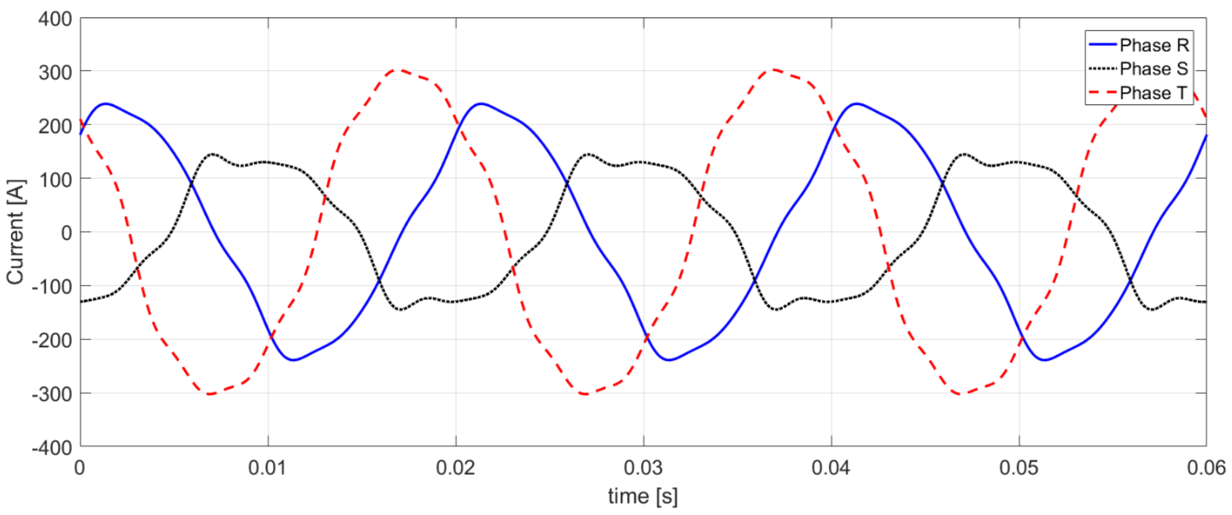
Figure 3 shows the three-phase voltage waveform at the terminals of the analyzed load, and the three-phase waveform of the line current is shown in Figure 4.

The equivalent parameters of the load presented in Figure 1 (in accordance with CPC Theory [3]) are listed in

Table 3. List of the values of the individuals admittances.

Parameter [S]	Harmonic Order
	1st	3rd	5th	7th
$G_{\mathrm{e}}$	$0.445$
$G_{\mathrm{b}n}$	$0.454$	$0.318$	$0.152$	$0.180$
$B_{\mathrm{b}n}$	$-0.572$	$-0.205$	$-0.171$	$-0.133$
${\mathit{Y}}_{\mathrm{d}n}$	$4.475\cdot {10}^{-3}{e}^{j{178.8}^{\circ }}$	$0.056e^{-j{151.6}^{\circ }}$	$0.099e^{j{16.8}^{\circ }}$	$0.067e^{j{27.1}^{\circ }}$
${\mathit{Y}}_n^{\mathrm{p}}$	-	-	-	-
${\mathit{Y}}_n^{\mathrm{n}}$	$0.107e^{-j{142.8}^{\circ }}$	$0.158e^{j{171.8}^{\circ }}$	$0.159e^{j{161.5}^{\circ }}$	$0.157e^{j{156.7}^{\circ }}$
${\mathit{Y}}_n^{\mathrm{z}}$	$0.193e^{j{45.3}^{\circ }}$	$0.091e^{-j{97.1}^{\circ }}$	$0.116e^{-j{119.9}^{\circ }}$	$0.125e^{-j{127.5}^{\circ }}$

.

Extensive information why the generalized unbalanced admittance of the positive sequence is always 0 is presented in [3].

Based on the information included in Table 2, the three-phase RMS values of the supply voltages are 392.43 V, and the three-phase RMS values of the currents of the line are 294.09 A.

Table 4. List of the values of the currents’ components.

Current [A]	Harmonic Order				Total Value [A]
	1st	3rd	5th	7th
$‖{\mathit{i}}_{\mathrm{a}}‖$	$170.75$	$21.73$	$23.22$	$16.40$	$174.46$
$‖{\mathit{i}}_{\mathrm{s}}‖$	$3.81$	$6.21$	$15.30$	$9.75$	$19.55$
$‖{\mathit{i}}_{\mathrm{r}}‖$	$219.82$	$10.04$	$8.94$	$4.91$	$220.29$
$‖{\mathit{i}}_{\mathrm{u}}^{\mathrm{p}}‖$	$18.55$	$6.73$	$4.68$	$0.83$	$20.30$
$‖{\mathit{i}}_{\mathrm{u}}^{\mathrm{n}}‖$	$28.08$	$5.20$	$2.24$	$3.86$	$28.91$
$‖{\mathit{i}}_{\mathrm{u}}^{\mathrm{z}}‖$	$76.42$	$2.23$	$6.98$	$2.29$	$76.81$
$‖\mathit{i}‖$	$292.86$	$20.47$	$14.78$	$9.45$	$294.09$

presents the three-phase RMS values of currents’ components for appropriate harmonics described in CPC Theory (7), (9), (11), (15), (17), and (19). In Table 4 are also included the total three-phase values for specific currents’ components and the total value of the three-phase current (20).

Based on (7), (9), (11), (15), (17), and (19) and using the already known three-phase RMS values of appropriate components, the power factor $\lambda$ (22) is 0.593.

As can be seen from the value of the power factor $\lambda$, it follows that the considered system should be subjected to compensation and balancing. The balancing compensation can be performed passively by using reactance elements in the form of chokes and/or capacitors. Compensation and balancing can also be carried out actively using an active power filter (APF). It is also possible to use a hybrid system in the form of a designed balancing compensator made of passive elements and an active part in the form of an APF. The third solution is a very often used compromise between the accuracy of compensation and symmetrization and the economic justification for improving the quality of electricity.

4. The Compensator Minimizes the Reactive Current and the Unbalanced Current on the Basis of the Currents’ Physical Components Theory in 3-p 4-w Systems

Due to the number of elements in one branch, the most advantageous condition is that such a branch has only one reactance element. Unfortunately, in the real conditions of the power system, if the compensator branch has a capacitive impedance, it can very often resonate with the system for higher harmonics. To prevent such a phenomenon, the compensator branch should be purely inductive or it should be connected in series with the capacitor, forming the LC branch [6,43,44,45,46].

The vector of the complex RMS values of nonsinusoidal voltages in the branches of balancing compensators takes the form:

$${\mathit{U}}_{\mathrm{n}}={\left[\begin{array}{cccccc}{\mathit{U}}_{\mathrm{RS}n}& {\mathit{U}}_{\mathrm{ST}n}& {\mathit{U}}_{\mathrm{TR}n}& {\mathit{U}}_{\mathrm{R}n}& {\mathit{U}}_{\mathrm{S}n}& {\mathit{U}}_{\mathrm{T}n}\end{array}\right]}^{\mathrm{T}},$$

(23)

where the nonsinusoidal phase-to-phase voltages are described in [46,47], and the nonsinusoidal phase voltages by Equation (4)

The vector of the branch currents of an ideal balancing compensator can be represented as:

$${\mathit{j}}_{\mathrm{T}}=\sqrt{2}\mathrm{Re}{\displaystyle \sum _{n\in N}j{\mathit{T}}_n{\mathit{U}}_n{e}^{jn{\omega }_{1}t}},$$

(24)

where the vector ${\mathit{T}}_n$ is:

$${\mathit{T}}_n=\left[\begin{array}{cccccc}{T}_{\mathrm{RS}n}& 0& 0& 0& 0& 0\\ 0& T_{\mathrm{ST}n}& 0& 0& 0& 0\\ 0& 0& T_{\mathrm{TR}n}& 0& 0& 0\\ 0& 0& 0& T_{\mathrm{R}n}& 0& 0\\ 0& 0& 0& 0& T_{\mathrm{S}n}& 0\\ 0& 0& 0& 0& 0& T_{\mathrm{T}n}\end{array}\right],$$

(25)

The vector ${\mathit{T}}_n$ consists of two components relating to ideal balancing compensators. The elements $T_{\mathrm{ST}n}$, $T_{\mathrm{RS}n}$, $T_{\mathrm{TR}n}$ refer to the value of the ideal balancing compensator (the index “n” means the order of harmonics) in the delta structure. So they are phase-to-phase susceptances. The elements of the $T_{\mathrm{R}n}$, $T_{\mathrm{S}n}$, $T_{\mathrm{T}n}$ refer to the value of the ideal balancing compensator in the star structure. So they are phase-to-neutral susceptances.

For the minimizing balancing compensator (MBC), the reactive current, and the unbalanced currents, the vector of the branch currents can be represented as follows:

$${\mathit{j}}_{\mathrm{D}}=\sqrt{2}\mathrm{Re}{\displaystyle \sum _{n\in N}j{\mathit{D}}_n{\mathit{U}}_n{e}^{jn{\omega }_{1}t}},$$

(26)

where the vector ${\mathit{D}}_n$ is:

$${\mathit{D}}_n=\left[\begin{array}{cccccc}{D}_{\mathrm{RS}n}& 0& 0& 0& 0& 0\\ 0& D_{\mathrm{ST}n}& 0& 0& 0& 0\\ 0& 0& D_{\mathrm{TR}n}& 0& 0& 0\\ 0& 0& 0& D_{\mathrm{R}n}& 0& 0\\ 0& 0& 0& 0& D_{\mathrm{S}n}& 0\\ 0& 0& 0& 0& 0& D_{\mathrm{T}n}\end{array}\right],$$

(27)

The vector ${\mathit{D}}_n$, identical to the vector ${\mathit{T}}_n$, consists of two compensators of different structures. The main difference between the elements in both vectors is the ideality of the constituent elements. The susceptances $D_{\mathrm{RS}n}$, $D_{\mathrm{ST}n}$, $D_{\mathrm{TR}n}$ in the delta system are designed to minimize the value of unbalanced currents of the negative and positive sequences, but not for ideal compensation. The same is the case with susceptances $D_{\mathrm{R}n}$, $D_{\mathrm{S}n}$, $D_{\mathrm{T}n}$. The selection of the parameters of these susceptances is to contribute to the reduction of reactive current and the unbalanced current of the zero sequence. In order to be able to optimally minimize the reactive current and the unbalanced current, the minimum distance should be determined for these two vectors.

The distance of the ${\mathit{j}}_{\mathrm{T}}$ and ${\mathit{j}}_{\mathrm{D}}$ vectors can be defined as the RMS value of the difference of their currents, namely:

$$d=‖{\mathit{j}}_{\mathrm{T}}-{\mathit{j}}_{\mathrm{D}}‖=‖\mathsf{\Delta }\mathit{j}‖,$$

(28)

Two compensators with the susceptances $D_{\mathrm{RS}n},\hspace{0.17em}\hspace{0.17em}{D}_{\mathrm{ST}n},\hspace{0.17em}\hspace{0.17em}{D}_{\mathrm{TR}n}$ and $D_{\mathrm{R}n},\hspace{0.17em}\hspace{0.17em}{D}_{\mathrm{S}n},\hspace{0.17em}\hspace{0.17em}{D}_{\mathrm{T}n}$, compensate and balance the unbalanced currents of the positive and negative sequences (the balancing compensator in delta structure) and the reactive current and the unbalanced current of the zero sequence (the balancing compensator in star structure), respectively. If the RMS value of the difference of hypothetical currents, ideal balancing compensators, and the minimizing balancing compensators built of at most two-elements LC, equal to:

$$\mathsf{\Delta }\mathit{j}=\sqrt{2}\mathrm{Re}{\displaystyle \sum _{n\in N}\left({\mathit{T}}_n-{\mathit{D}}_n\right)}\hspace{0.17em}{\mathit{U}}_n{e}^{jn{\omega }_{1}t}=\sqrt{2}\mathrm{Re}{\displaystyle \sum _{n\in N}\mathsf{\Delta }{\mathit{J}}_n{e}^{jn{\omega }_{1}t}},$$

(29)

is as small as possible, then the square of the RMS value of this current, otherwise the square of the distance of the currents ${\mathit{j}}_{\mathrm{T}}$ and ${\mathit{j}}_{\mathrm{D}}$ is equal to:

$$\begin{array}{l}{d}^2={‖\mathsf{\Delta }\mathit{j}‖}^2=\mathrm{Re}{\displaystyle \sum _{n\in N}\mathsf{\Delta }{\mathit{J}}_n^{\mathrm{T}}\cdot }\hspace{0.17em}\mathsf{\Delta }{\mathit{J}}_n^{*}={\displaystyle \sum _{n\in N}\left(\mathsf{\Delta }{J}_{\mathrm{RS}n}^2+\mathsf{\Delta }{J}_{\mathrm{ST}n}^2+\mathsf{\Delta }{J}_{\mathrm{TR}n}^2+\mathsf{\Delta }{J}_{\mathrm{R}n}^2+\mathsf{\Delta }{J}_{\mathrm{S}n}^2+\mathsf{\Delta }{J}_{\mathrm{T}n}^2\right)}\\ ={\displaystyle \sum _{n\in N}\left[{\left(T_{\mathrm{RS}n}-D_{\mathrm{RS}n}\right)}^2{U}_{\mathrm{RS}n}^2+{\left(T_{\mathrm{ST}n}-D_{\mathrm{ST}n}\right)}^2{U}_{\mathrm{ST}n}^2+{\left(T_{\mathrm{TR}n}-D_{\mathrm{TR}n}\right)}^2{U}_{\mathrm{TR}n}^2\right.}+\left.{\left(T_{\mathrm{R}n}-D_{\mathrm{R}n}\right)}^2{U}_{\mathrm{R}n}^2+{\left(T_{\mathrm{S}n}-D_{\mathrm{S}n}\right)}^2{U}_{\mathrm{S}n}^2+{\left(T_{\mathrm{T}n}-D_{\mathrm{T}n}\right)}^2{U}_{\mathrm{T}n}^2\right]\end{array}$$

(30)

The square of the currents distances ${\mathit{j}}_{\mathrm{T}}$ and ${\mathit{j}}_{\mathrm{D}}$ is therefore the sum of three nonnegative, mutually separate terms for each of the balancing compensator structures, the general form of which can be written as follows:

$$d=‖{\mathit{j}}_{\mathrm{T}}-{\mathit{j}}_{\mathrm{D}}‖=\sqrt{{\displaystyle \sum _{n\in N}\mathsf{\Delta }{\mathit{J}}_n^{\mathrm{T}}\cdot }\hspace{0.17em}\mathsf{\Delta }{\mathit{J}}_n^{*}}=\sqrt{{\displaystyle \sum _{n\in N}{\displaystyle \sum _{k\in K}{\left(T_{kn}-D_{kn}\right)}^2{U}_{kn}^2}}},$$

(31)

where $k$ is a symbol in the set $K=\left\{\mathrm{RS},\hspace{0.17em}\hspace{0.17em}\mathrm{ST},\hspace{0.17em}\hspace{0.17em}\mathrm{TR},\hspace{0.17em}\hspace{0.17em}\mathrm{R},\hspace{0.17em}\hspace{0.17em}\mathrm{S},\hspace{0.17em}\hspace{0.17em}\mathrm{T}\right\}$.

On the grounds of that the order of summing the harmonic orders $n$ and the branch indexes $k$ can be different, the distance $d$ could be expressed as follows:

$$d=\sqrt{{\displaystyle \sum _{n\in N}{\displaystyle \sum _{k\in K}{\left(T_{kn}-D_{kn}\right)}^2{U}_{kn}^2}}}=\sqrt{{\displaystyle \sum _{k\in K}{d}_k^2}},$$

(32)

As can be seen, the values under the square root will be nonnegative numbers, so it is not possible for the values to eliminate.

The distance d is minimal when the individual distances $d_k$ for individual branches of the balancing compensators are also minimal, namely:

$${\displaystyle \sum _{n\in N}{\left(T_{kn}-D_{kn}\right)}^2{U}_{kn}^2=\hspace{0.17em}\mathrm{minimum}},$$

(33)

It is known that the RMS value of the fundamental voltage harmonic, whether phase-to-phase or phase, is much higher than the RMS value of any other harmonic [6,43,44,45,46]. Consequently, if in individual branches of one of the two compensators no resonance appears in the nearby of the harmonic frequency of the supply voltage, then the dominant component in the distance $d$ of the ${\mathit{j}}_{\mathrm{T}}$ and ${\mathit{j}}_{\mathrm{D}}$ vectors is the difference in susceptance between the ideal and minimizing compensator in a given branch for the fundamental frequency, i.e.,: T_XY1—D_XY1 or T_X1—D_X1. This assumption determines the choice of susceptance for the fundamental frequency D_XY1 or D_X1, namely, their signs must be the same as those of T_XY1 or T_X1 susceptance.

It was assumed that if the susceptance of T_XY1 or T_X1 is negative, then the compensator with a delta structure between the T_XY terminals should have a branch with a choke, because its susceptance is also negative, or if the compensator with a star structure between the phase terminal and the neutral wire T_X should also have branch with a choke. The inductance of such a choke, regardless of whether it is connected between phases or phase and neutral wire, should minimize the value:

$${\displaystyle \sum _{n\in N}{\left(T_{kn}+\frac{1}{n {\omega }_1{L}_k}\right)}^2{U}_{kn}^2=\mathrm{minimum}},$$

(34)

If the line-to-line susceptance T_XY or the line susceptance T_X is positive, the compensator should have a capacitor in the branch, but it should be connected in series with the choke, so that for higher order harmonics this branch has an inductive character and positive for the fundamental frequency:

$$d_{k1}=\frac{{\omega }_1{C}_k}{1-{\omega }_1^2 L_k{C}_k},$$

(35)

This requires that the resonant frequency of such a branch be higher than the fundamental frequency, i.e.,:

$${\omega }_{\mathrm{r}}=\frac{1}{\sqrt{L_k{C}_k}},$$

(36)

The inductance and capacitance of such a branch should minimize the following expression:

$${\displaystyle \sum _{n\in N}{\left(T_{kn}-\frac{n{\omega }_1{C}_k}{1-n^2 {\omega }_1^2 L_k{C}_k}\right)}^2{U}_{kn}^2=\mathrm{minimum}},$$

(37)

The inductance $L_k$ satisfying Equation (34) can be found from the condition:

$$\frac{d}{d{L}_k}\left\{{\displaystyle \sum _{n\in N}{\left(T_{kn}+\frac{1}{n{\omega }_1 L_k}\right)}^2{U}_{kn}^2}\right\}=0,$$

(38)

By fulfilling the expression (38), i.e., by calculating the inductance of a given branch, we can treat it as the optimal inductance of that branch, therefore:

$$L_{k,\hspace{0.17em}\mathrm{opt}}=-\frac{{\displaystyle \sum _{n\in N}\frac{U_{kn}^2}{n^2}}}{{\omega }_1{\displaystyle \sum _{n\in N}\frac{T_{kn}{U}_{kn}^2}{n}}},$$

(39)

The left side of the expression (37) is a function of two variables, i.e., inductance $L_k$ and capacitance $C_k$. The inductance of $L_k$ is a continuously decreasing function, which means that there is no minimum for any finite value. Its choice depends on the person accomplishing the calculations [43,44,45]. After choosing the inductance, the capacitance $C_k$ can be calculated from formula (37). When looking for the minimum in expression (37), we have to fulfill the condition:

$$\frac{d}{d{C}_k}\left\{{\displaystyle \sum _{n\in N}{\left(T_{kn}-\frac{n{\omega }_1{C}_k}{1-n^2 {\omega }_1^2 L_k{C}_k}\right)}^2{U}_{kn}^2}\right\}=0,$$

(40)

The distance defined by the expression (40) for any branch has a minimum due to the optimal capacitance of the capacitor when:

$${\displaystyle \sum _{n\in N}\frac{n{T}_{kn}{U}_{kn}^2}{{\left(1-n^2 {\omega }_1^2 L_{k,\hspace{0.17em}\mathrm{opt}}{C}_{k,\hspace{0.17em}\mathrm{opt}}\right)}^2}-{\displaystyle \sum _{n\in N}\frac{n^2{\omega }_1{C}_{k,\hspace{0.17em}\mathrm{opt}}{U}_{kn}^2}{{\left(1-n^2 {\omega }_1^2 L_{k,\hspace{0.17em}\mathrm{opt}}{C}_{k,\hspace{0.17em}\mathrm{opt}}\right)}^3}=0}},$$

(41)

Considering the optimal capacity $C_{k,\hspace{0.17em}\mathrm{opt}}$ occurring in the dependence (41), this equation is an implicit equation. Therefore, calculating this capacity requires numerical methods, especially in an iterative process. The iterative formula for determining the optimal capacity takes the form:

$$C_{k,\hspace{0.17em}\hspace{0.17em}i+1}=\frac{{\displaystyle \sum _{n\in N}\frac{n{T}_{kn}{U}_{kn}^2}{{\left(1-n^2{\omega }_1^2{L}_{k,\hspace{0.17em}\mathrm{opt}}{C}_{k,\hspace{0.17em}\hspace{0.17em}i}\right)}^2}}}{{\omega }_1{\displaystyle \sum _{n\in N}\frac{n^2{U}_{kn}^2}{{\left(1-n^2{\omega }_1^2{L}_{k,\hspace{0.17em}\mathrm{opt}}{C}_{k,\hspace{0.17em}\hspace{0.17em}i}\right)}^3}}},$$

(42)

After the ith iteration, it will concur to obtain several capacities, which in the final stage of calculation should cause to the optimal capacity.

5. Theoretical Illustration—Symmetrization and Compensation of Currents’ Components and Minimalization of the Structure of Balancing Compensators

For the theoretical illustration of the minimizing balancing compensation, the system analyzed in Figure 2 was chosen. According to the information in Chapter 4, the minimization is primarily focused on incomplete balancing compensation of reactive current and the unbalanced current, as well as limiting the number of reactive elements to a maximum of two in one branch [6,43,44,45,46].

Based on Equation (36), the resonant frequency was chosen with the value ${\omega }_{\mathrm{r}}=1.07{\omega }_{\hspace{0.17em}1}$.

Table 5. List of the values of the reactive elements for the minimizing balancing compensators.

Structure	R		S		T
STAR-MBC	$C$[$\mathsf{\mu }\mathrm{F}$]	$L$[$\mathrm{mH}$]	$C$[$\mathsf{\mu }\mathrm{F}$]	$L$[$\mathrm{mH}$]	$C$[$\mathsf{\mu }\mathrm{F}$]	$L$[$\mathrm{mH}$]
	$95.21$	$92.75$	$203.91$	$43.38$	$402.29$	$21.93$
	RS		ST		TR
DELTA-MBC	$C$[$\mathsf{\mu }\mathrm{F}$]	$L$[$\mathrm{mH}$]	$C$[$\mathsf{\mu }\mathrm{F}$]	$L$[$\mathrm{mH}$]	$C$[$\mathsf{\mu }\mathrm{F}$]	$L$[$\mathrm{mH}$]
	$53.96$	$163.83$	$-$	$21.2$	$28.88$	$307.93$

presents the values of the reactance elements of the minimizing balancing compensators (MBC) with star (STAR-MBC) and delta (DELTA-MBC) structures, calculated on the basis of expressions (39) and (42). The required optimal capacity in each branch was estimated in the fifth iteration.

Figure 5 shows the analyzed system which connected the minimizing balancing compensators in both structures.

Table 6. List of the values of the three-phase currents’ components after the minimizing balancing compensation.

Current [A]	Harmonic Order				Total Value [A]
	1st	3rd	5th	7th
$‖{\mathit{i}}_{\mathrm{a}}‖$	$170.75$	$21.73$	$23.22$	$16.40$	$174.46$
$‖{\mathit{i}}_{\mathrm{s}}‖$	$3.81$	$6.21$	$15.30$	$9.75$	$19.55$
$‖{\mathit{i}}_{\mathrm{r}}‖$	$3.56$	$12.11$	$10.96$	$6.45$	$17.92$
$‖{\mathit{i}}_{\mathrm{u}}^{\mathrm{p}}‖$	$0.82$	$7.23$	$3.54$	$0.95$	$8.14$
$‖{\mathit{i}}_{\mathrm{u}}^{\mathrm{n}}‖$	$2.04$	$5.70$	$2.04$	$4.11$	$7.59$
$‖{\mathit{i}}_{\mathrm{u}}^{\mathrm{z}}‖$	$2.89$	$2.43$	$7.23$	$2.29$	$8.47$
$‖\mathit{i}‖$	$170.87$	$27.35$	$31.02$	$20.71$	$177.02$

presents the three-phase RMS values of the component currents, defined in the CPC theory, after the minimizing the balancing compensation shown in Figure 5.

As can be observed in Table 6, as a result of connecting the compensators MBC, the three-phase RMS currents for higher harmonics have increased. It is related to the purposeful inaccuracy of the inductive susceptances so that there is no resonance phenomenon between the MBC and the inductance of the power network. The increase in the three-phase RMS values of the component currents does not, however, result in the flow of a large amount of energy, because the amplitudes of the harmonic voltages are also relatively low in relation to the fundamental harmonic voltage.

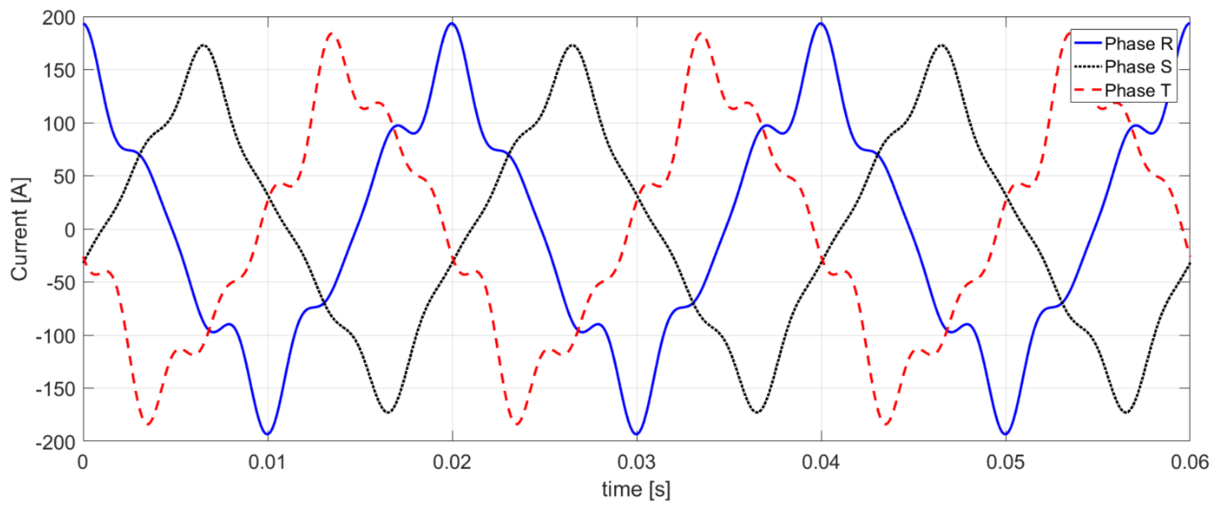
Figure 6 shows the waveform of line currents after the minimizing the balancing compensation.

Due to the use of the minimizing balancing compensation, the power factor $\lambda$ (22) increased to the value of 0.986.

This means that in systems with the scattered current associated with a change in conductance on the order of harmonics, it is not possible to obtain the power factor $\lambda$ equal to unity. For this to become, such a system should use power electronic elements, known as an active power filter.

6. CPC Theory—The Possibility of Using the Active Power Filter to Generate the Reference Current

The active power filter (APF) as a compensator for reactive power (reactive current) and unbalanced power (unbalanced current) has to be equipped with a measurement and identification system for the load’s parameters. Currents and voltages can be measured at the spot, where it will be operated without feedback, or where the feedback loop will be required. In the first case, the system will be investigated as a stable system, while in the second case, problems with stability may appear. The problem of stability must therefore be included in the APF control algorithm.

Stability is not investigated in this article. Essentially, the identification of the parameters of an unbalanced three-phase load, which is performed by measuring the currents and voltages at its terminals, is significant for compensation. The identification of the load has to be made on the basis of the knowledge of the current and voltage waveforms, and more precisely, the sequences of their discrete values, provided by the waveform sampling system and the analog-to-digital converter. When the sampled sequences are known, the complex RMS values of the supply voltage, load currents, and the current in the neutral conductor can be calculated, i.e.,: ${\mathit{U}}_{\mathrm{R}},\hspace{0.17em}\hspace{0.17em}{\mathit{U}}_{\mathrm{S}},\hspace{0.17em}\hspace{0.17em}{\mathit{U}}_{\mathrm{T}},\hspace{0.17em}\hspace{0.17em}{\mathit{I}}_{\mathrm{R}},\hspace{0.17em}\hspace{0.17em}{\mathit{I}}_{\mathrm{S}},\hspace{0.17em}\hspace{0.17em}{\mathit{I}}_{\mathrm{T}}$ and ${\mathit{I}}_{\mathrm{N}}$, which will be the resultant of the line currents. The most common method for this is the discrete Fourier transform (DFT) together with the fast Fourier transform (FFT) algorithm [9,16,48]. It is also possible to abbreviate the computational time by using the algorithm described in [49].

Before launching the capability of generating a reference current in an active power filter, the appropriate APF system should be chosen first. Among many available solutions [9,10,12,13,14,15,16,17,18,50,51,52], four-wire systems [10,15] should be used. The use of four-wire systems has the advantage over three-wire systems that in addition to injecting reference currents to compensate for the line currents i_R (t), i_S (t), and i_T (t), it is also possible to inject a reference current to compensate for the current in the neutral wire i_N (t). As it is known, the current in the neutral wire with non-linear loads or with unbalanced linear loads can reach very high values.

To obtain the reference current ${\mathrm{i}}_{\mathrm{RST}ref}\left(t\right)$ of an active power filter or a hybrid power filter (the active part of this filter), we use the system of equations:

$$i_{\mathrm{RST}ref}\left(t\right)=\left\{\begin{array}{c}{i}_{\mathrm{R}ref}\left(t\right)=-\sqrt{2}\mathrm{Re}\left\{{\displaystyle \sum _{n=1}^N}{i}_{\mathrm{rR}n}\left(t\right)+{\displaystyle \sum _{n=1}^N}{i}_{\mathrm{sR}n}\left(t\right)+{\displaystyle \sum _{n=1}^N}{i}_{\mathrm{uR}n}^{\mathrm{p}}\left(t\right)+{\displaystyle \sum _{n=1}^N}{i}_{\mathrm{uR}n}^{\mathrm{n}}\left(t\right)+{\displaystyle \sum _{n=1}^N}{i}_{\mathrm{uR}n}^{\mathrm{z}}\left(t\right)\right\}\\ i_{\mathrm{S}ref}\left(t\right)=-\sqrt{2}\mathrm{Re}\left\{{\displaystyle \sum _{n=1}^N}{i}_{\mathrm{rS}n}\left(t\right)+{\displaystyle \sum _{n=1}^N}{i}_{\mathrm{sS}n}\left(t\right)+{\displaystyle \sum _{n=1}^N}{i}_{\mathrm{uS}n}^{\mathrm{p}}\left(t\right)+{\displaystyle \sum _{n=1}^N}{i}_{\mathrm{uS}n}^{\mathrm{n}}\left(t\right)+{\displaystyle \sum _{n=1}^N}{i}_{\mathrm{uS}n}^{\mathrm{z}}\left(t\right)\right\} \\ i_{\mathrm{T}ref}\left(t\right)=-\sqrt{2}\mathrm{Re}\left\{{\displaystyle \sum _{n=1}^N}{i}_{\mathrm{rT}n}\left(t\right)+{\displaystyle \sum _{n=1}^N}{i}_{\mathrm{sT}n}\left(t\right)+{\displaystyle \sum _{n=1}^N}{i}_{\mathrm{uT}n}^{\mathrm{p}}\left(t\right)+{\displaystyle \sum _{n=1}^N}{i}_{\mathrm{uT}n}^{\mathrm{n}}\left(t\right)+{\displaystyle \sum _{n=1}^N}{i}_{\mathrm{uT}n}^{\mathrm{z}}\left(t\right)\right\} \end{array}\right.$$

(43)

In this way, despite the significant number of calculations, it is possible to generate a reference current which, when injected into the line, guarantees the active current waveform seen from the power source. As can be seen, the active current waveform will be identical to the supply voltage waveform, i.e., it will be a nonsinusoidal waveform with the same asymmetry and nonsinusoidal character as the voltage waveform. Additionally, the system of Equation (43) should be supplemented with the equation of the reference current injected into the neutral wire, namely:

$$i_{\mathrm{N}ref}\left(t\right)=\left\{-\sqrt{2}\mathrm{Re}\left\{{\displaystyle \sum _{n=1}^N{i}_{\mathrm{aZ}n}\left(t\right)+}{\displaystyle \sum _{n=1}^N{i}_{\mathrm{rZ}n}\left(t\right)+{\displaystyle \sum _{n=1}^N{i}_{\mathrm{sZ}n}\left(t\right)+}{\displaystyle \sum _{n=1}^N{i}_{\mathrm{u}n}^{\mathrm{z}}\left(t\right)}}\right\}\right.,$$

(44)

From Equation (44), it can be seen that not only a nonsinusoidal unbalanced current of the zero sequence flows in the neutral wire, but also the zero sequences of nonsinusoidal active, reactive, and scattered currents. It is caused only by the asymmetry of the supply voltage. At the moment when the supply voltage will be symmetrical, the components related to the zero sequence current of the respective components will disappear from Equation (44).

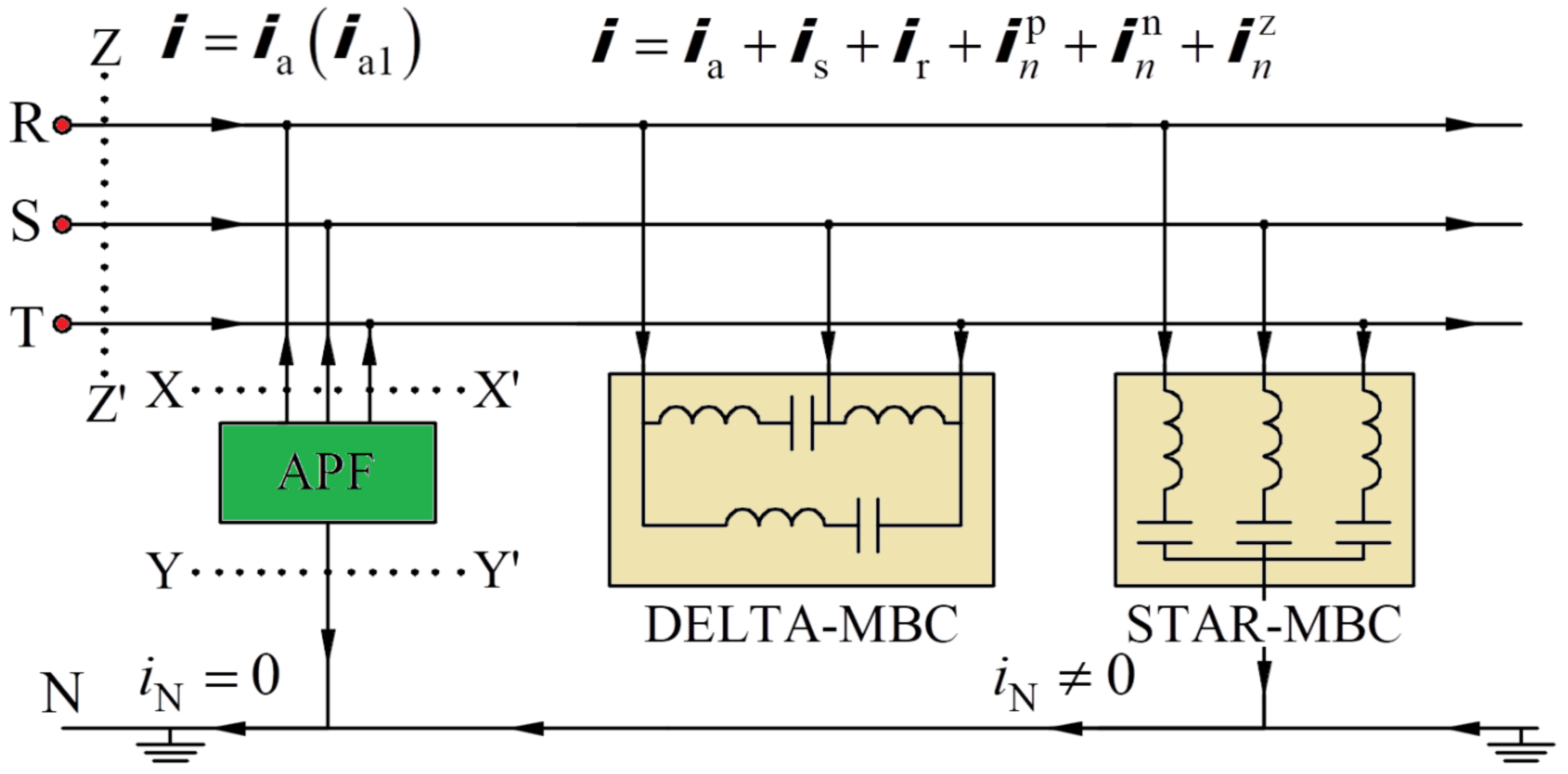
Figure 7 shows an example of APF connection to the LTI load.

As has already been mentioned in Chapter 5, due to the use of the minimizing balancing compensation, the power factor (22) was equal to 0.986. Using the system of Equations (43) and (44), we can obtain the power factor equal to 1.

It should be noted, however, that the definition of this power factor consists of the sum of the active powers P and the sum of apparent powers S. If we define the power factor as the value of the active power of the fundamental harmonic $P_1$ or the value of the active current of the fundamental harmonic ${\mathit{i}}_{\mathrm{a}1}$, then the power factor ${\lambda }_{\hspace{0.17em}1}$:

$${\lambda }_{\hspace{0.17em}1}=\frac{P_1}{P}=\frac{{\mathit{i}}_{\mathrm{a}1}}{{\mathit{i}}_{\mathrm{a}}},$$

(45)

It will still be lower than unity and it will be 0.979.

To obtain the active current of the fundamental harmonic, the relation (43) should be modified to the form:

$$i_{\mathrm{RST}ref}\left(t\right)=\left\{\begin{array}{c}{i}_{\mathrm{R}ref}\left(t\right)=-\sqrt{2}\mathrm{Re}\left\{{\displaystyle \sum _{n=2}^N}{i}_{\mathrm{aR}n}\left(t\right)+{\displaystyle \sum _{n=1}^N}{i}_{\mathrm{rR}n}\left(t\right)+{\displaystyle \sum _{n=1}^N}{i}_{\mathrm{sR}n}\left(t\right)+{\displaystyle \sum _{n=1}^N}{i}_{\mathrm{uR}n}^{\mathrm{p}}\left(t\right)+{\displaystyle \sum _{n=1}^N}{i}_{\mathrm{uR}n}^{\mathrm{n}}\left(t\right)+{\displaystyle \sum _{n=1}^N}{i}_{\mathrm{uR}n}^{\mathrm{z}}\left(t\right)\right\}\hfill \\ i_{\mathrm{S}ref}\left(t\right)=-\sqrt{2}\mathrm{Re}\left\{{\displaystyle \sum _{n=2}^N}{i}_{\mathrm{aS}n}\left(t\right)+{\displaystyle \sum _{n=1}^N}{i}_{\mathrm{rS}n}\left(t\right)+{\displaystyle \sum _{n=1}^N}{i}_{\mathrm{sS}n}\left(t\right)+{\displaystyle \sum _{n=1}^N}{i}_{\mathrm{uS}n}^{\mathrm{p}}\left(t\right)+{\displaystyle \sum _{n=1}^N}{i}_{\mathrm{uS}n}^{\mathrm{n}}\left(t\right)+{\displaystyle \sum _{n=1}^N}{i}_{\mathrm{uS}n}^{\mathrm{z}}\left(t\right)\right\} \hfill \\ i_{\mathrm{T}ref}\left(t\right)=-\sqrt{2}\mathrm{Re}\left\{{\displaystyle \sum _{n=2}^N}{i}_{\mathrm{aT}n}\left(t\right)+{\displaystyle \sum _{n=1}^N}{i}_{\mathrm{rT}n}\left(t\right)+{\displaystyle \sum _{n=1}^N}{i}_{\mathrm{sT}n}\left(t\right)+{\displaystyle \sum _{n=1}^N}{i}_{\mathrm{uT}n}^{\mathrm{p}}\left(t\right)+{\displaystyle \sum _{n=1}^N}{i}_{\mathrm{uT}n}^{\mathrm{n}}\left(t\right)+{\displaystyle \sum _{n=1}^N}{i}_{\mathrm{uT}n}^{\mathrm{z}}\left(t\right)\right\} \hfill \end{array}\right.$$

(46)

Compensation of the current in the neutral wire will still be achieved with the use of the reference current described by Equation (44), because the zero sequence active current is associated with each harmonic, including the fundamental harmonic.

By using Equations (44) and (46), it is possible to receive the power factor $\lambda$ equal to unity and associated with the fundamental harmonic of the active current. The waveform of the active current of the fundamental harmonic will have the same asymmetry as the fundamental harmonic of the voltage waveform.

7. Theoretical and Simulation Illustration—The Analysis of the System with an Active Power Filter Connected

The summary of the theoretical analysis is the determination of the reference currents in the X-X’ and Y-Y’ cross-sections and the depiction of the waveforms of the line current that can be obtained on the basis of the relationship (43) and (46) in the Z-Z’ cross-section.

Figure 8 does not present the load considered earlier, only the minimizing balancing compensators (DELTA-MBC and STAR-MBC) and the connected energy power filter (APF) with marked cross-sections that will be considered.

Basing the APF control algorithm based on the relationship (43), the waveform of the three-phase reference current is received, shown in Figure 9.

Based on the reference current generated in this way (Figure 9) and the relationship (43) in the cross-section Z-Z’, a nonsinusoidal active current waveform will be obtained as shown in Figure 10.

Due to the use of the passive compensation in the form of the minimizing balancing compensation, it was capable to reduce the RMS value of the currents in the respective lines (

Table 7. List of the RMS value of the currents of the lines before compensation and after using the passive and active compensation.

Phase	RMS Value [A]
	BEFORE	MBC	APF (43)	APF (46)
R	162.97	105.93	104.95	102.25
S	106.10	99.37	98.34	95.58
T	220.62	101.19	100.67	97.80
$‖\mathit{i}‖$	294.09	177.02	174.46	170.75
N	180.75	62.96	0	0

). The application of the active filtration and the injection of the reference currents to the supply lines will contribute to a further reduction in the RMS value of the currents of the line.

The values presented in Table 7 have been calculated based on an algorithm written in the form of a script in the Matlab software. The algorithm created in Matlab was based on the relationships described in Section 2, Section 4, and Section 6.

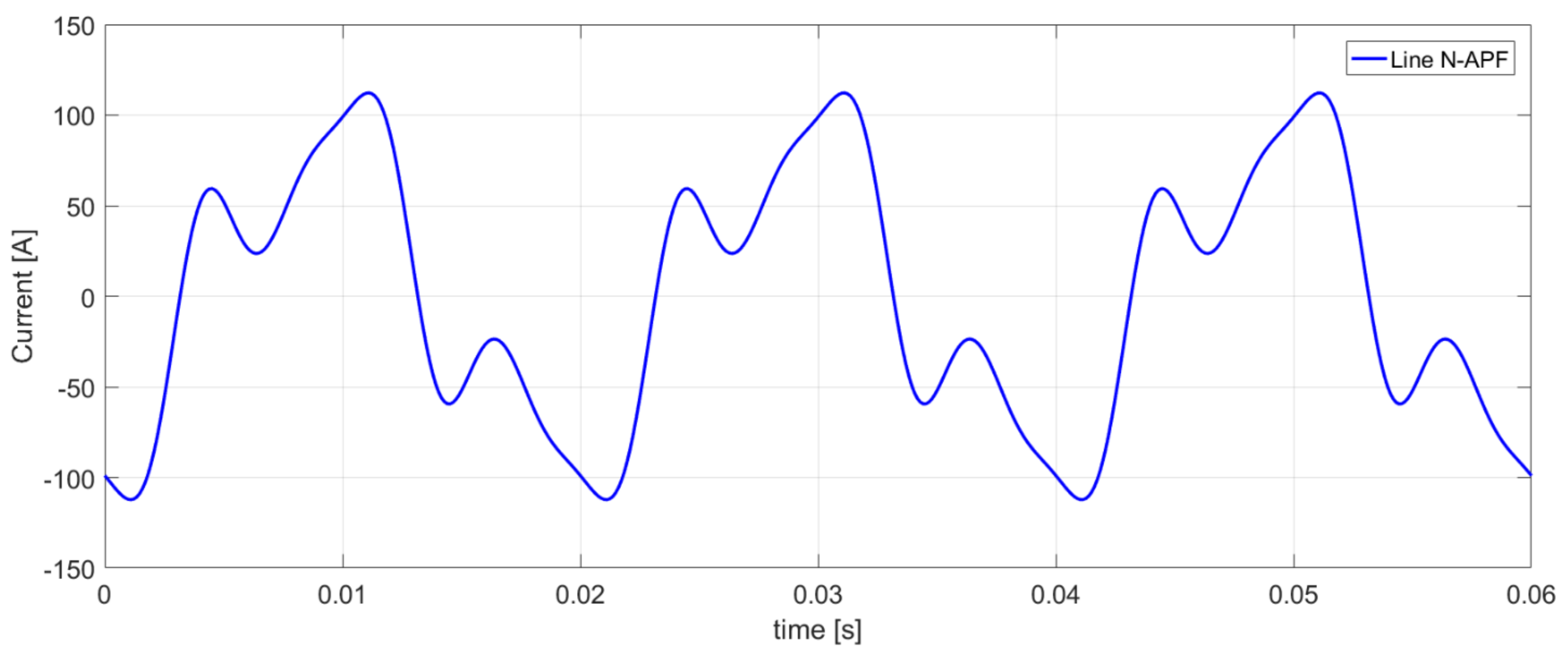
Based on Equation (44), the reference current injected into the neutral wire (cross-section Y-Y’) has the waveform shown in Figure 11.

Due to the use of passive compensation in the form of the minimizing balancing compensation, it was possible to reduce the RMS value of the current in the neutral wire (Table 7). The use of active filtration and the injection of the reference current (44) to the neutral wire will contribute to the complete (in a theoretical example) compensation of the current (Table 7).

Based on the APF control algorithm ensuing from Equation (46), the waveform of the three-phase reference current is obtained, as shown in Figure 12.

Based on the reference current generated in this way (Figure 12) and the relation (46) in the Z-Z’ cross-section, a sinusoidal active current waveform is obtained (Figure 13).

The application of the active filtration expressed in relation (46) and the injection of the reference currents to the supply lines will contribute to a further reduction of the RMS values of the currents of the lines (Table 7).

As can be seen from Figure 13, the waveform of the active currents in the respective lines is charged with the difference in amplitude and phase shift, as it responds to the values of amplitude and phase shift in the supply voltage of the fundamental harmonic. When using CPC theory (approach for the description of systems with asymmetrical voltage waveforms) as a method for generating reference currents, it should be remembered that without symmetrization of the voltage supply, the active currents (version with sinusoidal or nonsinusoidal waveforms), will reflect the amplitude and phase asymmetry present in this supply voltage.

8. Conclusions

The article presents an unbalanced linear time-invariant load supplied with asymmetrical nonsinusoidal voltage in four-wire systems. It can be almost perfectly balanced and its reactive power can be compensated also almost perfectly. The use of the minimizing balancing compensation (the passive part of the hybrid filter) increases the power factor to a value close to unity. The application of an active power filter results in additional benefits of the compensation of the reactive, scattered, and unbalanced currents that cannot be compensated using passive elements in the form of the minimizing balancing compensator.

The solution proposed on the basis of Equation (43) in generating reference currents results in obtaining only the nonsinusoidal active current. In such an approach, the reactive power and the unbalanced power do not exist, because the active current waveform is identical to the nonsinusoidal supply voltage waveform (there is no shift between voltage and current waveform). The second approach, which is described with the relation (46), focuses only on obtaining a sinusoidal active current reflecting the voltage waveform of the fundamental harmonic. Additionally, the second approach improves the stability and energy efficiency of the supply network.

The control methods of APF proposed in the article clearly show the possibility of including the asymmetry of the supply voltage, which is so often omitted by other authors. The phenomenon of voltage asymmetry is present to a greater or lower rank in every supply system. As it has been shown in the article, accepting this phenomenon allows the correct mathematical description of LTI loads and, at the same time, contributes to a more precise control of generation of the reference current of the APF. This is because previously no one considers the three coefficients of asymmetry, which together can correctly describe the admittance dependent on voltage asymmetry.

The authors of the article, for some time, have been focusing on the correct description of energy properties, which are closely related to physical phenomena. Due to this approach, a correct mathematical description is obtained, which is a further stage to use for theoretical and then real improvement of the power supply conditions in single- or three-phase systems.