Electric Vehicle Charger Static and Dynamic Modelling for Power System Studies

Abstract

Electric Vehicles (EVs) are becoming increasingly available and are expected to be a large part of the load in future power systems. EV chargers are a relatively new type of load and are mainly interfaced with the grid through power electronics. It is therefore important to investigate the impact they have on power system dynamic behaviour. In this paper, two detailed EV charger models (representing a typical slow and fast charger) were investigated. The aim was to test the capability of standard static—and more importantly, dynamic—load models, commonly used in power system studies, to represent the static and dynamic behaviour of EV chargers. Different control parameter settings for two types of EV chargers were investigated, as were the limits of standard power system dynamic load model structures’ accurate representation. Typical parameter sets have also been provided for cases where proper representation was possible.

1. Introduction

In several countries, electric vehicles (EVs) are being introduced at a fast pace. This change is driven to a large extent by efforts to decarbonise transport, but technical and economic advancements are also factors. In 2018, the global electric car fleet exceeded 5.1 million—an increase of 2 million compared to the previous year [1]. Due to the fast pace of integration of EVs, EV chargers might become a significant part of the electric load, especially in certain locations and in certain times of the day. This would, of course, depend on the potential charging behaviour of users. EV chargers are mainly interfaced with the grid through power electronic converters which might exhibit different dynamic behaviour compared to traditional loads. The static and (most importantly) dynamic behaviour of EVs is expected to play an important role in stability analysis of power systems. Therefore, representative models (capturing both static and dynamic parts) need to be developed, established and investigated in order to conduct credible power system stability simulations. Moreover, there is a need to determine whether traditional power system dynamic load models are capable of representing EV charger dynamic behaviour—a question this paper begins to address.

A large amount of research has been conducted which focused on static studies and the economics of EVs [2], with emphasis on the electricity peak demand and system stress of EV charging [3,4,5,6]. It is also important to investigate the static and dynamic behaviour of EVs beyond charging profiles and geographical distribution—and into system stability aspects [6,7,8]. Additionally, an effort to investigate the static load behaviour of EV chargers is available in the literature. Typical parameters to fit both the standard ZIP (Z for impedance, I for current and P for power) and exponential static load models (commonly used in power system studies) have been proposed [5,9,10]. With respect to dynamic responses of EVs, detailed modelling approaches were introduced in [11,12,13], representing in detail the power electronic interfaces of EV chargers. Such approaches can represent in detail the dynamic behaviour of EV chargers, including G2V (grid-to-vehicle), V2G (vehicle-to-grid) and residential charging [14,15,16,17,18]. However, such models are not practical for use in large-scale power system stability and dynamic studies due to the complexity and increased computational effort required.

It should also be noted that there are several charging standards and power levels available for EV chargers, ranging from slow to fast and super-fast. The Electric Power Research Institute (EPRI) and Society of Automotive Engineers (SAE) have categorized EV charging level as AC level-1, AC level-2 and DC fast charging, i.e., level-3 [4,19]. Some examples include the AC level-2 at 7.4 kW, DC fast charging level-3 at 50 kW, and super-fast chargers like Tesla superchargers at 350 kW or CHAdeMO 2.0 at 400 kW. It should be noted that wireless charging is also emerging; however, the investigation of wireless chargers falls out of the scope of this paper since it has not yet been widely adopted [20]. In this paper, two different typical charging approaches were chosen: a 7.4 kW level-2 charger (commonly used in residential applications and suitable for a 230V power supply [21]) and a 50 kW DC fast charger (i.e., level-3 DC charge [22]). Detailed dynamic models—including the switching behaviour of power electronic converters—were implemented and used to test the capability of typical static load models (ZIP and exponential [5,9,10]) for both charging approaches.

This paper focused on the load modelling of EV charging in power systems, with the ultimate purpose of studying and investigating the impact of EVs on power system stability. It investigated the extent to which standard static and dynamic load models used in power system studies could represent typical slow and fast EV chargers, as well as their sensitivity to changes in control parameters. Complex detailed models (including the detailed behaviour of power electronics) were initially used to extract parameters for typical load models used in power system studies, following a curve fitting approach. In more detail, the key contributions of the paper were the following: (i) detailed models were used to test the capability of a standard dynamic load model commonly used in power system dynamic studies—namely, the exponential recovery dynamic load model [23,24,25,26]—to represent EV charger dynamic behaviour. Curve fitting was used to define appropriate model parameters for both the static and dynamic load models. (ii) Different control settings (i.e., PI—Proportional and Integral gains) for both charging approaches were investigated, showcasing the impact they have on the ability of the exponential recovery dynamic load model to accurately represent the response of EV chargers. (iii) A comparison of both static and dynamic load model characteristics for different EV charging approaches (i.e., a typical slow and fast charger). Ultimately, the paper presents sets of parameters that can be utilised to represent EV charger behaviour for certain control settings and for both static and dynamic responses. Thus, the paper offers insight on potential limitations of standard models in representing EV charger dynamic behaviour.

2. Load Modelling and Curve Fitting

Load models can be generally divided into static and dynamic, effectively characterising the responses of active and reactive power to certain power system conditions. The static load model expresses load characteristics by algebraic functions at any instant of time. Since it does not contain any dynamic information, the dynamic load model is necessary to analyse power system dynamic behaviour in small and large disturbances. In this section, both static and dynamic load models for EV charging approaches are analysed in detail.

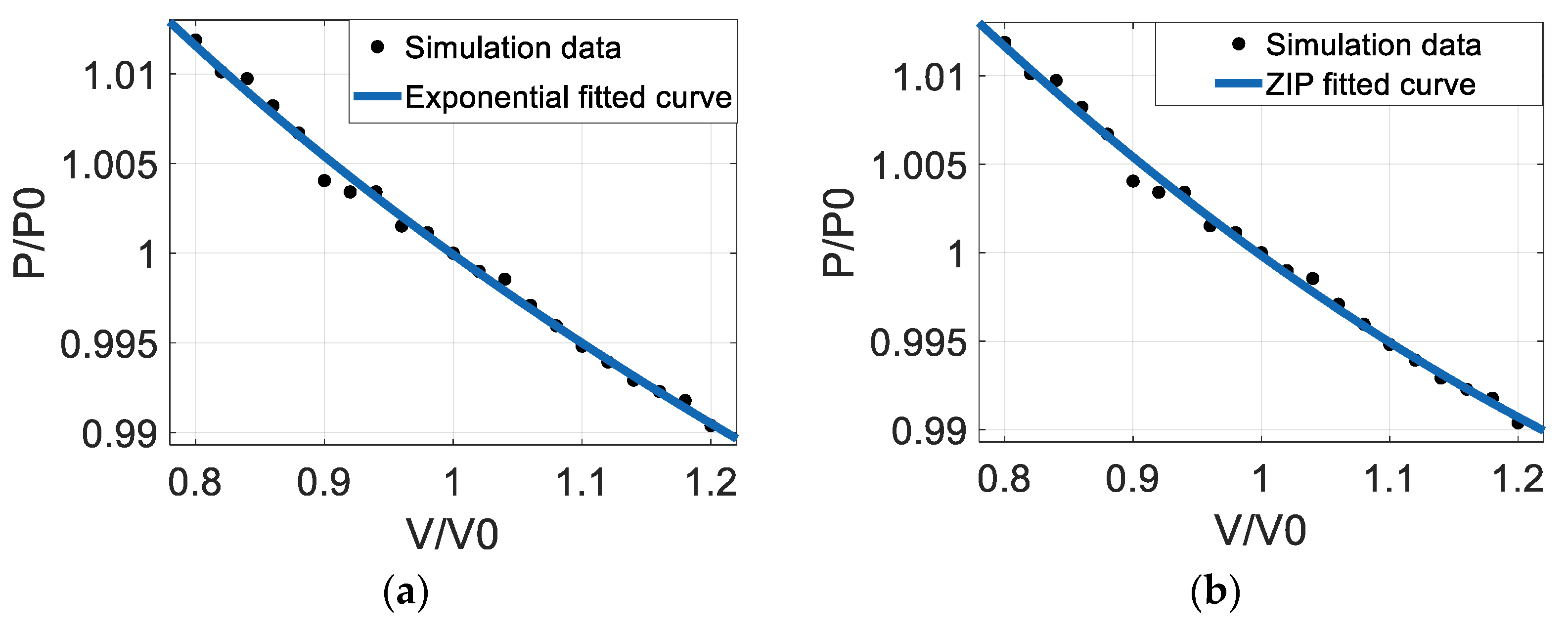
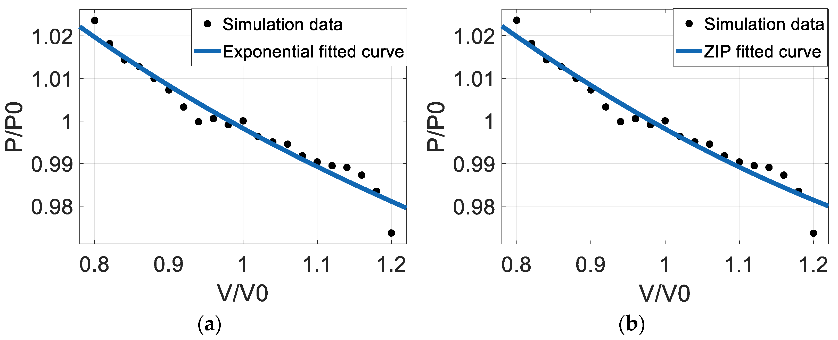
2.1. Static Load Models

Static load models are generally used to calculate the steady-state behaviour of loads. Since the static load model does not consider any dynamic behaviour, power system loads (including EVs) can be modelled as static ones, capturing their sensitivity in terms of both active and reactive power. Two typical, commonly used static load models were used in this paper: a polynomial load model (ZIP model) and an exponential load model. Both models represent the relationship between the voltage supply and power consumption but have different mathematic functions— i.e., polynomial function and exponential function. The expressions of active and reactive power described within the ZIP are presented in Equations (1) and (2), respectively [23].

$${\mathrm{P} = \mathrm{P}}_0[{\mathrm{p}}_1{\overline{\mathrm{V}}}^2+{\mathrm{p}}_2\overline{\mathrm{V}}+{\mathrm{p}}_3]$$

(1)

$$\mathrm{Q}={\mathrm{Q}}_0[{\mathrm{q}}_1{\overline{\mathrm{V}}}^2+{\mathrm{q}}_2\overline{\mathrm{V}}+{\mathrm{q}}_3]$$

(2)

${\mathrm{V}}_0$${\mathrm{P}}_0$${\mathrm{Q}}_0$ represent the voltage, active power, and reactive power when the supply voltage corresponds to 1 p.u. In Equations (1) and (2), ${\mathrm{p}}_1-{\mathrm{p}}_3$ and ${\mathrm{q}}_1-{\mathrm{q}}_3$ are the model parameters which—when they approach 1—imply that the load behaves as a constant impedance, constant current or constant power, respectively. The independent parameter $\overline{\mathrm{V}}$ from (3) is the per-unit supply voltage. If the actual voltage supply is equal to the nominal voltage ${\mathrm{V}}_0$, then $\overline{\mathrm{V}}$ will be also equal to 1, as shown in (3).

$$\overline{\mathrm{V}}=\frac{\mathrm{V}}{{\mathrm{V}}_0}$$

(3)

The exponential model [23,27,28] has essentially two parameters to describe the relationship of active and reactive power with respect to voltage: α and β, as shown in Equations (4) and (5) below:

$$\mathrm{P}={\mathrm{P}}_0{(\overline{\mathrm{V}})}^{\mathrm{\alpha }}$$

(4)

$$\mathrm{Q}={\mathrm{Q}}_0{(\overline{\mathrm{V}})}^{\mathrm{\beta }}$$

(5)

As opposed to the ZIP model, there is only one parameter to describe active power and reactive power exchange with respect to the voltage supply. When parameter α and β are close to 2, this implies that the load can be seen as a constant impedance. When parameters α and β approach 1 it means that the load can be seen as constant current. Finally, when parameters α and β are close to 0, the active and reactive power exchange does not change with respect to voltage. This means that the load behaves as constant power.

As previously explained, the detailed EV charger models for approaches A and B (where A is a relatively slower typical AC/DC charger, and B is a typical DC fast charger, both of which are explained in detail in Section 3) were used to obtain static values and consequently characterise the static behaviour of typical EV chargers using the two standard load model structures. For this reason, curve fitting was used to approximate the load parameters of the target expressions (i.e., Equations (1), (2), (4) and (5)) using simulation-based data. After conducting a wide range of simulations and extracting the results (i.e., voltage and active power), an exercise to approximate the load parameters (i.e., ${\mathrm{p}}_1$ ${\mathrm{p}}_2$ and ${\mathrm{p}}_3$ in ZIP model) was put forward. The chosen methodology to obtain the parameters was the least-squares method [23]. Such a method requires the target equation as well as the response data (i.e., results extracted from simulations). Effectively, the least-squares method minimises the sum s of the squared offsets or residuals of points from a curve:

$$\mathrm{s} = {\displaystyle \sum }_{\mathrm{i}=1}^{\mathrm{n}}{({\mathrm{y}}_{\mathrm{i}}-\widehat{{\mathrm{y}}_{\mathrm{i}}})}^2$$

(6)

where s is the sum of squares error estimate, ${\mathrm{y}}_{\mathrm{i}}$ the observed response and $\widehat{{\mathrm{y}}_{\mathrm{i}}}$ the fitted response value. The curve fitting result chooses the parameter which provides the lowest error estimate s. For the studies presented in this paper, ‘cftool’ from Matlab Math, Statistics and Optimization library was utilised.

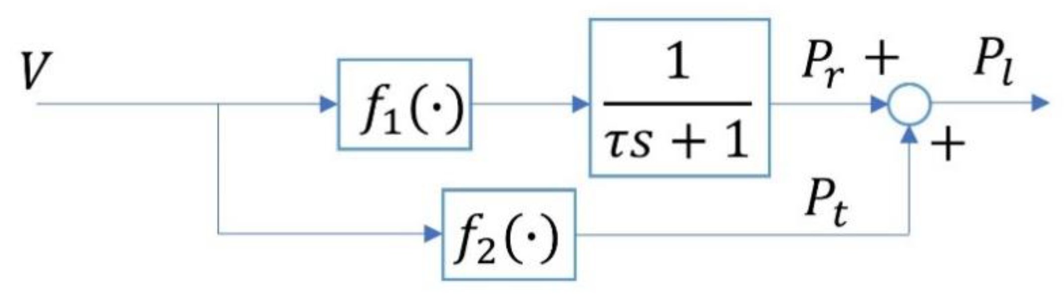
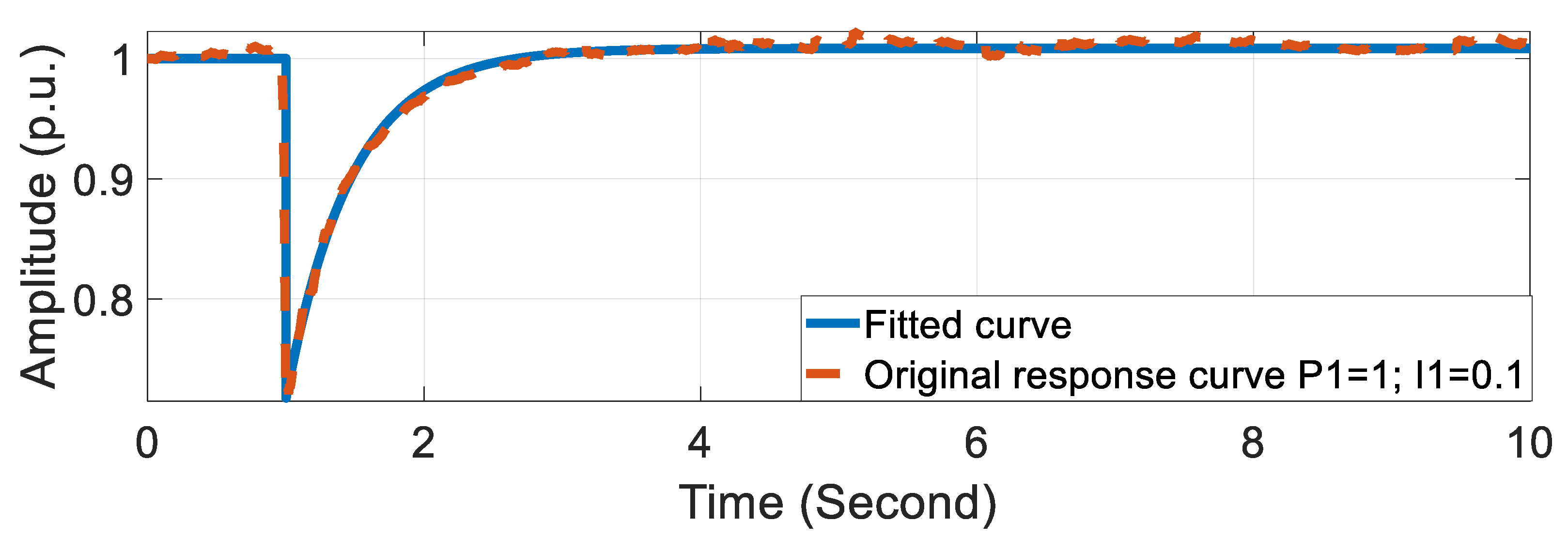
2.2. Dynamic Load Models

The dynamic load model is an extension of the static load models used to capture and represent faster phenomena-like disturbances. It should be noted that the dynamic load model used in this paper is also called the exponential recovery model in the literature. It is different from the exponential static load model presented in the previous section. From the research conducted in [24,25], the parameters ${\left(\frac{\mathrm{V}}{{\mathrm{V}}_0}\right)}^{{\mathrm{a}}_{\mathrm{s}}}$ and ${\left(\frac{\mathrm{V}}{{\mathrm{V}}_0}\right)}^{{\mathrm{a}}_{\mathrm{t}}}$(which come from static load model exponential parameters) can represent the steady-state values before and after a disturbance. Based on [24,25], one of the standard dynamic load models used in power system dynamic studies is the exponential recovery load model, represented by (7) and (8).

$${\mathrm{T}}_{\mathrm{p}}\frac{{\mathrm{dP}}_{\mathrm{r}}}{\mathrm{dt}}+{\mathrm{P}}_{\mathrm{r}}={\mathrm{P}}_{\mathrm{s}}\left(\mathrm{V}\right)-{\mathrm{P}}_{\mathrm{t}}\left(\mathrm{V}\right)={\mathrm{P}}_0(\frac{\mathrm{V}}{{\mathrm{V}}_0}{)}^{{\mathrm{a}}_{\mathrm{s}}}-{\mathrm{P}}_0(\frac{\mathrm{V}}{{\mathrm{V}}_0}{)}^{{\mathrm{a}}_{\mathrm{t}}}$$

(7)

$${\mathrm{P}}_{\mathrm{l}}={\mathrm{P}}_{\mathrm{r}}+{\mathrm{P}}_0(\frac{\mathrm{V}}{{\mathrm{V}}_0}{)}^{{\mathrm{a}}_{\mathrm{t}}}$$

(8)

P_l from (8) is the overall power consumption and $P_r$ the power recovery part (explained in more detailed below). From [23], the overall response of the dynamic load model can be represented by (9). The expression in (9) is characterised by a static part (i.e., ${\mathrm{P}}_0{\left(\frac{\mathrm{V}}{{\mathrm{V}}_0}\right)}^{{\mathrm{a}}_{\mathrm{t}}}$ and ${\mathrm{P}}_0{\left(\frac{\mathrm{V}}{{\mathrm{V}}_0}\right)}^{{\mathrm{a}}_{\mathrm{s}}}$) and a dynamic part $\left(1-{\mathrm{e}}^{\raisebox{1ex}{$-\mathrm{t}$}\!\left/ \!\raisebox{-1ex}{${\mathrm{T}}_{\mathrm{p}}$}\right.}\right)$, which is essentially a first-order system.

$${\mathrm{P}}_1(\mathrm{t})=\left[\left({\mathrm{P}}_0{\left(\frac{\mathrm{V}}{{\mathrm{V}}_0}\right)}^{{\mathrm{a}}_{\mathrm{s}}}-{\mathrm{P}}_0{\left(\frac{\mathrm{V}}{{\mathrm{V}}_0}\right)}^{{\mathrm{a}}_{\mathrm{t}}}\right)\left(1-{\mathrm{e}}^{-\mathrm{t}/{\mathrm{T}}_{\mathrm{p}}}\right)+{\mathrm{P}}_0{\left(\frac{\mathrm{V}}{{\mathrm{V}}_0}\right)}^{{\mathrm{a}}_{\mathrm{t}}}\right]\alpha$$

(9)

It should be noted here that the static part ${\mathrm{P}}_0{\left(\frac{\mathrm{V}}{{\mathrm{V}}_0}\right)}^{{\mathrm{a}}_{\mathrm{s}}}$ was taken from the results obtained in the previous section. A range of dynamic simulations were performed using detailed EV charging models. Based on them, the parameters ${\mathrm{P}}_{\mathrm{r}}$ and ${\mathrm{T}}_{\mathrm{p}}$ (corresponding to the dynamic part of the expressions in (9)) were obtained by utilising the curve fitting tool. The adopted dynamic load model includes both a static and dynamic part—which can be used to represent the dynamic response through equation (9).

In this paper, the well-established exponential recovery load model (ERLM) was utilised to realise the curve fitting of the EVs dynamic responses [24,25,29]. This model decomposed the dynamic power consumption of the load ${\mathrm{P}}_{\mathrm{l}}$ into two main parts: ${\mathrm{P}}_{\mathrm{r}}$ and ${\mathrm{P}}_{\mathrm{t}}$. ${\mathrm{P}}_{\mathrm{r}}$ represents the power recovery and P_t represent s the transient nonlinear characteristic of the load. Consequently, ${\mathrm{f}}_1\left(·\right)$ would correspond to the term $({\mathrm{P}}_0{\left(\frac{\mathrm{V}}{{\mathrm{V}}_0}\right)}^{{\mathrm{a}}_{\mathrm{t}}}{-\mathrm{P}}_0{\left(\frac{\mathrm{V}}{{\mathrm{V}}_0}\right)}^{{\mathrm{a}}_{\mathrm{s}}}$) from (9) and ${\mathrm{f}}_2\left(·\right)$ to the term ${\mathrm{P}}_0{\left(\frac{\mathrm{V}}{{\mathrm{V}}_0}\right)}^{{\mathrm{a}}_{\mathrm{t}}}$. In this paper, the dynamic part of the equation (9) was used with the curve fitting tool to obtain parameters that matched the detailed simulation results from the EV charger models following approaches A and B, as presented in Section 3. The parameters applicable to equation (9) can be obtained through the diagram shown in Figure 1, which has been adopted by [23,29].

A curve fitting methodology for power system dynamic response was provided in [25]. This method decomposed the dynamic response of the model into two main parts. In this paper, the dynamic part of Equation (9) was used with the curve fitting tool to obtain parameters that matched the detailed simulation results from the EV charger models following approaches A and B. Figure 1 provides an example of the curve fitting. The exponential recovery load model accurately represented the EV charger by following approach A for the given set of PI parameters (sensitivity to which will be investigated later in this paper).

Figure 2 presents an example of the curve fitting approach for a particular case in which the EV charger response fit well with the dynamic load model response presented in (9). To quantify the effectiveness of curve fitting, this paper used two coefficients, the R-squared and normalized root-mean-square error (NRMSE). R-squared was shown in (10) and used to evaluate the fitting results by utilising measurement data $\mathrm{y}$, the estimated response $\widehat{\mathrm{y}}$ and the mean value $\overline{\mathrm{y}}$:

$$\mathrm{R}-\mathrm{squared} = 1 - \frac{\sum {\left(\mathrm{y}-\widehat{\mathrm{y}}\right)}^2}{\sum {\left(\mathrm{y} -\overline{\mathrm{y}}\right)}^2}$$

(10)

The R-squared is a common parameter in statistics used to show the degree of similarity between the fitting result and the target. When the R-squared is close to 1, it implies that the fitted curve is very similar to the original data. Effectively, if R-squared approaches 1, the dynamic load model used in this paper can adequately describe the dynamic features of EVs while considering different levels of voltage disturbances.

NRMSE is based on the root-mean-square error (RMSE), which is frequently used to measure the differences between predicted and observed values, as shown in (11). The NRMSE facilitates comparison between datasets with different scales. In this study, scale parameters were determined by the amplitude of dynamic responses with maximum value ${\mathrm{y}}_{\max }$ and minimum value ${\mathrm{y}}_{\min }$, as presented in (12).

$$\mathrm{RMSE}=\sqrt{\frac{{{\displaystyle \sum }}_{\mathrm{t}=1}^{\mathrm{T}}{\left(\mathrm{y}-\hat{\mathrm{y}}\right)}^2}{\mathrm{T}}}$$

(11)

$$\mathrm{NRMSE}=\frac{\mathrm{RMSE}}{{\mathrm{y}}_{\max }-{\mathrm{y}}_{\min }}$$

(12)

Contrary to the R-squared value, a smaller NRMSE value indicates a higher fitting quality. Comparing these two methods, R-squared provided results between 0 and 1, while NRMSE was not constrained to any particular values. Although R-squared (taking values between 0 and 1) might be more descriptive, both metrics were used and reported in this paper for completeness.

3. Detailed EV Charger Models

In this Section, two typical models were adopted and used to represent a slow (7.4 kW level-2 charger) and fast charger (50 kW DC fast charger). These were implemented in detail in Matlab/Simulink (CPU: Intel i7-8750H; Software: Matlab/Simulink 2019a) in order to obtain detailed responses of standard EV chargers for small voltage disturbances. Consequently, simulated responses from these models were used to derive the data used in curve fitting approaches for both the static (using steady-state values) and dynamic (using time domain responses) load models. The slow charge approach (approach A) was based on a diode rectifier and a DC/DC converter [30,31] while the fast charge approach (approach B) utilised a three-phase full bridge converter and a DC/DC converter [10,32]. Approach A was characterised by simplified control structures, which made it popular for earlier EV charging stations—such as small residential chargers (e.g., level-2, 7.4 kW). However, approach A had functional limitations (i.e., unidirectional power flow) which rendered it inappropriate for smart charging applications. Approach B was characterised by the possibility of bidirectional power flows and fast charging features. For rapid charging, 50 kW chargers are widely (e.g., ABB Terra 53 [33] and Delta DC 50 kW quick charger [34]); thus, a 50kW charging level was chosen for approach B in this paper.

3.1. Approach A–Typical EV Slow Charger

Charging approach A consisted physically of two main parts—a diode rectifier and a DC/DC converter, as depicted in Figure 3. This approach is commonly found in slow charging and sometimes low-power designs [9,31], e.g., electric scooters.

A large number of circuit topologies and control methods have been developed for EV and plug-in hybrid electric vehicle (PHEV) battery chargers. Two-stage power conversion (i.e., AC/DC and DC/DC) provides inherent low-frequency ripple rejection and has been used in modern battery charger topology [30].

Power factor correction (PFC) control aims to keep the power factor close to 1 and can also be implemented in charger structures. This is done by appropriately controlling the boost converter between the diode rectifier and the full bridge DC/DC converter [9,31].

Based on the structure depicted in Figure 3, several technologies can be used for each part; for example, a diode bridge can be used on the AC/DC part [11,13,35,36] due to its simplified structure. To construct a single-phase residential charging station (e.g., 7.4 kW), PFC controllers could be realised based on control loop strategies as defined in [30,31,37]. The DC/DC part could be realised by utilising full bridge DC/DC converters with current feedback control [31,35], with a series loaded resonant DC/DC converter [31], or even with a buck converter [10].

The EV charging model deployed in this paper to represent a typical slow charger (approach A) was based on the architecture described in [37], which utilised a diode rectifier, a boost converter (including PFC) and a full bridge DC/DC converter.

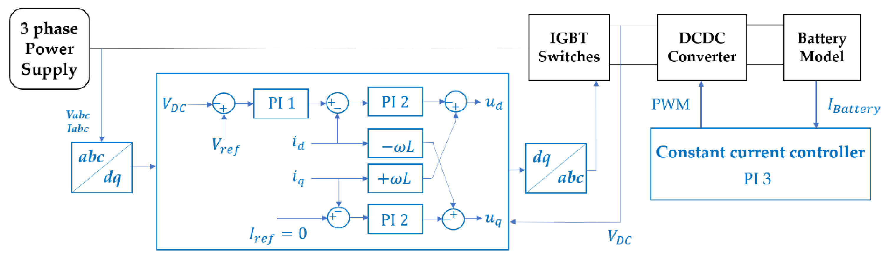
3.2. Approach B–Typical EV Fast Charger

The topology which underpins approach B physically consists of a full bridge three-phase inverter and a DC/DC converter (as shown in Figure 4 below), representing a typical EV fast charger [10].

Differing from the structure of charging approach A, the control system for approach B required a full bridge converter (i.e., a fully controllable AC/DC converter). This consisted of both outer voltage and inner current control loops [10,32]. Effectively, the inner current control loop drove the converter based on dq currents (as generated by the associated references of the outer control loops).

With a few exceptions (e.g., Tesla superchargers), there are usually DC/DC converters in EV chargers that regulate the charging DC voltage in conjunction with power flow control. Such voltage regulation can be obtained by a constant PWM (Pulse-Width Modulation) or by adding a feedback control [10].

Note that DC/DC converters were added to the models for approaches A and B to manage voltage and current control for battery charging. This is not expected to have a significant impact on the dynamic load modelling aspects discussed in this paper (an example reinforcing this is provided in Section 4.3, Figure 8). However, the models used in this paper retained these structures, as detailed model development was out of the scope of this work. Hence, state of the art models from the literature were implemented.

4. Result of EV Load Model Parameters

4.1. Static Load Model Parameters for Charging Approaches A & B

Static load modelling expressions—together with the curve fitting tool—were used to characterise the relationship between the supply voltage and active power exchange for EV chargers. The active power output at each voltage level was obtained from detailed simulations after they reached steady-state values. The curve fitting exercise was conducted for the static load model parameters for the active power, as expressed in Equation (1) and (4). The results of the fittings for the exponential and ZIP models are presented in Figure 5.

Active power did not show a significant change in the range of voltages investigated (0.8 p.u. to 1.2 p.u.), indicating that the EV charger exhibited behaviour close to a constant active power load. This was observed for the exponential and ZIP models.

In particular, the curve fitting exercise produced numerical results, as presented in

Table 1. Fitting parameter.

EV Charge Static Load Model Parameters
Charging Type	Exponential Parameter	Parameter Z	Parameter I	Parameter P
Approach A	−0.0519	0.0034	−0.1199	1.086
Approach B	−0.0921	0.0620	−0.2199	1.156

. For the exponential model, the corresponding parameter was very close to 0; for the ZIP model, the P parameter was close to 1. Such numerical results indicated that an EV could be treated as a constant power load when operating in charging approach A.

In a similar manner, the parameters for static model representation under approach B were also approximated. The simulation and curve fitting results are presented in Figure 6. The produced numerical results for the static load parameters for the exponential and ZIP models are presented in Table 1.

The overall trend of active power consumption was similar to approach A, albeit with a slightly larger deviation. Effectively, the EV charger behaviour in this case was also close to a constant power load. Table 1 confirms previous results; the active power exponential load model parameter was close to 0, while the P parameter from the ZIP model was close to 1. To summarize: the exponential and ZIP models can both represent EV charger static behaviour.

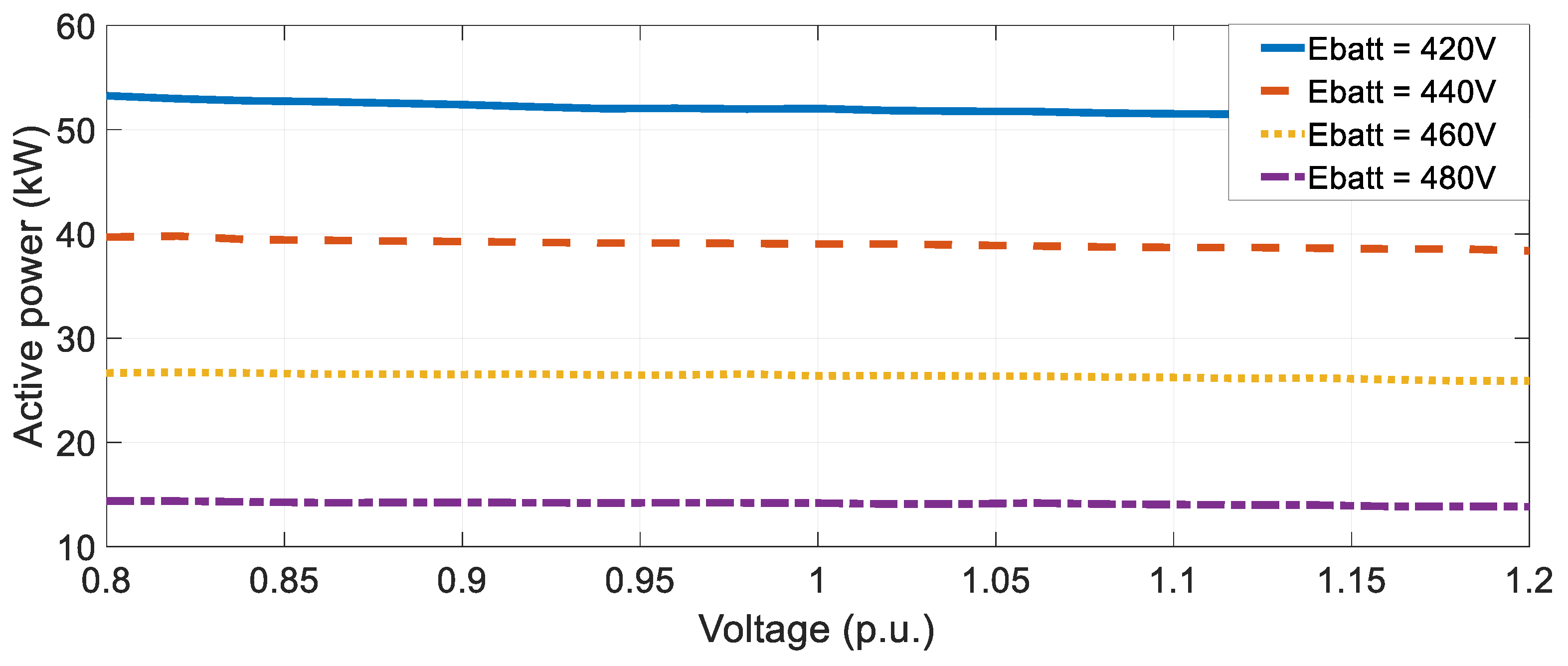
4.2. High SoC Battery Static Load Model Analysis

This work aimed to analyse the performance and subsequent load representation of EVs under different state-of-charge (SoC) conditions. This is of interest, since a DC/DC converter switches from constant current control (at low SoC levels) to constant voltage control (at high SoC levels). In both approaches, the DC/DC converters and batteries consisted of a voltage source (referred to as $E_{batt}$ in this section), a series-connected impedance, and a capacitor [10,37,38]. This structure has been utilised in other studies [5,31] and can be considered a general modelling method to represent battery voltage, impedance, and capacitance.

During a normal steady-state charging scenario, DC/DC converters provide a stable charging current into the battery by utilising constant current control. When the battery is close to fully charged, the DC/DC controller will switch to constant voltage control to reduce the charging power and prevent over-voltage and other hazardous behaviours. This section explores whether an EV can still be regarded as a constant power load in such charging circumstances. The work conducted in [17,39] revealed that battery equivalent voltage (i.e., the internal voltage source $E_{batt}$) increased significantly in a high SoC. The power flow into the battery decreased with the DC/DC converter operating in constant voltage control. As per [39,40], high SoC scenarios have been modelled by increasing the battery equivalent voltage.

A set of simulations were conducted, considering different levels of battery equivalent voltage (e.g., 420 V in normal conditions, 440 V, 460 V, and 480 V) which corresponded to higher SoCs. Charging approach B was considered for these studies. The results for active power at different voltage levels are presented in Figure 7 below. They revealed that, while the actual power level changed, the overall load static behaviour remained close to constant power (depending on the battery voltage).

By applying the curve fitting approach described previously to the results presented in Figure 7, model parameters were extracted for the exponential and ZIP models. The numerical results for different SoC levels are presented in

Table 2. Curve fitting parameters for charging approach B for different battery equivalent voltage (${\mathrm{E}}_{\mathrm{batt}}$) levels.

EV Charge Approach B
Parameter Type	Exponential Parameter	Parameter Z	Parameter I	Parameter P
${\mathrm{E}}_{\mathrm{batt}}$ = 420 V	−0.0921	0.0620	−0.2199	1.156
${\mathrm{E}}_{\mathrm{batt}}$ = 440 V	−0.0764	0.0440	−0.1651	1.12
${\mathrm{E}}_{\mathrm{batt}}$ = 460 V	−0.0683	−0.1440	0.2180	0.9283
${\mathrm{E}}_{\mathrm{batt}}$ = 480 V	−0.0821	−0.1326	0.1816	0.9495

. The parameter sets for both exponential and ZIP load models still indicated a near-constant power static behaviour from the EV charger.

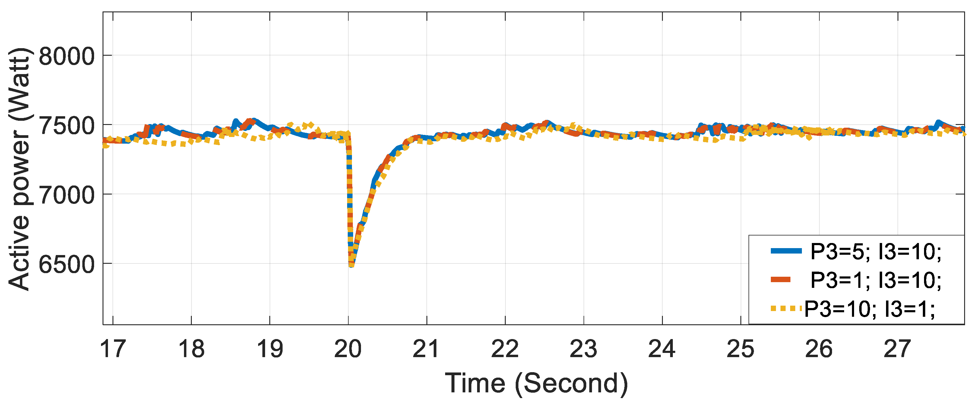
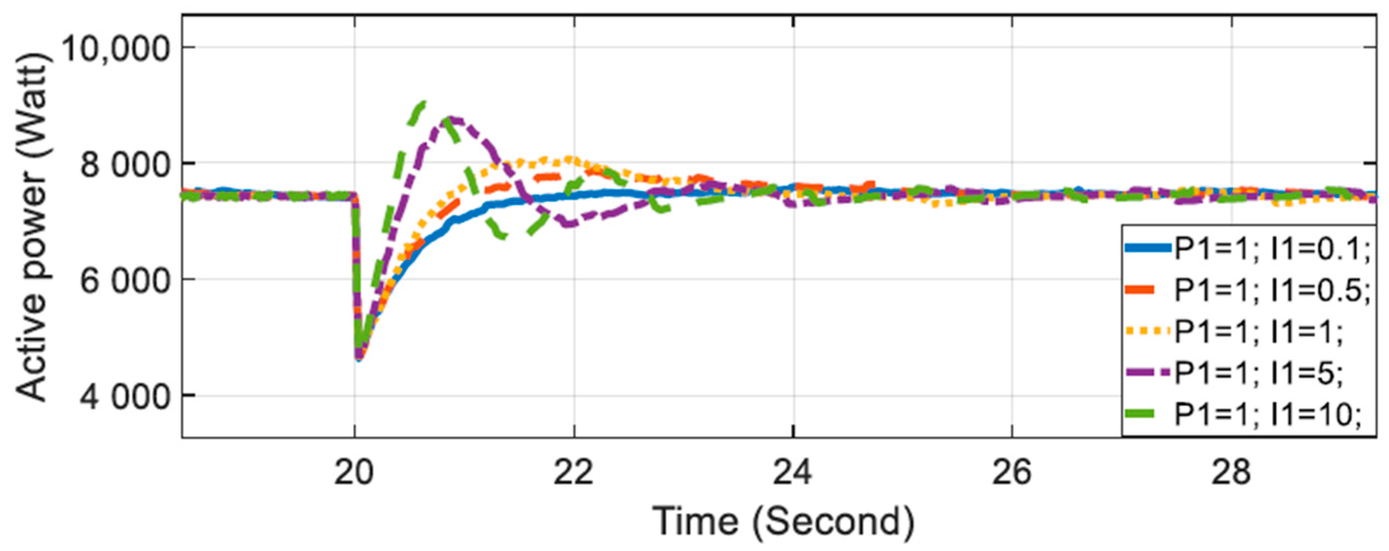
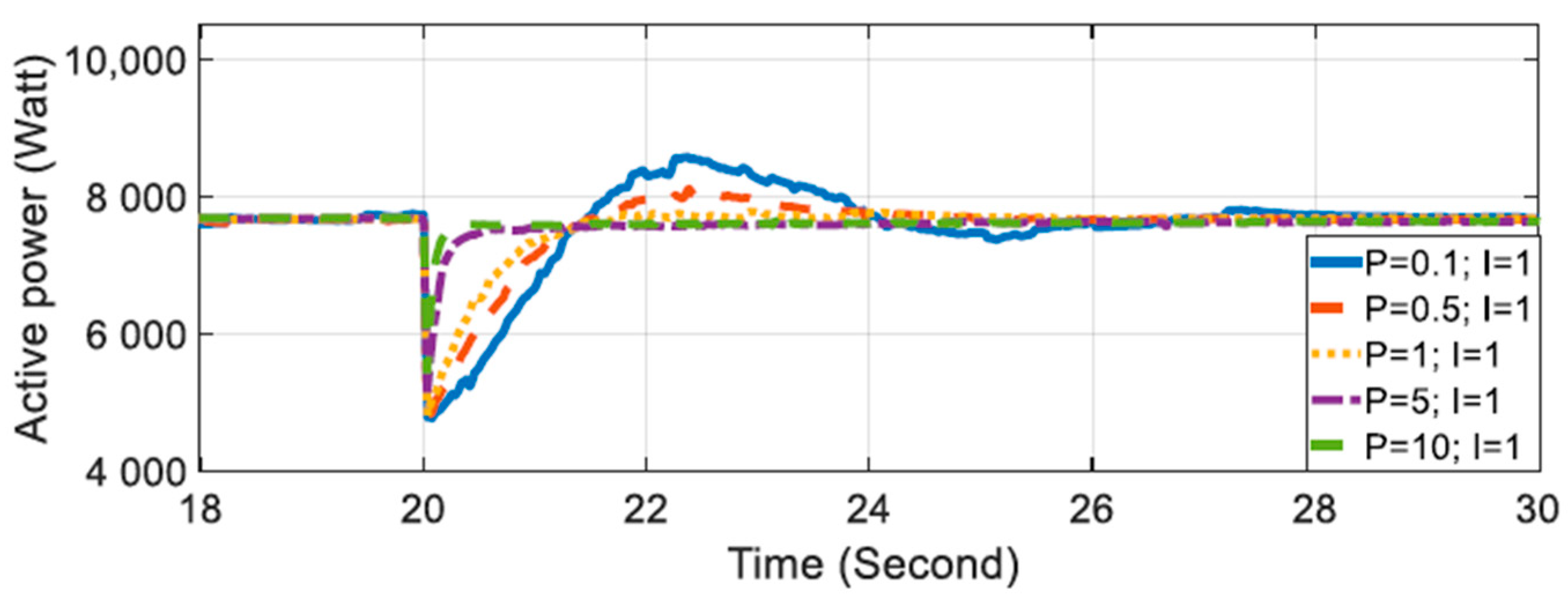
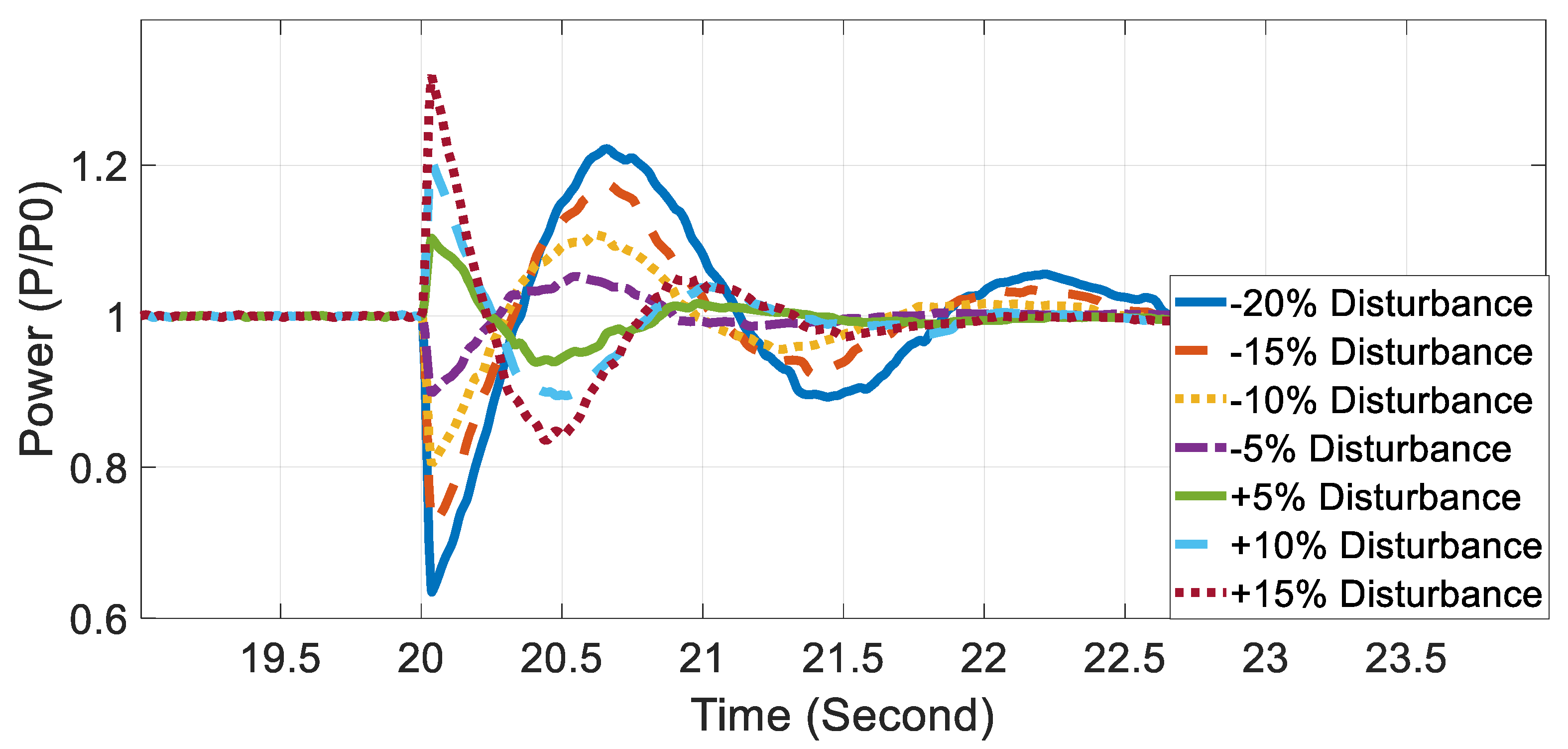
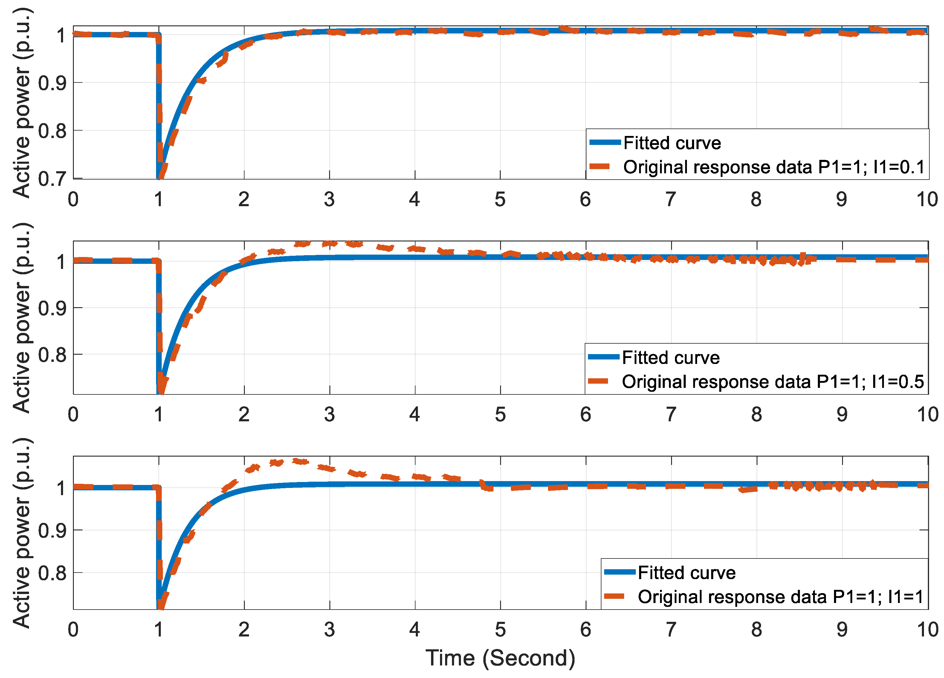
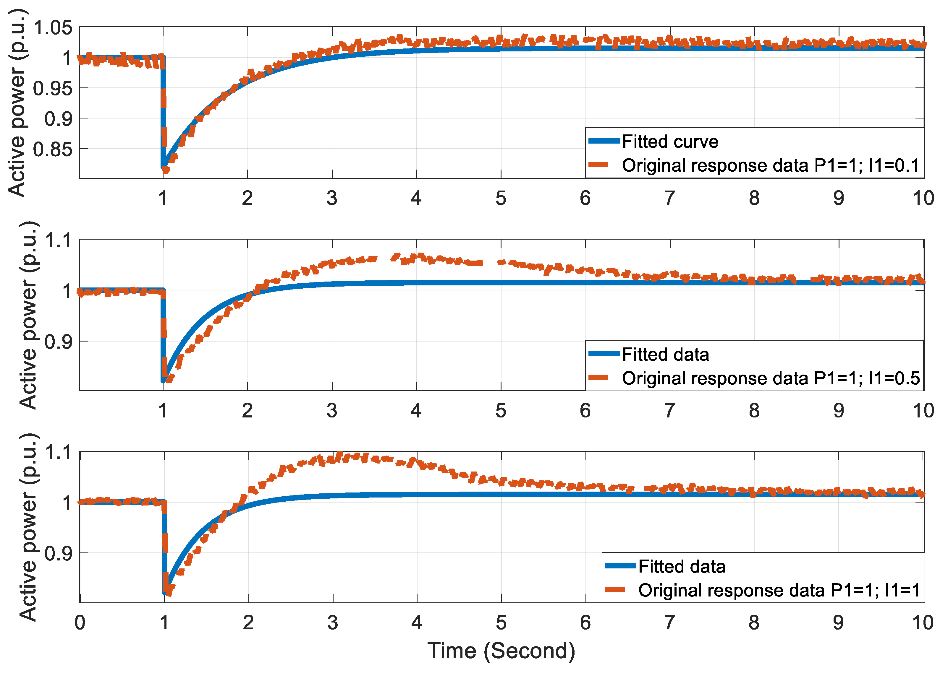
4.3. Dynamic Load Model and Control Parameter Sensitivity for Charging Approach A

The detailed EV model presented in Section 3.1 (namely charging approach A) was used to obtain dynamic responses for voltage step changes for various sets of parameters for the different PI controllers. The responses were then used to fit the parameters of the typical dynamic load model structure as presented in (9).

Note that both of the control approaches had three PI controllers: a PI1 controller for the voltage outer loop, a PI2 controller for the current inner loop, and a PI3 controller for the DC/DC battery charge loop (depicted in Figure 3 and Figure 4). For the model following charging approach A, PI1 had a significant impact on the dynamic response of the model when there was a disturbance on the AC side. This was an interesting case for dynamic load modelling purposes. As an example, some representative responses for different PI parameters for PI3 are shown in Figure 8. The overall response of the model was not significantly affected.

To highlight the impact that the parameters of PI1 had on the overall model response, Figure 9 presents the active power response of the model for different settings of the integral value of PI1. As the integral gain increased, the response of the EV model began deviating from the standard response of the first-order dynamic load model.

In a similar manner, the effect of the proportional gain of PI1 is shown in Figure 10. Increasing the proportional gain caused the behaviour of the model to become less oscillatory and to deviate from responses that could be captured using the exponential dynamic load model expressed by (9).

For additional clarity, Figure 11 presents the response of the EV model for P1 = 1 and I1 = 10 for different voltage step disturbances (both increased and decreased) ranging from 5–20%. These data further highlight that the response was closer to a second-order system—effectively presenting oscillatory behaviour.

To further investigate this behaviour, examples of the ability of a standard first-order dynamic load model (9) to fit the responses obtained from a detailed EV model (following charging approach A) are presented in Figure 12. The results highlighted the point where the fitting started to become insufficient. This was also demonstrated by the reducing value of the R-squared metric (and corresponding increase in NRMSE) presented in

Table 3. Dynamic load model parameters for approach A for −15% voltage disturbance, obtained from curve fitting.

PI Parameters	${\mathit{A}}_{\mathit{S}}$	${\mathit{A}}_{\mathit{t}}$	${\mathit{T}}_{\mathit{p}}$	R-Squared	NRMSE
$\mathrm{P}1=1; \mathrm{I}1=0.1$	−0.0519	2.245	−0.390	0.9857	0.0211
$\mathrm{P}1=1; \mathrm{I}1=0.5$	−0.0519	2.163	−0.337	0.9130	0.0520
$\mathrm{P}1=1; \mathrm{I}1=1$	−0.0519	2.176	−0.327	0.8258	0.0680

.

In Table 3, the results from fitting the parameters of (9) to the responses coming from the detailed EV model (for charging approach A) are presented. This was conducted for selected cases in which the detailed model responses resembled the responses obtained by the standard dynamic load model structure used (i.e., Equation (9)). It should be noted that when the dynamic behaviour of the model became oscillatory, there was no attempt made to fit the exponential dynamic load model, as the model structure did not capture the oscillations. Higher order models would be necessary in such a case.

Figure 12 presents a comparison of the fitted curve and original response data for different PI settings. From the results, it can be seen that the larger integral parameter caused higher oscillation in the dynamic response. The curve fitting exercise conducted for these results effectively revealed that a first-order approach could not adequately represent the actual response of the EV charger for certain parameters (i.e., higher values of integral gain of PI1 controller). However, the first-order approach can represent the dynamic response well when the integral parameter is relatively small (i.e., I1 = 0.1).

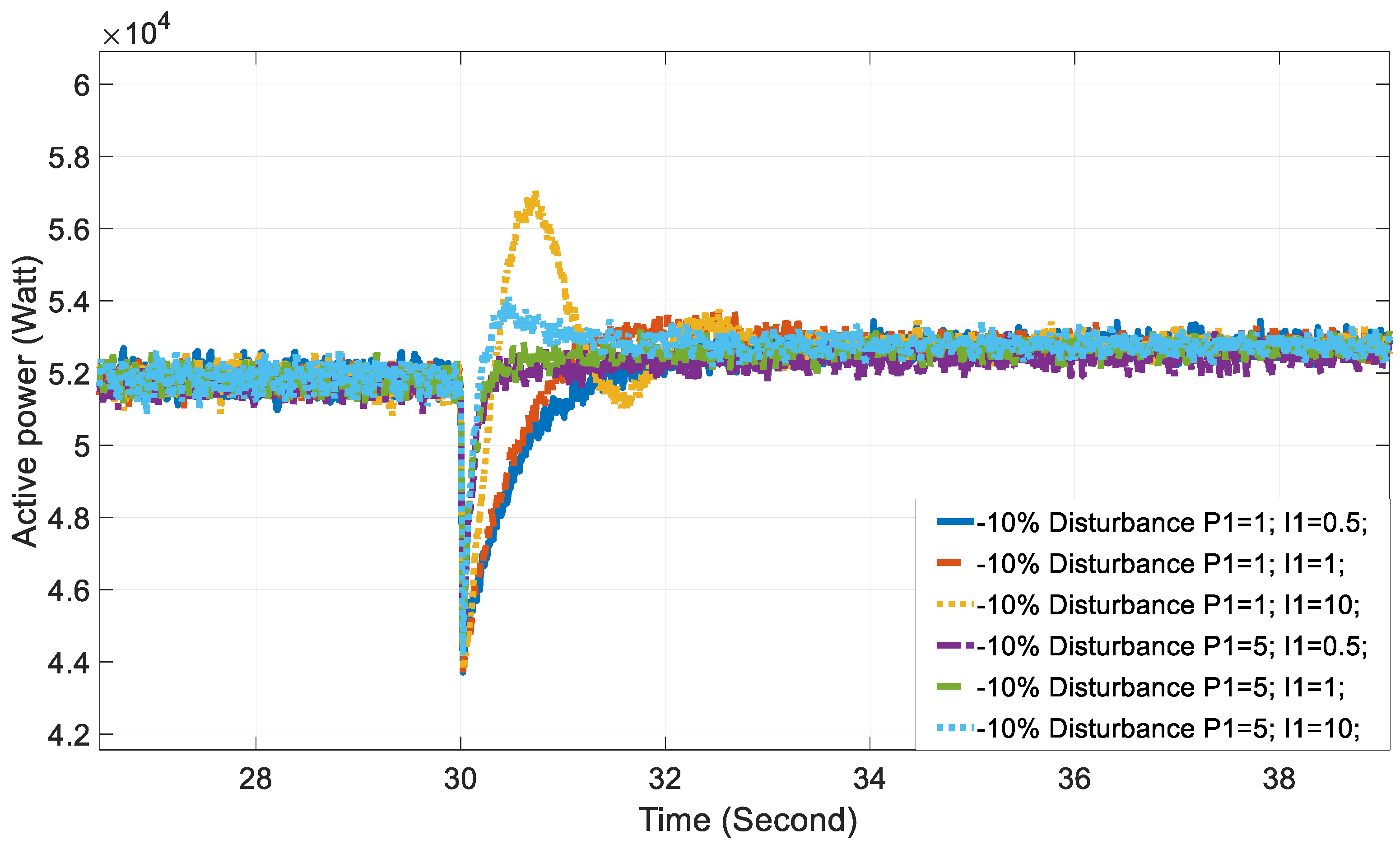
4.4. Dynamic Load Model Parameter for Charging Approach B

In this section, results for the detailed EV model following charging approach B are presented. A similar procedure was followed to highlight that—while in some cases the dynamic response of the detailed EV model could be represented by a standard dynamic load model described by (9)—there were certain cases in which tuning of the PI control parameters led to oscillatory behaviour which could not be properly represented.

In Figure 13, the responses of the detailed EV model—following approach B for different values of the outer voltage loop control parameters (PI1)—are presented. Compared with Figure 9 and Figure 10 (representing the same scenario using approach A), high integral gain led to cases in which oscillatory behaviour began to be observed.

Curve fitting results for such cases are presented in Figure 14, highlighting instances for certain control parameters in which the ability of the standard dynamic load model of (9) was unable to offer a proper fitting or properly represent the dynamic behaviour of an EV charger following charging approach B. The fitted curve of the ERLM reproduced the characteristics of the detailed model well when the integral parameter setting was low (e.g., value of I1 = 0.1). For higher values of the integral parameter, however, ERLM became increasingly unable to represent the dynamic response of the detailed EV charger model. The model began growing oscillatory as the value of the integral gain rose (e.g., I1 = 1). Results from control approach B resembled control approach A. Effectively, larger integral parameters in PI controllers caused higher oscillation and consequently reduced the fitting quality.

Table 4. Dynamic load model parameters for approach B for −15% voltage disturbance.

PI Parameters	${\mathit{A}}_{\mathit{S}}$	${\mathit{A}}_{\mathit{t}}$	${\mathit{T}}_{\mathit{p}}$	R-Squared	NRMSE
$\mathrm{P}1=1; \mathrm{I}1=0.1$	−0.0921	1.312	−0.792	0.9921	0.0118
$\mathrm{P}1=1; \mathrm{I}1=0.5$	−0.0921	1.236	−0.483	0.9661	0.0435
$\mathrm{P}1=1; \mathrm{I}1=1$	−0.0921	1.132	−0.461	0.5689	0.1024

presents the dynamic load model parameters for different integral parameter settings considering the same disturbance. As the integral parameter increased, the value of ${\mathrm{a}}_{\mathrm{t}}$ decreased, implying that the active power transient response amplitude (caused by the transient voltage change) was smaller. Accordingly, the time constant ${\mathrm{T}}_{\mathrm{p}}$ decreased, which indicates a faster recovery time. For large integral settings (i.e., when I1 = 1) the R-squared metric reached a low value of 0.5689, which is an indication of poor fitting quality (i.e., the first-order-based dynamic load model could not adequately describe the observed response).

Compared with the results from charging approach A, the model under charging approach B had a smaller value of ${\mathrm{a}}_{\mathrm{t}}$, indicating a smaller dip in the transient active power response. On the other hand, the system exhibited longer recovery times with higher values for T_p.

Comparing the curve fitting performance from Table 3 and Table 4, approach B had similar (but slightly better) matches (larger R-squared value and smaller NRMSE) for smaller integral settings (i.e., when I1 = 0.1). As the value of the integral parameter increased, Approach B reached smaller values of R-squared and larger NRMSE. This demonstrates that the resulting oscillatory behaviour (under higher integral gains in Approach B) prevented the exponential recovery load model from accurately representing the dynamic behaviour. However, in general, changes in the PI control parameters had similar tendencies and affected the results in a similar manner for both approaches.

5. Conclusions

This paper investigated the performance of a common dynamic load model used in power system studies—specifically, its ability to represent the dynamic behaviour of EVs in response to voltage disturbances. Two detailed EV models were implemented in Matlab/Simulink software, representing two typical charge approaches (slow and fast EV chargers) designated approach A and approach B in this work.

Initially, an analysis of the static behaviour of the detailed models showed a behaviour very close to constant power for both approaches. By applying curve fitting techniques, the static behaviour of both models was fitted to the ZIP and exponential load models. The results showed that static behaviour could be expressed well by standard static load models typically used in power system studies. Static load model parameters for both the ZIP and exponential load models were provided. Furthermore, an investigation of the impact of SoC for both approaches A and B showed that EV chargers exhibited behaviour very close to constant power for different SoCs—and consequently, different internal battery voltages.

The main contribution of this paper was the investigation of the ability of a typical dynamic load model commonly used in dynamic power system studies (the exponential recovery dynamic load model) to represent the dynamic behaviour of two detailed EV models. Curve fitting was used to fit the dynamic load model to the responses from the detailed EV charger models. The results showed that the specific values of control parameters were important; they affected the shape of the dynamic response of the EV chargers. This left standard dynamic load models potentially unable to represent the dynamic behaviour of EV chargers. For both models, certain control parameters (e.g., high proportional or integral PI gains) caused the dynamic behaviour of EV chargers to exhibit oscillatory behaviour which could not be captured in detail by the standard dynamic load model. Representative parameter sets were provided for some cases when the fitting was adequate (i.e., close to the first-order response obtained by the dynamic load model). Such information may be useful to system operators considering how to model the dynamic behaviour of EVs when performing stability studies, as their numbers are increasing. Investigating the magnitude of the potential impact from such differences is also a potential future research direction.

References

1. Bunsen, T.; Cazzola, P.; d’Amore, L.; Gorner, M.; Scheffer, S.; Schuitmaker, R.; Signollet, H.; Tattini, J.; Teter, J. Leonardo Paoli. IEA Technology Report, Global EV Outlook 2019 Scaling up the Transition to Electric Mobility; International Energy Agency: Paris, France, 2019.
2. Arias-Londoño, A.; Montoya, O.D.; Grisales-Noreña, L.F.A. Chronological Literature Review of Electric Vehicle Interactions with Power Distribution Systems. Energies 2020, 13, 3016. [Google Scholar] [CrossRef]
3. Chen, T.; Zhang, X.; Wang, J. A Review on Electric Vehicle Charging Infrastructure Development in the UK. J. Mod. Power Syst. Clean Energy 2020, 8, 193–205. [Google Scholar] [CrossRef]
4. ICF Consulting Services. Overview of Electric Vehicle Market. and the Potential of Points for Demand Response; ICF Consulting Service: Fairfax, VA, USA, 2016; pp. 1–32. [Google Scholar]
5. Lopes, J.A.P.; Soares, F.J.; Almeida, P.M.R. Integration of Electric Vehicles in the Electric Power System. IEEE 2011, 99, 168–183. [Google Scholar] [CrossRef] [Green Version]
6. Garcia-Valle, R.; Lopes, J.A.P. Electric Vehicle Integration into Modern Power Networks; Springer Science & Business Media: New York, NY, USA, 2013; Volume 4, pp. 87–107, 155–203. [Google Scholar] [CrossRef] [Green Version]
7. Chung, Y. Electric Vehicle—Smart Grid Integration Load Modeling, Scheduling and Cyber Security. Ph.D. Thesis, University of California, Los Angeles, CA, USA, 2020. [Google Scholar]
8. Collin, A.J. Advanced Load Modelling for Power System Studies. Ph.D. Thesis, University of Edinburgh, Edinburgh, UK, November 2013. [Google Scholar]
9. Xiao, X.; Molin, H.; Kourtza, P. Component-based modelling of EV battery chargers. In Proceedings of the 2015 IEEE Eindhoven PowerTech, Eindhoven, The Netherlands, 29 June–2 July 2015; pp. 1–6. [Google Scholar] [CrossRef] [Green Version]
10. Dharmakeerthi, C.H.; Mithulananthan, N.; Saha, T.K. Impact of electric vehicle fast charging on power system voltage stability. Int. J. Electr. Power Energy Syst. 2014, 57, 241–249. [Google Scholar] [CrossRef]
11. Singh, B.; Singh, B.N.; Chandra, A.; Al-Haddad, K.; Pandey, A.; Kothari, D.P. A Review of single-phase Improved power quality AC-DC converters. IEEE Trans. Ind. Electron. 2003, 50, 962–981. [Google Scholar] [CrossRef] [Green Version]
12. Qian, K.; Zhou, C.; Allan, M.; Yuan, Y. Modelling of load demand Due to EV Battery Charging in distribution systems. IEEE Trans. Power Syst. 2011, 26, 802–810. [Google Scholar] [CrossRef]
13. Yilmaz, M.; Krein, P.T. Review of charging power levels and infrastructure for plug-in electric and hybrid vehicles. In Proceedings of the 2012 IEEE International Electric Vehicle Conference, Greenville, SC, USA, 4–8 March 2012; Volume 28, pp. 2151–2169. [Google Scholar] [CrossRef]
14. Lin, B.-R.; Hung, T.L.; Huang, C.-H. Bi-directional single-phase half-bridge rectifier for power quality compensation. Electr. Power Appl. IEE Proc. 2003, 150, 397–406. [Google Scholar] [CrossRef]
15. Kempton, W.; Tomic, J. Vehicle-to-grid power fundamentals: Calculating capacity and net revenue. J. Power Sources 2005, 144, 268–279. [Google Scholar] [CrossRef]
16. Kisacikoglu, M.C.; Ozpineci, B.; Tolbert, L.M. EV/PHEV bidirectional charger assessment for V2G reactive power operation. IEEE Trans. Power Electron. 2013, 28, 5717–5727. [Google Scholar] [CrossRef]
17. Tremblay, O.; Dessaint, L.A. Experimental Validation of a Battery Dynamic Model for EV applications. World Electr. Veh. J. 2009, 3, 289–298. [Google Scholar] [CrossRef] [Green Version]
18. Bohn, S.; Agsten, M.; Dubey, A.; Santoso, S. A comparative analysis of PEV charging impacts an international perspective. In SAE Technical Paper; SAE: Detroit, MI, USA, 2015. [Google Scholar] [CrossRef]
19. Khan, W.; Ahmad, A.; Ahmad, F. A comprehensive review of fast charging infrastructure for electric vehicles. Smart Sci. 2018, 6, 256–270. [Google Scholar] [CrossRef]
20. J2954-202010, Ground Vehicle Standard, Wireless Power Transfer for Light-Duty Plug-in/Electric Vehicle and Alignment Methodology; SAE Standard: Warrendale, PA, USA, 2020.
21. Elmhirst, O.; Wagstaff, D.; Grid, N. Forecourt Thoughts: Mass Fast Charging of Electric Vehicles. Bloomberg European Automakers Charge into EV Infrastructure. 2017. Available online: https://global.abb/?aspxerrorpath=/ContentPage.aspx (accessed on 23 March 2021).
22. IEC 62196-3: 2014. Plugs, socket-outlets. In Vehicle Connectors and Vehicle Inlets—Conductive Charging of Electric Vehicles; International Electrotechnical Commission: Geneva, Switzerland, 2014.
23. Kontis, E.O.; Chrysochos, A.I.; Papagiannis, G.K.; Papadopoulos, T.A. Development of measurement-based generic load models for dynamic simulations. In Proceedings of the 2015 IEEE Eindhoven PowerTech, Eindhoven, The Netherlands, 29 June–2 July 2015; pp. 1–6. [Google Scholar] [CrossRef]
24. Karlsson, D.; Hill, D.J. Modeling and identification of nonlinear dynamic loads in power systems. IEEE Trans. Power Syst. 1994, 9, 157–166. [Google Scholar] [CrossRef] [Green Version]
25. Stojanović, D.P.; Korunović, L.M.; Milanović, J.V. Dynamic load modelling based on measurements in medium voltage distribution network. Electr. Power Syst. Res. 2008, 78, 228–238. [Google Scholar] [CrossRef]
26. Kundur, P. Power system load. In Power System Stability and Control; Balu, N.J., Lauby, M.G., Eds.; McGraw-Hill: New York, NY, USA, 1994; pp. 271–312. [Google Scholar]
27. Korunović, L.M.; Milanović, J.V.; Djokic, S.Z.; Yamashita, K.; Villanueva, S.M.; Sterpu, S. Recommended Parameter Values and Ranges of Most Frequently Used Static Load Models. IEEE Trans. Power Syst. 2018, 33, 5923–5934. [Google Scholar] [CrossRef] [Green Version]
28. Bokhari, A.; Alkan, A.; Dogan, R. Experimental determination of the ZIP coefficients for modern residential, commercial, and industrial loads. IEEE Trans. Power Deliv. 2013, 29, 1372–1381. [Google Scholar] [CrossRef]
29. Hill, D.J.; Hiskens, I.A. Dynamic analysis of voltage collapse in power systems. In Proceedings of the 31st IEEE Conference on Decision and Control, Tucson, AZ, USA, 16–18 December 1992; pp. 2904–2909. [Google Scholar]
30. Musavi, F.; Edington, M.; Eberle, W.; Dunford, W.G. Evaluation and Efficiency Comparison of Front End AC-DC Plug-in Hybrid Charger Topologies. IEEE Trans. Smart Grid 2012, 3, 413–421. [Google Scholar] [CrossRef]
31. Kim, J.-S.; Choe, G.-Y.; Jung, H.-M.; Lee, B.-K.; Cho, Y.-J.; Han, K.-B. Design and implementation of a high-efficiency on-board battery charger for electric vehicles with frequency control strategy. In Proceedings of the 2010 IEEE Vehicle Power and Propulsion Conference, Lille, France, 1–3 September 2010; pp. 1–6. [Google Scholar] [CrossRef]
32. Restrepo, M.; Morris, J.; Kazerani, M.; Cañizares, C.A. Modelling and testing of a bidirectional smart charger for distribution system EV integration. IEEE Trans. Smart Grid 2016, 9, 152–162. [Google Scholar] [CrossRef]
33. ABB Terra CE53–JCG. Available online: https://new.abb.com/products/4EPY410071R1/terrace53-cjg-terra-50-kw-charger-ccs-chademo-ac-cable-ce (accessed on 23 March 2021).
34. Delta Electronics, Inc. Delta EV DC Quick Charger for EU. Available online: https://chademo.com/portfolios/delta-electronics1-2/ (accessed on 23 March 2021).
35. Collin, A.; Djokic, S.; Thomas, H.; Meyer, J. Modelling of electric vehicle chargers for power system analysis. In Proceedings of the 11th International Conference on Electrical Power Quality and Utilisation, Lisbon, Portugal, 17–19 October 2011; pp. 1–6. [Google Scholar] [CrossRef]
36. Lee, C.S.; Jeong, J.B.; Lee, B.H.; Hur, J. Study on 1.5 kW battery chargers for neighborhood electric vehicles. In Proceedings of the 2011 IEEE Vehicle Power and Propulsion Conference, Chicago, IL, USA, 6–9 September 2011; pp. 1–4. [Google Scholar] [CrossRef]
37. Horton, R.; Taylor, J.A.; Maitra, A.; Halliwell, J. A time-domain model of a plug-in electric vehicle battery charger. In Proceedings of the 2012 PES T & D, Orlando, FL, USA, 7–10 May 2012; pp. 1–5. [Google Scholar] [CrossRef]
38. Abdelhamid, E.; Abdelsalam, A.K.; Massoud, A.; Ahamed, S. An enhanced performance IPT based battery charger for electric vehicles application. In Proceedings of the 2014 IEEE 23rd International Symposium on Industrial Electronics (ISIE), Istanbul, Turkey, 1–4 June 2014; pp. 1610–1615. [Google Scholar] [CrossRef]
39. Tong, S.; Klein, M.P.; Park, J.W. On-line optimization of battery open circuit voltage for improved state-of-charge and state-of-health estimation. J. Power Sources 2015, 293, 416–428. [Google Scholar] [CrossRef]
40. Marra, F.; Yang, G.Y.; Træholt, C.; Larsen, E.; Rasmussen, C.N.; You, S. Demand profile study of battery electric vehicle under different charging options. In Proceedings of the 2012 IEEE Power and Energy Society General Meeting, San Diego, CA, USA, 22–26 July 2012; pp. 1–7. [Google Scholar] [CrossRef] [Green Version]
Figure 1. Block diagram representation of the exponential recovery load model (ERLM).
Energies 14 01801 g001
Figure 2. Comparison of the fitted curve and the original dynamic response curve for a −15% voltage disturbance happening in the first second; P2 = 10; I2 = 5; P3 = 5; I3 = 10.
Energies 14 01801 g002
Figure 3. Topology for charging approach A (level-2 charge).
Energies 14 01801 g003
Figure 4. Topology for charging approach B (level-3 fast charge).
Energies 14 01801 g004
Figure 5. Simulation & curve fitting results for active power and charging approach A: (a) exponential model, (b) ZIP model.
Energies 14 01801 g005
Figure 6. Simulation & curve fitting results for active power and charging approach B: (a) exponential model, (b) ZIP model.
Energies 14 01801 g006
Figure 7. Active power consumption for different battery equivalent voltage ( E b a t t ) and voltage supplies.
Energies 14 01801 g007
Figure 8. Comparison of dynamic response by different DC/DC PI parameter settings for −5% voltage disturbance (P1 = 1; I1 = 0.1; P2 = 10; I2 = 5).
Energies 14 01801 g008
Figure 9. Dynamic response for the different values of integral gain of PI1 for a −20% voltage disturbance occurring at the 20th second; P2 = 10; I2 = 5; P3 = 5; I3 = 10.
Energies 14 01801 g009
Figure 10. Dynamic response for different proportional gain values of PI1 for a −20% voltage disturbance occuring at the 20th second; P2 = 10; I2 = 5; P3 = 5; I3 = 10.
Energies 14 01801 g010
Figure 11. Dynamic response for control approach A, considering different voltage disturbances (PI settings: P1 = 1; I1 = 10; P2 = 10; I2 = 5; P3 = 5; I3 = 10.
Energies 14 01801 g011
Figure 12. Representative curve fitting results. Comparison of the fitted curve and original response data from charging approach A, considering–15% voltage disturbance (PI control settings: P2 = 10; I2 = 5; P3 = 5; I3 = 10).
Energies 14 01801 g012
Figure 13. Detailed electric vehicle (EV) responses for charging approach B under various PI parameters; setting −10% voltage disturbance happening at t = 30 s (PI setting P2 = 20; I2 = 10; P3 = 1; I3 = 5).
Energies 14 01801 g013
Figure 14. Comparison of the fitted curve and original response data from control approach B, considering −15% voltage disturbance occurring at t = 1 s. Each PI control set as: P2 = 20; I2 = 10; P3 = 1; I3 = 5.
Energies 14 01801 g014