
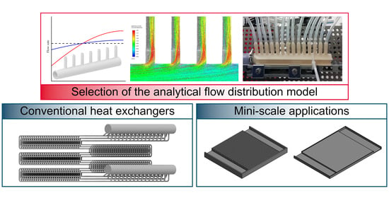
Experimentally Verified Flow Distribution Model for a Composite Modelling System


Abstract
1. Introduction
2. Materials and Methods
- steady-state conditions;
- constant physical properties of the working fluid—water—in the measured temperature range.
2.1. Analytical Models
2.2. CFD Models
- Pressure-based solver with absolute velocity formulation and double-precision;
- Enhanced wall treatment with realizable k–ε model;
- SIMPLE algorithm for pressure–velocity coupling;
- Green–Gauss node based gradient calculation;
- Spatial discretization: second order for pressure, second order upwind for density, momentum, turbulent kinetic energy, and turbulent dissipation rate.
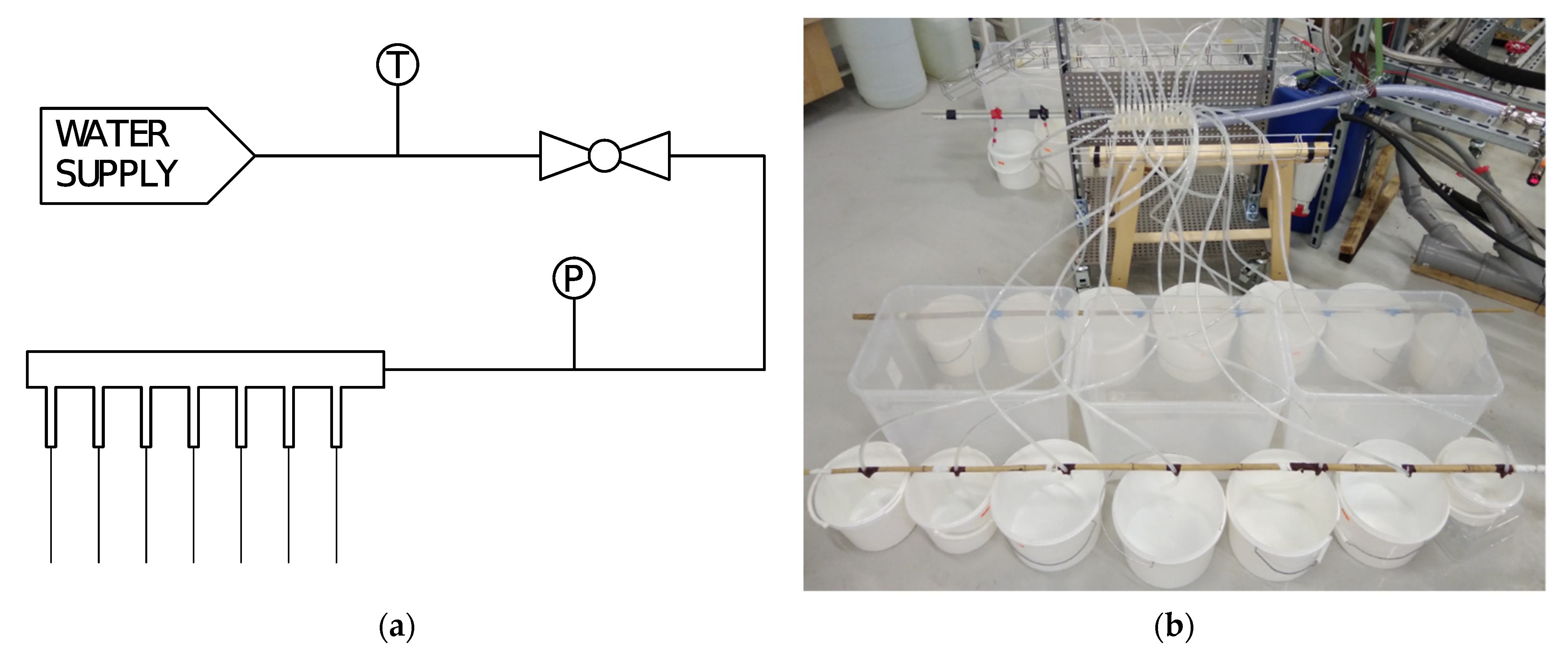
2.3. Experiments
3. Results and Discussion
- One-value criteria provide a single value determining flow maldistribution for the entire system, usually based on flow velocities, mass flow rates, or volumetric flow rates. Examples of such quantification can be the minimum to maximum ratio, ratio of the minimal (maximal) to average value [49], maximum deviation from uniform distribution [50], or relative standard deviation from uniform distribution, to name just a few.
3.1. Results
3.2. Discussion
4. Case Studies
4.1. Minichannel/Minigap Systems
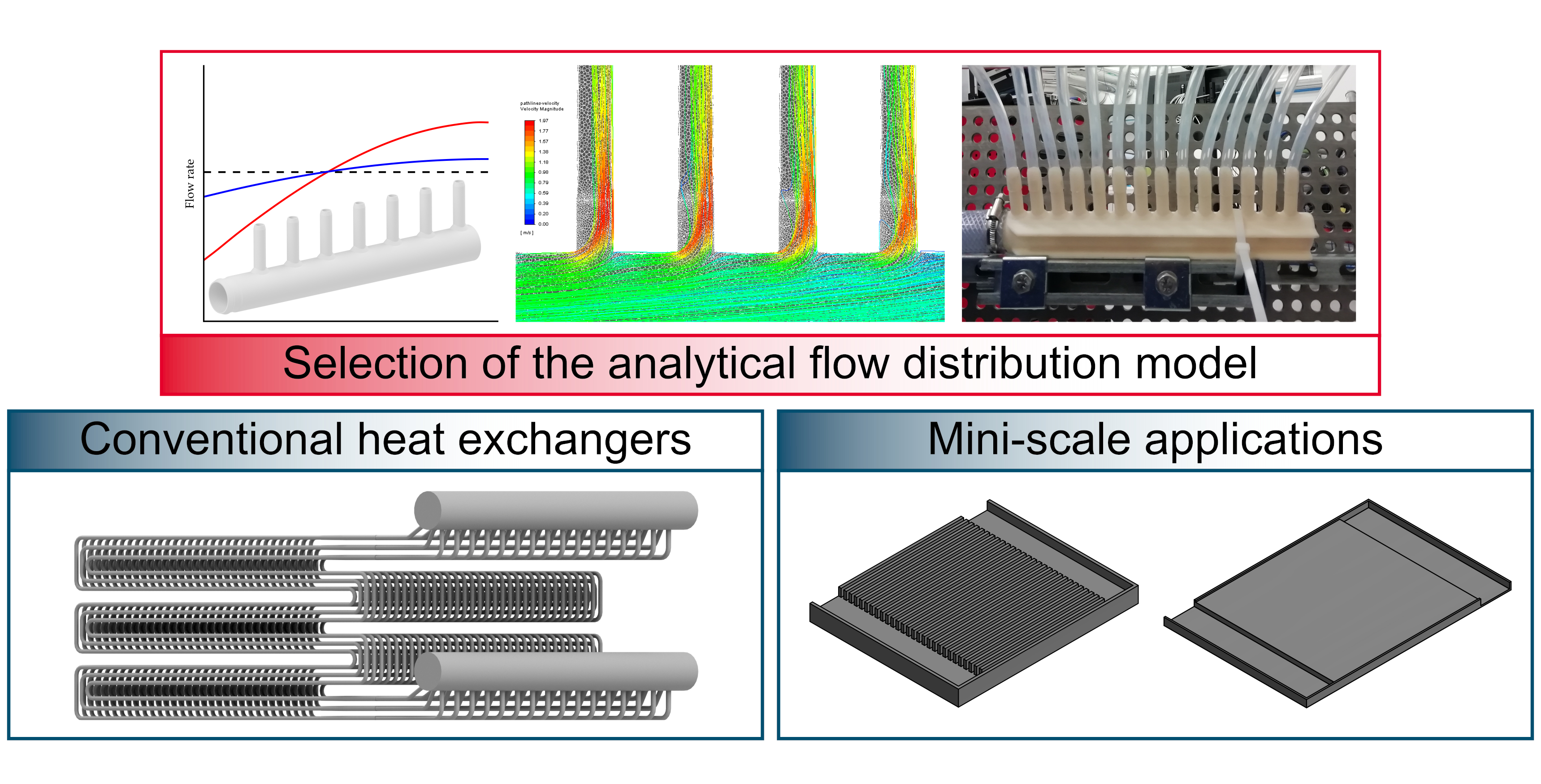
4.2. Industrial Steam Superheater
- The steam superheater is the first convection heat transfer area in the second stage of a boiler in a chemical plant. The apparatus was in a rather unsatisfactory state due to significant discrepancies between design parameters and the actual operating conditions and also because of unsuitable tube material being used. This led to the ruptures of multiple tubes, intensive fouling, and shutdowns of the Y01 and Y03 channels (named after the “Y”-shaped elements dividing each channel into two tubes) [39].
- Only a limited amount of information from the operator of the apparatus was available; therefore, a previous work [54] focused on a CFD simulation of the flue gas flow in the boiler. It should be mentioned that it was not possible to carry out physical experiments that would provide data for verification of the computational model.
- Authors of the present work described in [40] a new methodology of composite modeling that is intended for usage in the initial design of heat transfer equipment. The study [40] also reported drawbacks of modeling simplifications used by commercial software. The distinct advantage of CMS over commercial tools lies in the possibility to easily include data on tube-side fluid flow and, consequently, on more accurate temperature distribution. This can be of vital importance if the equipment is expected to suffer from, e.g., excessive thermal loading due to extreme operating conditions.
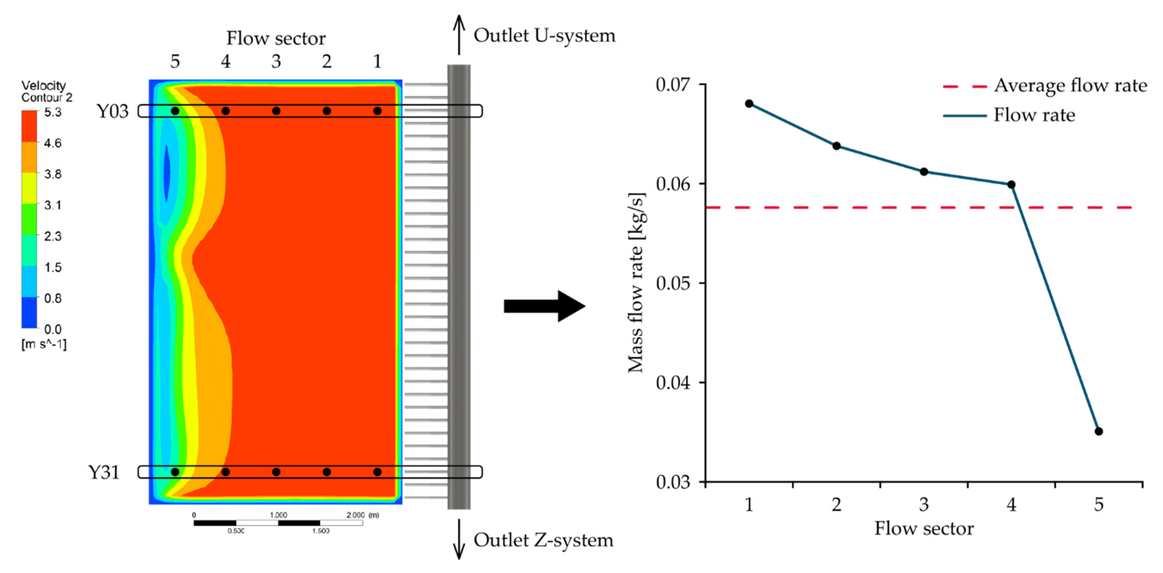
- Flue gas flow (derived from velocity and temperature fields obtained using CFD simulations) was discretized into five streams (Figure 19).
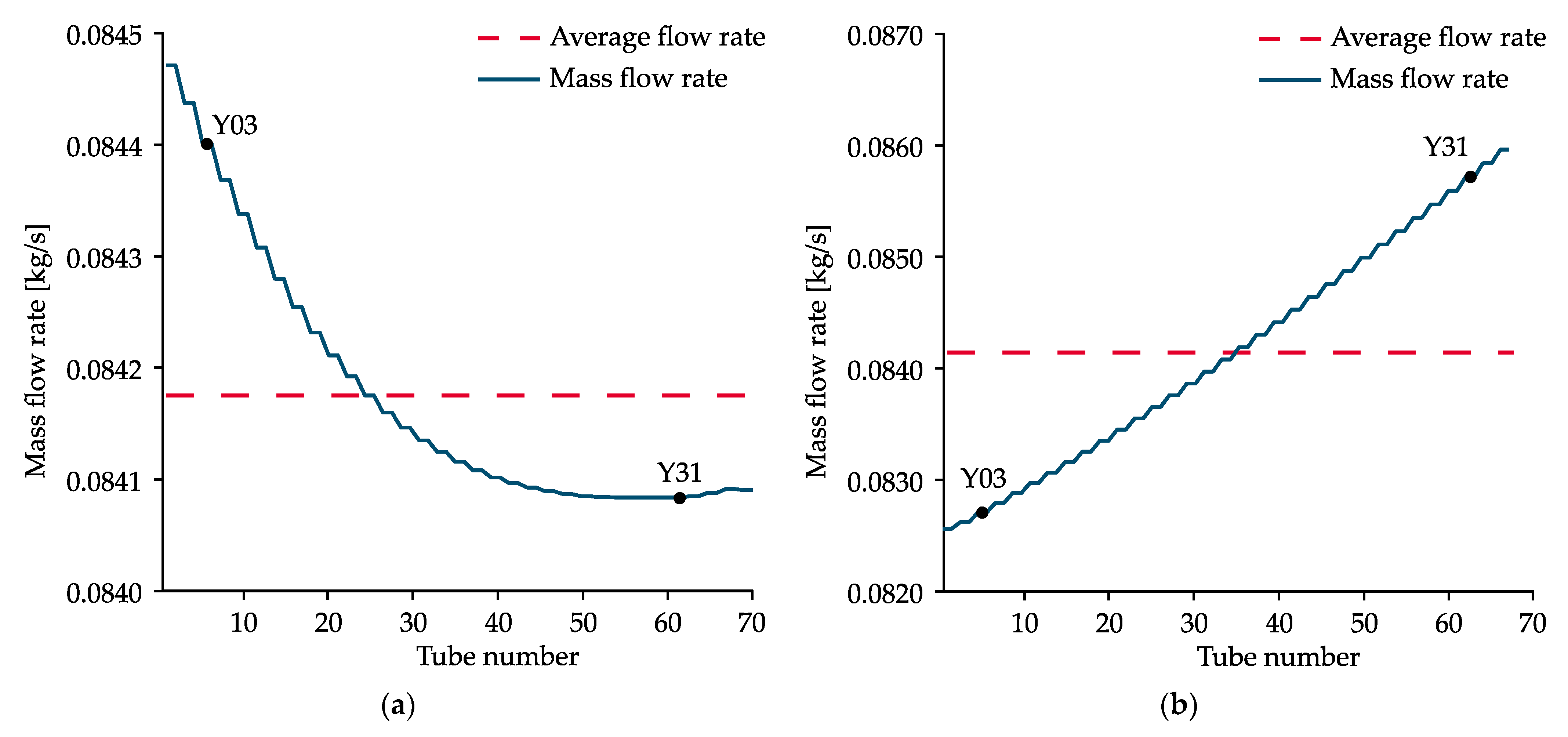
- Superheated steam was divided uniformly in the “Y”-shaped element, i.e., every pair of tubes featured the same flow rate (resulting in a staircase-like shape of the distribution graphs in Figure 20).
5. Conclusions and Future Work
- The modified Model BJ achieved the best fit with experimental data in two modeled configurations with a cross-sectional ratio of ≈0.5 and 2.0. In the case of the basic configuration (Ar of ≈1.0), the model yielded the second closest match. The maximal relative error in the RSD was 8%, which is an acceptable level of accuracy given the extremely low computational time.
- Modifications of Model BJ lay in the adjustment of the momentum coefficient. The best-performing setup was with the momentum coefficient of 1.00 for the distribution system with Ar < 1.0, and with the momentum coefficient of 1.10 for the distribution system with Ar > 1.0. Flow distribution in the basic system was evaluated most accurately when the momentum coefficient attained the value of 1.078, which is higher than the general recommendation (1.05) of the authors of the original model [46].
- As a side effect of the investigation, a notable lack of accuracy was revealed in the maldistribution predictions of steady CFD analyses compared to experimental data. This questions suitability of steady-state data for modeling distribution systems. These inaccuracies, as well as the influence of dynamic flow conditions that were not addressed in this work, will be a part of further research.
- 4.
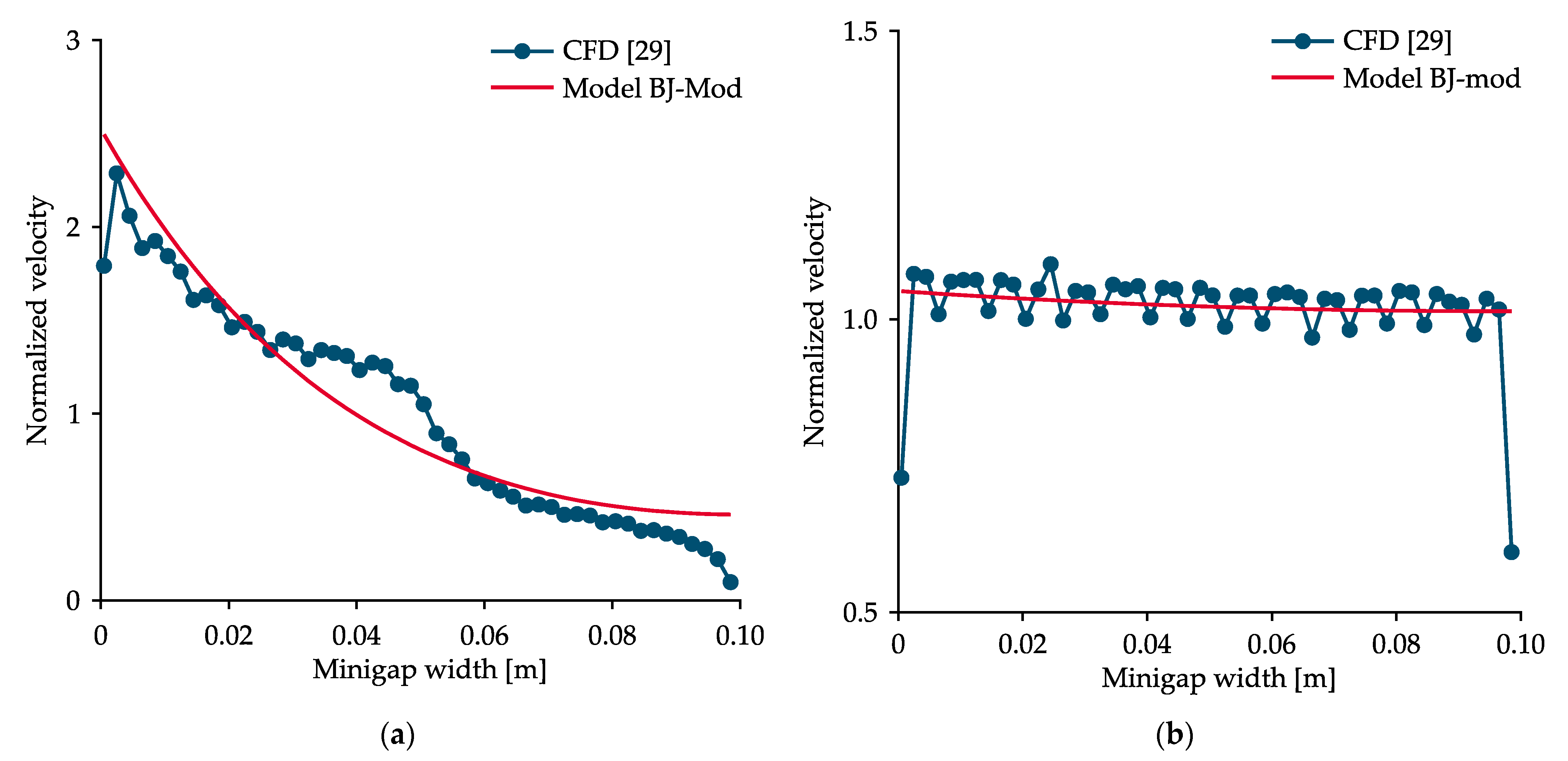
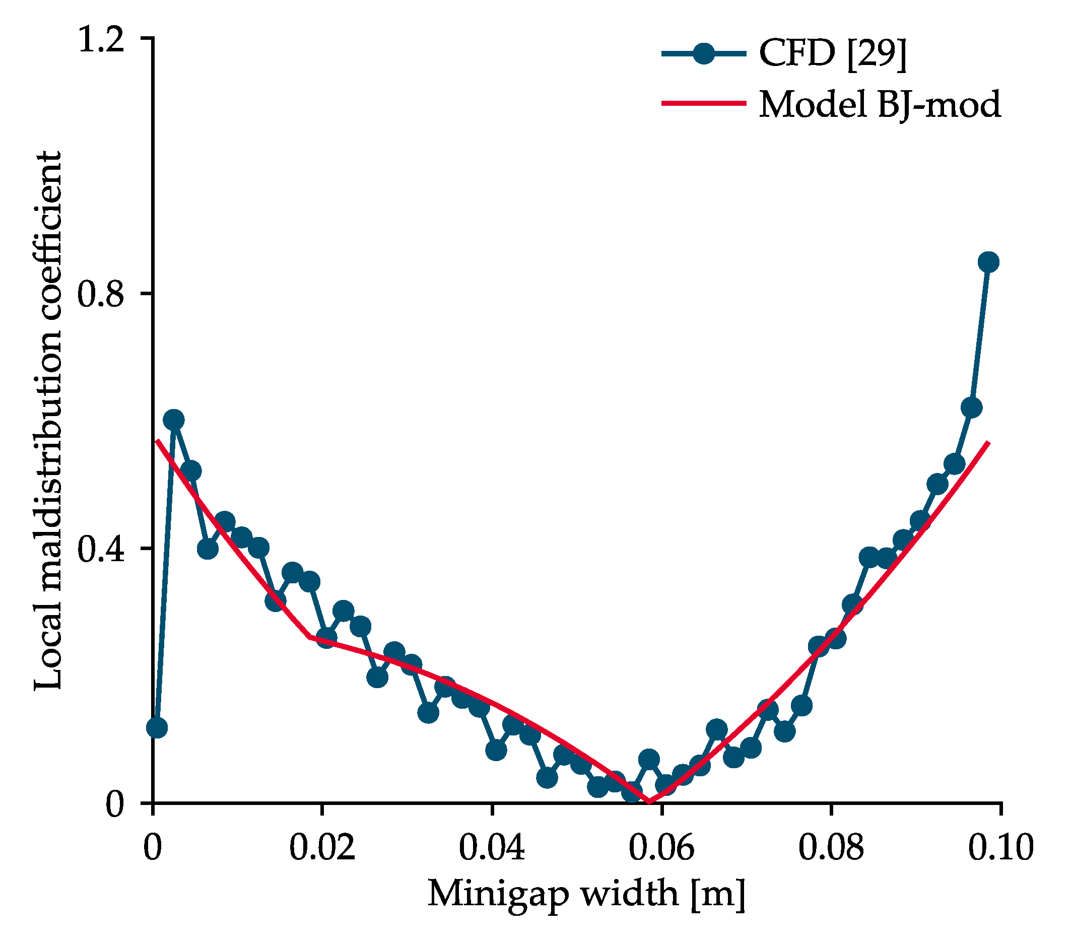
- In minichannel systems, the utilization of modified analytical models is promising, even though the momentum coefficients had to be significantly modified. As for the distributor flow, the best performing momentum coefficient was 0.65 in the most extreme case (Z-arrangement), i.e., almost 40% smaller compared to the mean value recommended for conventional applications. Flow in collectors of both system arrangements was most precisely predicted with the momentum coefficient of 3.10 (approximately 20% larger than recommended). The maximal relative error in the RSD (5%) was observed in the U-system.
- 5.
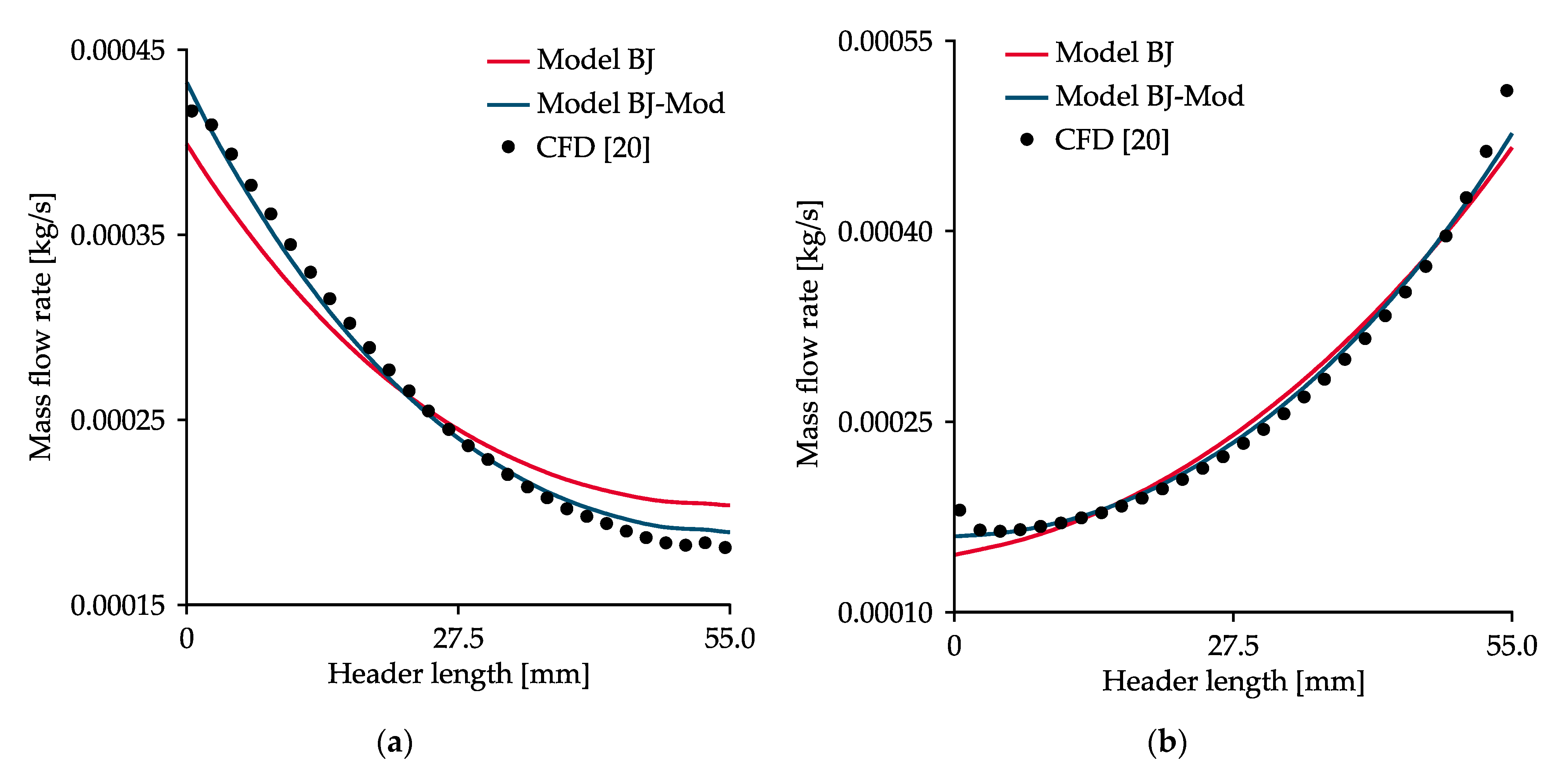
- Usage of analytical models for modeling of rectangular minigaps is limited. However, Model BJ-Mod was at least able to predict the flow non-uniformity trend (up to 5% discrepancy) if the minigap contained deeper headers. On the other hand, no apparent dependence of the momentum coefficients on geometrical parameters was observed.
- 6.
- It can be concluded that low maldistribution affects the performance of equipment only slightly. Moreover, the obtained data showed a significant discrepancy between temperature fields if uniform and non-uniform flow of both process fluids was assumed. The results of the thermal analysis also agreed with the reported operating issues of the respective apparatus.
Author Contributions
Funding
Institutional Review Board Statement
Informed Consent Statement
Data Availability Statement
Acknowledgments
Conflicts of Interest
Nomenclature
| Roman Symbols: | |
| A | cross-sectional area, m2 |
| Ar | cross-sectional ratio, – |
| D | diameter, m |
| f | friction factor, – |
| H | lateral flow resistance, m |
| k | turbulent kinetic energy, m2 s–2 |
| L | length, m |
| L/D | relative header length, – |
| M | momentum change, – |
| MC | local maldistribution coefficient, – |
| n | number, – |
| NU | non-uniformity percentage, % |
| Q | flow rate, m3 s–1 |
| QN | normalized flow rate, – |
| RSD | relative standard deviation, % |
| Rz | roughness of surface, m |
| x | dimensionless distance along the header, – |
| y+ | dimensionless wall distance, – |
| Greek Symbols: | |
| γ | coefficient of static pressure regain, – |
| ε | rate of dissipation of turbulent kinetic energy, m2 s–3 |
| θ | momentum coefficient, – |
| Φ | overall coefficient of friction losses, – |
| ω | specific rate of dissipation of turbulent kinetic energy, s–1 |
| Subscripts: | |
| C | collector flow |
| D | distributor flow |
| i | index of tube or branch |
| id | ideal value |
| T | tube |
References
- Létal, T.; Turek, V.; Babička Fialová, D.; Jegla, Z. Nonlinear finite element analysis-based flow distribution and heat transfer model. Energies 2020, 13, 1664. [Google Scholar] [CrossRef]
- Ocłoń, P.; Łopata, S.; Stelmach, T.; Li, M.; Zhang, J.F.; Mzad, H.; Tao, W.Q. Design optimization of a high-temperature fin-and-tube heat exchanger manifold—A case study. Energy 2021, 215, 119059. [Google Scholar] [CrossRef]
- Kumar, R.; Tiwary, B.; Singh, P.K. Influence of secondary pass location on thermo-fluidic characteristic on the novel air-cooled branched wavy minichannel heat sink: A comprehensive numerical and experimental analysis. Appl. Therm. Eng. 2021, 182, 115994. [Google Scholar] [CrossRef]
- Yih, J.; Wang, H. Experimental characterization of thermal-hydraulic performance of a microchannel heat exchanger for waste heat recovery. Energy Convers. Manag. 2020, 204, 112309. [Google Scholar] [CrossRef]
- Said, S.A.M.; Ben-Mansour, R.; Habib, M.A.; Siddiqui, M.U. Reducing the flow mal-distribution in a heat exchanger. Comput. Fluids 2015, 107, 1–10. [Google Scholar] [CrossRef]
- Gilmore, N.; Hassanzadeh-Barforoushi, A.; Timchenko, V.; Menictas, C. Manifold configurations for uniform flow via topology optimisation and flow visualization. Appl. Therm. Eng. 2021, 183, 116227. [Google Scholar] [CrossRef]
- Anbumeenakshi, C.; Thansekhar, M.R. Experimental investigation of header shape and inlet configuration on flow maldistribution in microchannel. Exp. Therm. Fluid Sci. 2016, 75, 156–161. [Google Scholar] [CrossRef]
- Cho, E.S.; Choi, J.W.; Yoon, J.S.; Kim, M.S. Modeling and simulation on the mass flow distribution in microchannel heat sinks with non-uniform heat flux conditions. Int. J. Heat Mass Transf. 2010, 53, 1341–1348. [Google Scholar] [CrossRef]
- Matheswaran, M.M.; Karthikeyan, S.; Rajiv Kumar, N. Flow distribution analysis in a heat exchanger with different header configurations. ARPN J. Eng. Appl. Sci. 2016, 11, 2812–2817. [Google Scholar]
- Facão, J. Optimization of flow distribution in flat plate solar thermal collectors with riser and header arrangements. Sol. Energy 2015, 120, 104–112. [Google Scholar] [CrossRef]
- Dario, E.R.; Tadrist, L.; Passos, J.C. Review on two-phase flow distribution in parallel channels with macro and micro hydraulic diameters: Main results, analyses, trends. Appl. Therm. Eng. 2013, 59, 316–335. [Google Scholar] [CrossRef]
- Ghani, I.A.; Sidik, N.A.C.; Kamaruzzaman, N.; Yahya, W.J.; Mahian, O. The effect of manifold zone parameters on hydrothermal performance of micro-channel heatsink: A review. Int. J. Heat Mass Transf. 2017, 109, 1143–1161. [Google Scholar] [CrossRef]
- Bava, F.; Furbo, S. A numerical model for pressure drop and flow distribution in a solar collector with U-connected absorber pipes. Sol. Energy 2016, 134, 264–272. [Google Scholar] [CrossRef]
- García-Guendulain, J.M.; Riesco-Ávila, J.M.; Picón-Núñez, M. Reducing thermal imbalances and flow nonuniformity in solar collectors through the selection of free flow area ratio. Energy 2020, 194, 116897. [Google Scholar] [CrossRef]
- Zhengqing, M.; Tongmo, X. Single phase flow characteristics in the headers and connecting tube of parallel tube platen systems. Appl. Therm. Eng. 2006, 26, 396–402. [Google Scholar] [CrossRef]
- Drummond, K.P.; Back, D.; Sinanis, M.D.; Janes, D.B.; Peroulis, D.; Weibel, J.A.; Garimella, S.V. Characterization of hierarchical manifold microchannel heat sink arrays under simultaneous background and hotspot heating conditions. Int. J. Heat Mass Transf. 2018, 126, 1289–1301. [Google Scholar] [CrossRef]
- Pistoresi, C.; Fan, Y.; Aubril, J.; Luo, L. Thermal performances of a multi-scale fluidic network. Appl. Therm. Eng. 2019, 147, 1096–1106. [Google Scholar] [CrossRef]
- Li, H.; Ding, X.; Jing, D.; Xiong, M.; Meng, F. Experimental and numerical investigation of liquid-cooled heat sinks designed by topology optimization. Int. J. Therm. Sci. 2019, 146, 106065. [Google Scholar] [CrossRef]
- Wei, M.; Fan, Y.; Luo, L.; Flamant, G. Design and optimization of baffled fluid distributor for realizing target flow distribution in a tubular solar receiver. Energy 2017, 136, 126–134. [Google Scholar] [CrossRef]
- Kumar, S.; Singh, P.K. A novel approach to manage temperature non-uniformity in minichannel heat sink by using intentional flow maldistribution. Appl. Therm. Eng. 2019, 163, 114403. [Google Scholar] [CrossRef]
- Li, W.; Li, J.; Feng, Z.; Zhou, K.; Wu, Z. Local heat transfer in subcooled flow boiling in a vertical mini-gap channel. Int. J. Heat Mass Transf. 2017, 110, 796–804. [Google Scholar] [CrossRef]
- Piasecka, M.; Musiał, T.; Piasecki, A. Cooling liquid flow boiling heat transfer in an annular minigap with an enhanced wall. EPJ Web Conf. 2019, 213, 1–8. [Google Scholar] [CrossRef]
- Jakubowska, B.; Mikielewicz, D.; Klugmann, M. Experimental study and comparison with predictive methods for flow boiling heat transfer coefficient of HFE7000. Int. J. Heat Mass Transf. 2019, 142, 118307. [Google Scholar] [CrossRef]
- Strak, K.; Piasecka, M. The applicability of heat transfer correlations to flows in minichannels and new correlation for subcooled flow boiling. Int. J. Heat Mass Transf. 2020, 158, 119933. [Google Scholar] [CrossRef]
- Hożejowska, S.; Piasecka, M. Numerical solution of axisymmetric inverse heat conduction problem by the Trefftz method. Energies 2020, 13, 705. [Google Scholar] [CrossRef]
- Klugmann, M.; Dąbrowski, P.; Mikielewicz, D. Flow boiling in minigap in the reversed two-phase thermosiphon loop. Energies 2019, 12, 3368. [Google Scholar] [CrossRef]
- Dąbrowski, P. Thermohydraulic maldistribution reduction in mini heat exchangers. Appl. Therm. Eng. 2020, 173, 115271. [Google Scholar] [CrossRef]
- Klugmann, M.; Dąbrowski, P.; Mikielewicz, D. Flow distribution and heat transfer in minigap and minichannel heat exchangers during flow boiling. Appl. Therm. Eng. 2020, 181, 116034. [Google Scholar] [CrossRef]
- Dąbrowski, P. Mitigation of flow maldistribution in minichannel and minigap heat exchangers by introducing threshold in manifolds. J. Appl. Fluid Mech. 2020, 13, 815–826. [Google Scholar] [CrossRef]
- Zhang, X.; Tiwari, R.; Shooshtari, A.H.; Ohadi, M.M. An additively manufactured metallic manifold-microchannel heat exchanger for high temperature applications. Appl. Therm. Eng. 2018, 143, 899–908. [Google Scholar] [CrossRef]
- Greiciunas, E.; Borman, D.; Summers, J.; Smith, S.J. Experimental and numerical study of the additive layer manufactured inter-layer channel heat exchanger. Appl. Therm. Eng. 2021, 188, 116501. [Google Scholar] [CrossRef]
- Wong, M.; Owena, L.; Sutcliffe, C.J.; Puri, A. Convective heat transfer and pressure losses across novel heat sinks fabricated by Selective Laser Melting. Int. J. Heat Mass Transf. 2009, 52, 281–288. [Google Scholar] [CrossRef]
- Kukulka, D.J.; Smith, R. Thermal-hydraulic performance of Vipertex 1EHT enhanced heat transfer tubes. Appl. Therm. Eng. 2013, 61, 60–66. [Google Scholar] [CrossRef]
- Piasecka, M. Laser texturing, spark erosion and sanding of the surfaces and their practical applications in heat exchange devices. Adv. Mater. Res. 2014, 874, 95–100. [Google Scholar] [CrossRef]
- Li, W.; Tang, W.; Gu, Z.; Guo, Y.; Ma, X.; Minkowycz, W.J.; He, Y.; Kukulka, D.J. Analysis of condensation and evaporation heat transfer inside 3-D enhanced tubes. Numer. Heat Transf. Appl. 2020, 78, 525–540. [Google Scholar] [CrossRef]
- Wei, C.; Vasquez Diaz, G.A.; Wang, K.; Li, P. CFD analysis and evaluation of heat transfer enhancement of internal flow in tubes with 3D-printed complex fins. In Proceedings of the ASME 2019 Heat Transfer Summer Conference collocated with the ASME 2019 13th International Conference on Energy Sustainability, Bellevue, WA, USA, 14–17 July 2019; pp. 1–11. [Google Scholar] [CrossRef]
- Wu, T.; Lee, P.S.; Mathew, J.; Sun, C.; Aw, B.L. Pool boiling heat transfer enhancement with porous fin arrays manufactured by selective laser melting. In Proceedings of the 2019 18th IEEE Intersociety Conference on Thermal and Thermomechanical Phenomena in Electronic Systems (ITherm), Las Vegas, NV, USA, 28–31 May 2019; pp. 1107–1114. [Google Scholar] [CrossRef]
- Turek, V.; Bělohradský, P.; Jegla, Z. Geometry optimization of a gas preheater inlet region—A case study. Chem. Eng. Trans. 2012, 29, 1339–1344. [Google Scholar] [CrossRef]
- Jegla, Z.; Fialová, D. Development of heat and fluid flow distribution modelling system for analysing multiple-distributed designs of process and power equipment. Chem. Eng. Trans. 2018, 70, 1471–1476. [Google Scholar] [CrossRef]
- Fialová, D.; Jegla, Z. Analysis of fired equipment within the framework of low-cost modelling systems. Energies 2019, 12, 520. [Google Scholar] [CrossRef]
- Kilkovský, B. Review of design and modeling of regenerative heat exchangers. Energies 2020, 13, 759. [Google Scholar] [CrossRef]
- Turek, V. New Elements of Heat Transfer Efficiency Improvement in Systems and Units. Ph.D. Thesis, Brno University of Technology, Brno, Czech Republic, 2012. [Google Scholar]
- Fialová, D.; Jegla, Z. Experimental and computational modelling of flow distribution. In Proceedings of the 5th World Congress on Momentum, Heat and Mass Transfer (MHMT’20), Virtual Congress, 14–16 October 2020. ENFHT 148. [Google Scholar] [CrossRef]
- Jones, G.F.; Lior, N. Flow distribution in manifolded solar collectors with negligible buoyancy effects. Sol. Energy 1994, 52, 289–300. [Google Scholar] [CrossRef]
- Bajura, R.A. A model for flow distribution in manifolds. J. Eng. Gas Turb. Power 1971, 93, 7–12. [Google Scholar] [CrossRef]
- Bajura, R.A.; Jones, E.H. Flow distribution manifolds. J. Fluids Eng. 1976, 98, 654–665. [Google Scholar] [CrossRef]
- ANSYS, Inc. ANSYS Fluent User’s Guide, Version 2019 R3; ANSYS, Inc.: Canonsburgh, PA, USA, 2019. [Google Scholar]
- Gandhi, M.S.; Ganguli, A.A.; Joshi, J.B.; Vijayan, P.K. CFD simulation for steam distribution in header and tube assemblies. Chem. Eng. Res. Des. 2012, 90, 487–506. [Google Scholar] [CrossRef]
- Henry, J.A.R. Headers, Nozzles, and Turnarounds. In Heat Exchanger Design Handbook; Hewitt, G.F., Ed.; Begell House: New York, NY, USA, 1998. [Google Scholar]
- Mohammadi, K.; Malayeri, M.R. Parametric study of gross flow maldistribution in a single-pass shell and tube heat exchanger in turbulent regime. Int. J. Heat Fluid Flow 2013, 44, 14–27. [Google Scholar] [CrossRef]
- Fialová, D. Flow Distribution in Equipment with Dense Tube Bundles. Master’s Thesis, Brno University of Technology, Brno, Czech Republic, 2017. (In Czech). [Google Scholar]
- Turek, V.; Fialová, D.; Jegla, Z. Efficient flow modelling in equipment containing porous elements. Chem. Eng. Trans. 2016, 52, 487–492. [Google Scholar] [CrossRef]
- Kumar, R.; Singh, G.; Mikielewicz, S. A new approach for the mitigating of flow maldistribution in parallel microchannel heat sink. J. Heat Transfer 2018, 140, 72401. [Google Scholar] [CrossRef]
- Nad’, M.; Jegla, Z.; Létal, T.; Lošák, P.; Buzík, J. Thermal load non-uniformity estimation for superheater tube bundle damage evaluation. MATEC Web Conf. 2018, 157, 2033:1–2033:10. [Google Scholar] [CrossRef]
- Heat Transfer Research, Inc. HTRI Xchanger Suite User’s Guide, Version 8.0.1; Heat Transfer Research, Inc.: Navasota, TX, USA, 2019. [Google Scholar]


| Coefficient | Model B [45] | Model BJ [46] | Equation Number |
|---|---|---|---|
| Φ1 | fDLD/2DD 1/(ArH) | fDLD/2DD Ar2/H | (2) |
| Φ2 | 0 | 0 | (3) |
| M1 | (2–γD)/H | θDAr2/H | (4) |
| M2 | 0 | 0 | (5) |
| Parameters | Basic Setup | Tested Values | Figures |
|---|---|---|---|
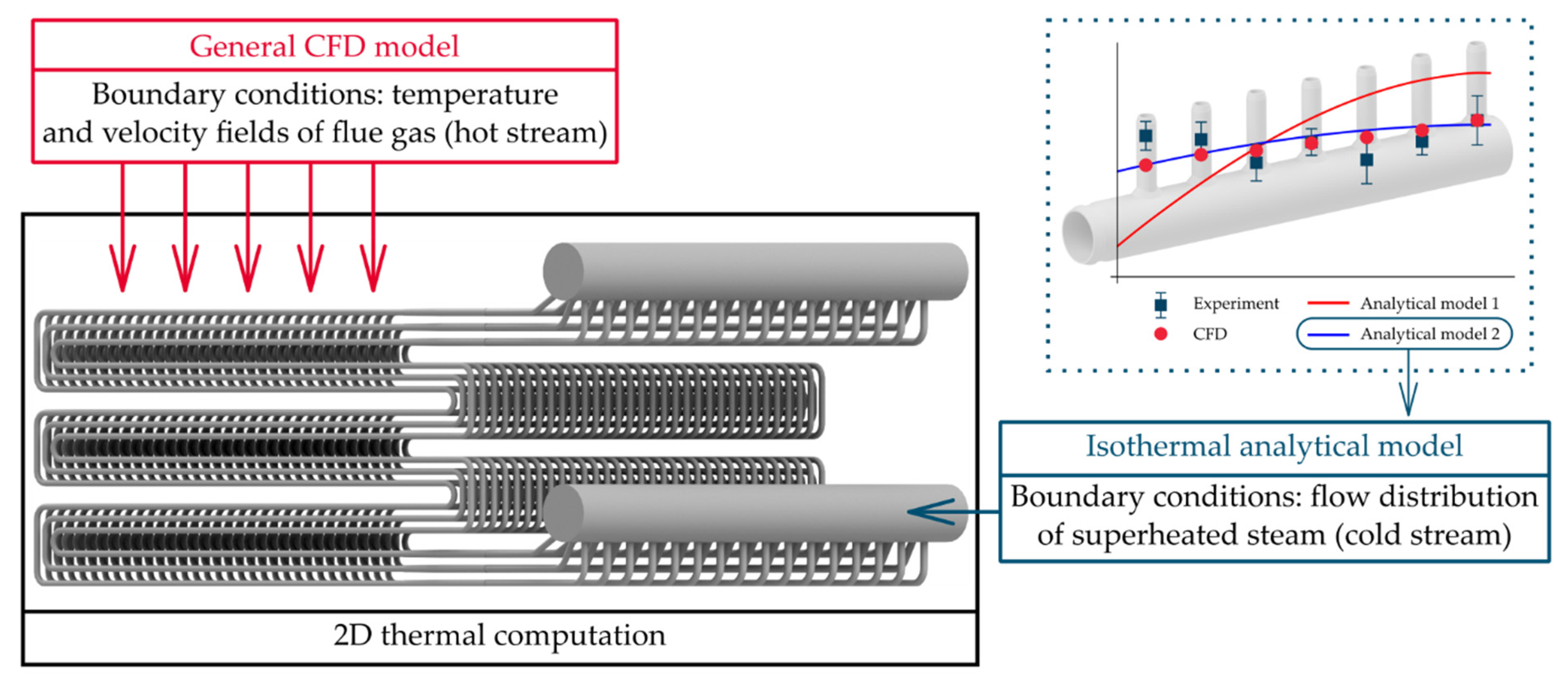
| Header diameter, DD | 0.03 m | ||
| Header length, LD | 0.28 m | ||
| Friction factor, fD | 0.03 | ||
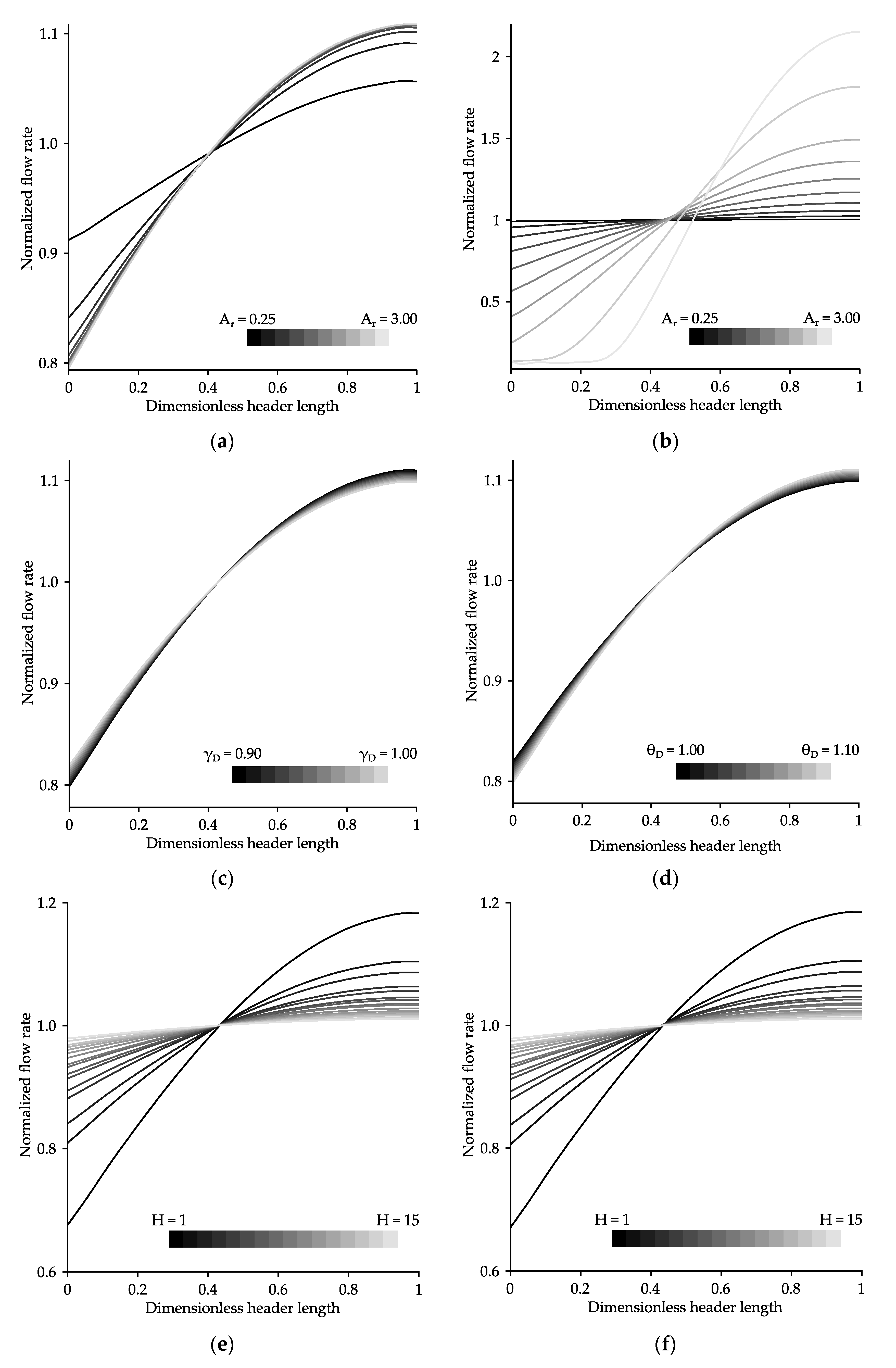
| Cross-sectional ratio, Ar | 1.00 | 0.25, 0.50, 0.75, 1.00, 1.25, 1.50, 1.75, 2.00, 2.50, 3.00 | Figure 5a,b |
| Lateral flow resistance, H | 1.68 m | 1, 1.68, 2, 2.68, 3, 3.68, 4, 4.68, 5, 6, 7, 8, 9, 10, 12.5, 15 | Figure 5e,f |
| Coefficient of static pressure regain, γD | 0.94 | 0.90, 0.91, 0.92, 0.93, 0.94, 0.95, 0.96, 0.97, 0.98, 0.99, 1.00 | Figure 5c |
| Momentum coefficient for header flow, θD | 1.05 | 1.00, 1.01, 1.02, 1.03, 1.04, 1.05, 1.06, 1.07, 1.08, 1.09, 1.10 | Figure 5d |
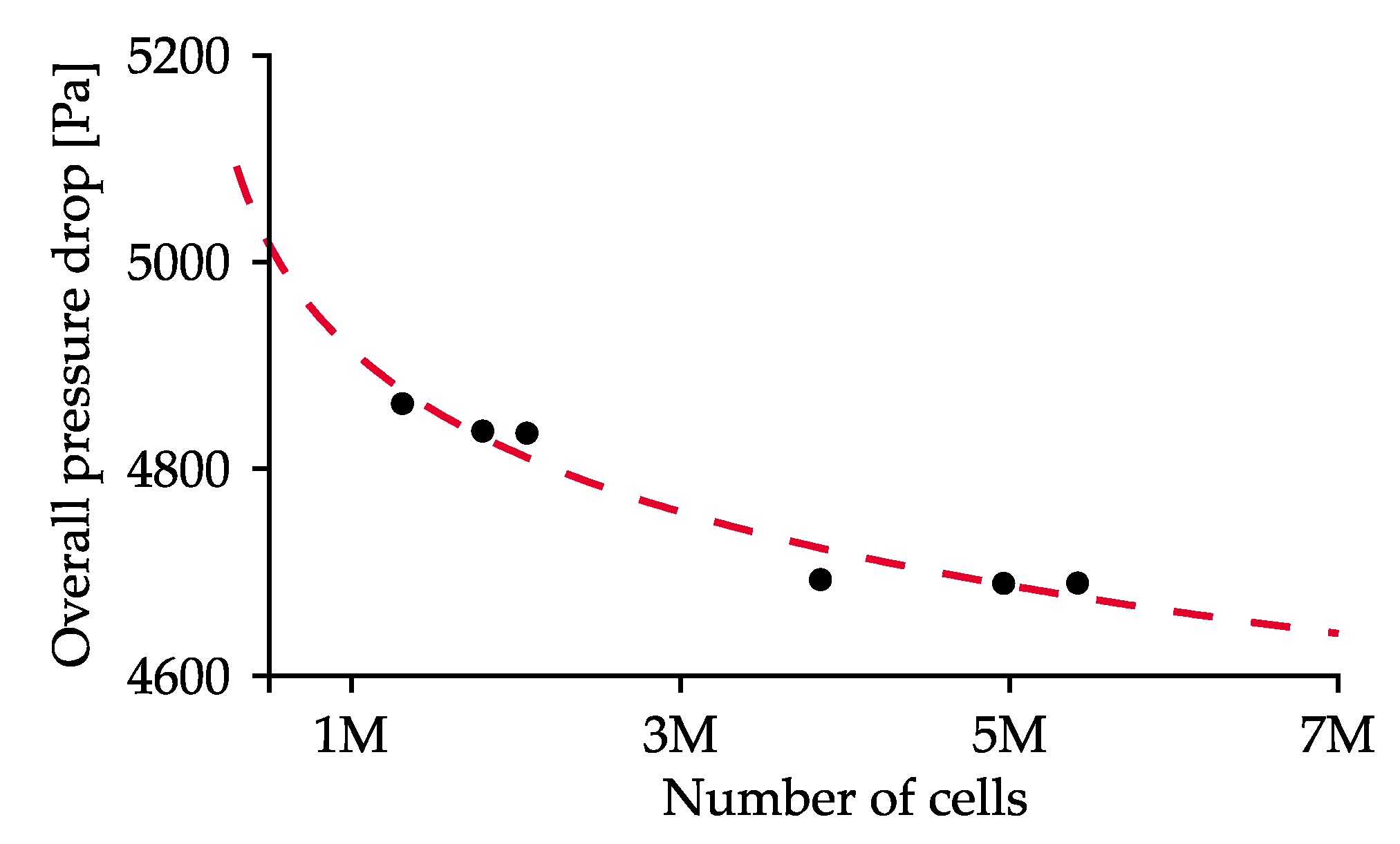
| Mesh | Cell Counts | Min. Orthogonal Quality | Max. Wall y+ 1 | Pressure Drop [Pa] |
|---|---|---|---|---|
| 01 | 1,307,882 | 0.370 | 4.302 | 4856 |
| 02 | 1,798,130 | 0.279 | 3.215 | 4830 |
| 03 | 2,065,477 | 0.229 | 2.471 | 4827 |
| 04 | 3,853,820 | 0.213 | 1.914 | 4686 |
| 05 | 4,964,027 | 0.190 | 1.643 | 4682 |
| 06 | 5,417,477 | 0.126 | 1.138 | 4683 |
| Parameter | Operating Conditions | Measuring Device | Uncertainty |
|---|---|---|---|
| Inlet volumetric flow rate | 42.04–68.83 L/min | IFM SM 8000 | ±1.06 L/min |
| Temperature of water | 17.86–20.75 °C | Sensit PTS 360 | ±0.40 °C |
| Water pressure | 53.39–249.10 kPa (g) | IFM PN 2594 | ±2.00 kPa |
| Ambient pressure | 97.31–99.33 kPa | COMET T2114 | ±0.15 kPa |
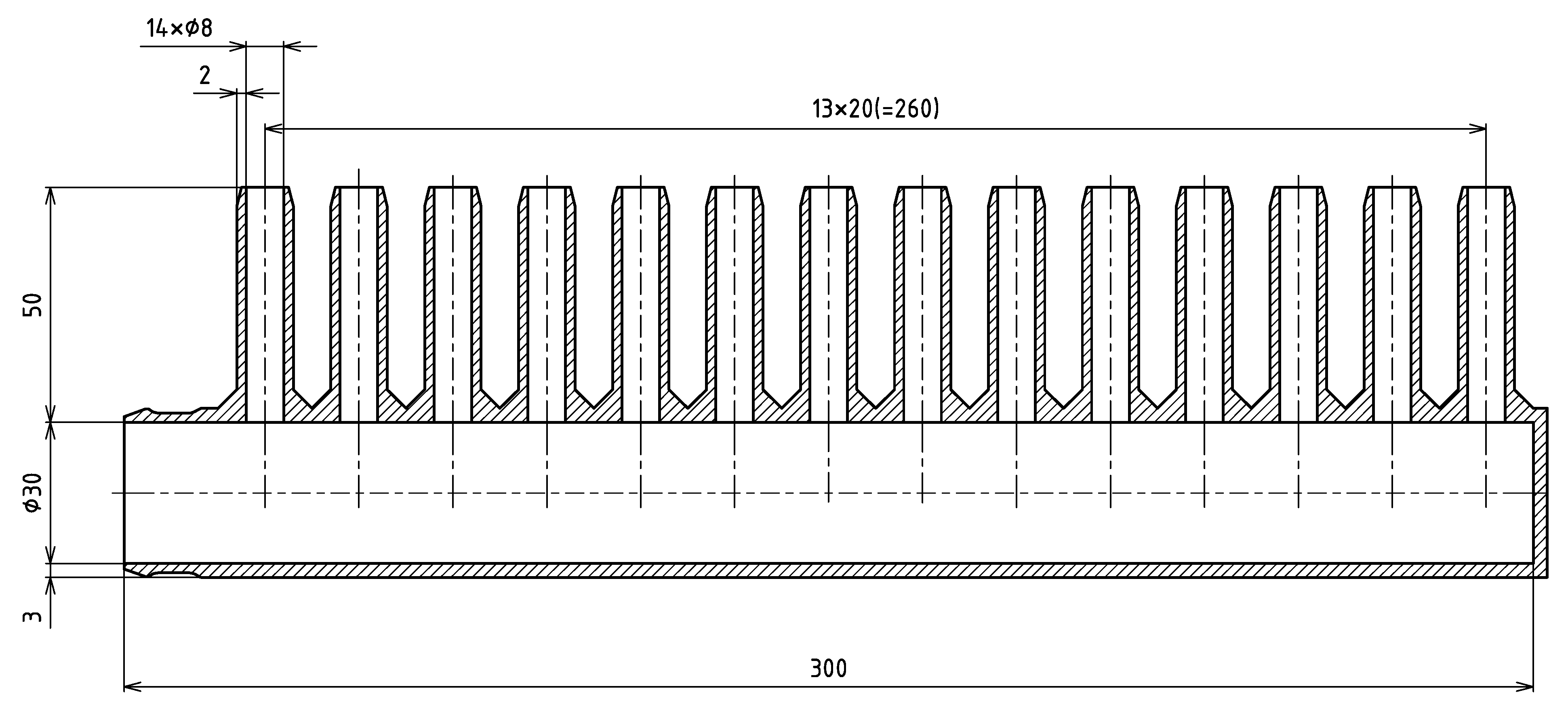
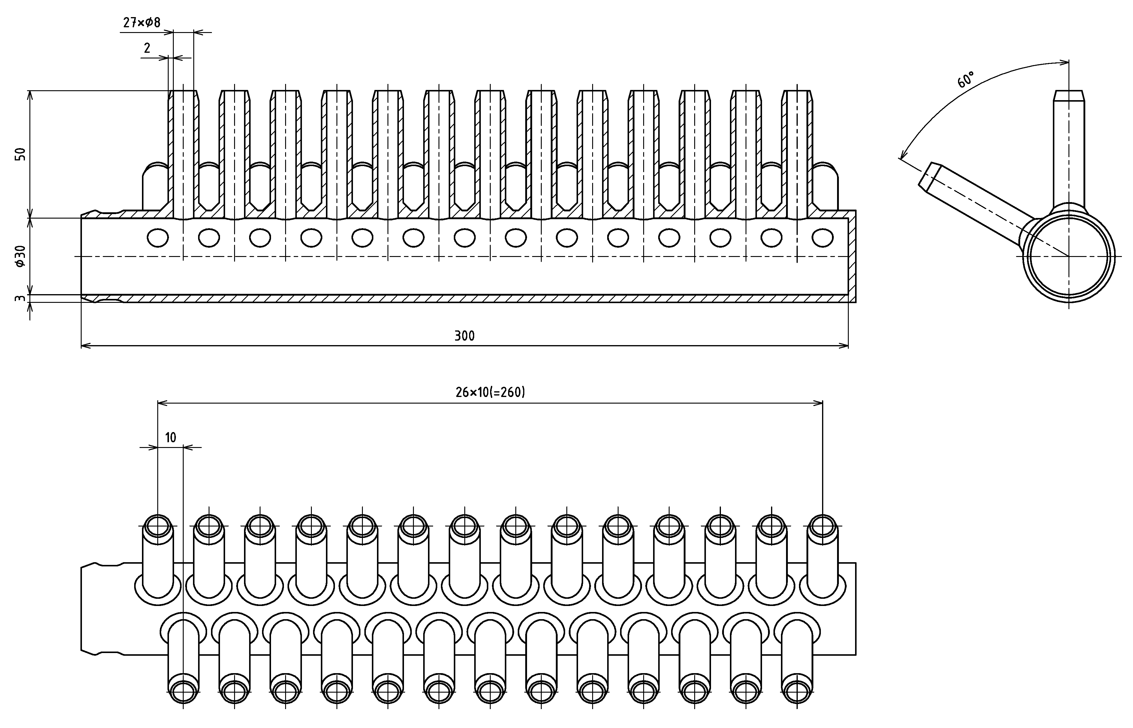
| Parameters | n07 | n14 | n27 |
|---|---|---|---|
| Relative header length | 10 | 10 | 10 |
| Tube pitch | 40 mm | 20 mm | 10 mm |
| Friction factor in the header | 0.028 | 0.028 | 0.026 |
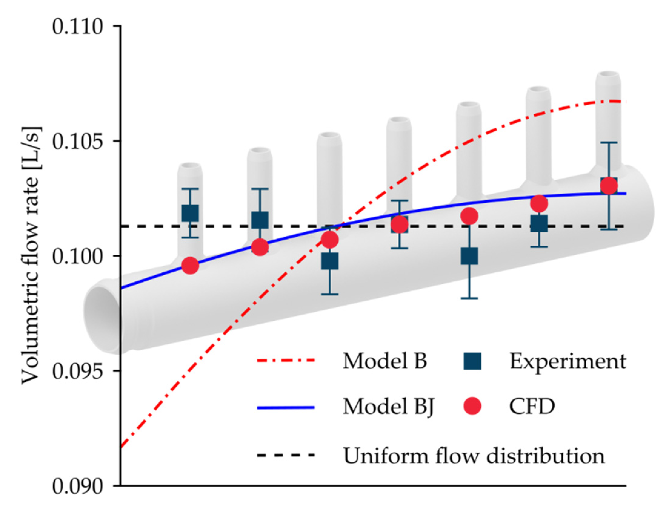
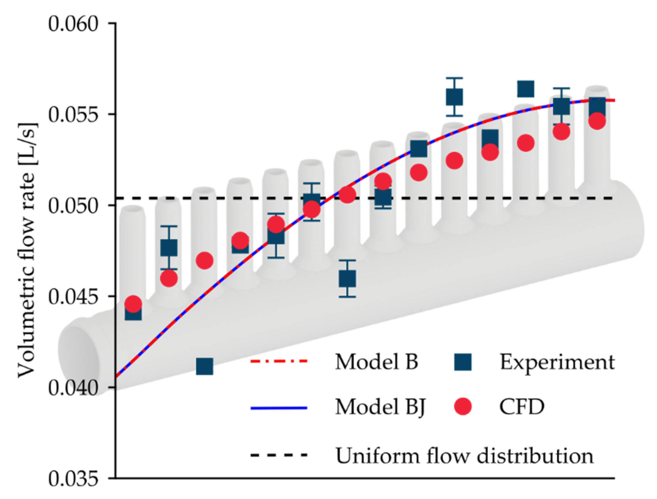
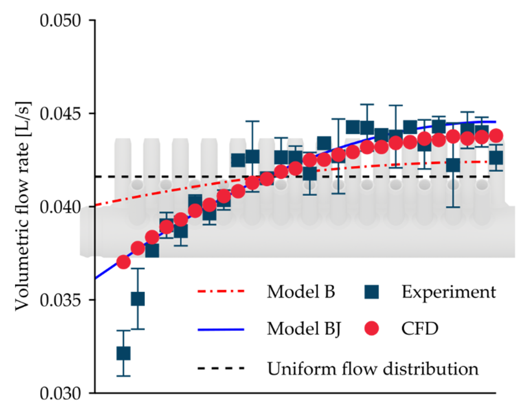
| Cross-sectional ratio | 0.498 | 0.996 | 1.920 |
| Lateral flow resistance | 2.78 m | 1.68 m | 1.71 m |
| Coefficient of static pressure regain (best fitting/default value) | 1.00/0.94 | 0.93/0.94 | 0.90/0.94 |
| Momentum coefficient for header flow (best fitting/default value) | 1.00/1.05 | 1.078/1.050 | 1.10/1.05 |
| Inlet volumetric flow rate | 0.709 L/s | 0.705 L/s | 1.123 L/s |
| n07 | n14 | n27 | ||||||||||
|---|---|---|---|---|---|---|---|---|---|---|---|---|
| Modeling Approach | B | BJ | CFD | E | B | BJ | CFD | E | B | BJ | CFD | E |
| RSD [%] | 4.078 | 1.087 | 1.079 | 1.018 | 9.138 | 9.134 | 5.975 | 9.135 | 1.526 | 5.583 | 4.831 | 7.070 |
| NU [%] | 10.932 | 3.028 | 3.372 | 3.170 | 25.633 | 25.628 | 18.407 | 27.019 | 4.754 | 16.490 | 15.468 | 27.436 |
| Max. rel. difference of flow rate [%] | −6.670 | 2.288 | −2.233 | - | 10.935 | 10.937 | 14.132 | - | 25.677 | 15.748 | 15.228 | - |
| Validation CFD Data [20] | Model BJ | Model BJ-Mod | ||||
|---|---|---|---|---|---|---|
| Arrangement | U | Z | U | Z | U | Z |
| RSD [%] | 28.64 | 37.34 | 21.92 | 36.31 | 27.19 | 36.08 |
| NU [%] | 56.61 | 67.91 | 48.36 | 68.28 | 55.62 | 65.99 |
| Max. rel. difference of flow rate [%] | - | - | 12.71 | −19.07 | 4.91 | −11.31 |
| Modeling Approach | Flue Gas Temperature [°C] | Steam Temperature [°C] | Heat Duty [W] | Effectiveness [%] | |||
|---|---|---|---|---|---|---|---|
| Inlet | Outlet | Inlet | Outlet | ||||
| HTRI | uniform flow | 734.00 | 495.52 | 248.20 | 369.02 | 83,417 | 49.09 |
| CMS | uniform flow | 734.00 | 497.53 | 248.20 | 368.18 | 82,665 | 48.68 |
| CMS | U-system Y03 | 754.76 | 504.46 | 248.20 | 369.23 | 83,429 | 47.25 |
| U-system Y31 | 731.92 | 503.40 | 248.20 | 369.30 | 83,273 | 47.46 | |
| Z-system Y03 | 754.76 | 505.55 | 248.20 | 371.44 | 83,172 | 47.23 | |
| Z-system Y31 | 731.92 | 502.85 | 248.20 | 367.03 | 83,466 | 47.58 | |
Publisher’s Note: MDPI stays neutral with regard to jurisdictional claims in published maps and institutional affiliations. |
© 2021 by the authors. Licensee MDPI, Basel, Switzerland. This article is an open access article distributed under the terms and conditions of the Creative Commons Attribution (CC BY) license (http://creativecommons.org/licenses/by/4.0/).
Share and Cite
Fialová, D.B.; Jegla, Z. Experimentally Verified Flow Distribution Model for a Composite Modelling System. Energies 2021, 14, 1778. https://doi.org/10.3390/en14061778
Fialová DB, Jegla Z. Experimentally Verified Flow Distribution Model for a Composite Modelling System. Energies. 2021; 14(6):1778. https://doi.org/10.3390/en14061778
Chicago/Turabian StyleFialová, Dominika Babička, and Zdeněk Jegla. 2021. "Experimentally Verified Flow Distribution Model for a Composite Modelling System" Energies 14, no. 6: 1778. https://doi.org/10.3390/en14061778
APA StyleFialová, D. B., & Jegla, Z. (2021). Experimentally Verified Flow Distribution Model for a Composite Modelling System. Energies, 14(6), 1778. https://doi.org/10.3390/en14061778