Article

A Quadratically Constrained Optimization Problem for Determining the Optimal Nominal Power of a PV System in Net-Metering Model: A Case Study for Croatia

Department of Energy and Power Systems, Faculty of Electrical Engineering and Computing, University of Zagreb, Unska 3, 10000 Zagreb, Croatia
*
Author to whom correspondence should be addressed.
Energies 2021, 14(6), 1746; https://doi.org/10.3390/en14061746
Submission received: 16 February 2021 / Revised: 17 March 2021 / Accepted: 18 March 2021 / Published: 21 March 2021

Abstract

:
The world’s demand for electrical energy is increasing rapidly while the use of fossil fuels is getting limited more and more by energy policies and the need for reducing the impact of climate change. New sources of energy are required to fulfill the world’s demand for electricity and they are currently found in renewable sources of energy, especially in solar and wind power. Choosing the optimal PV nominal power minimizes the unnecessary surplus of electrical energy that is exported to the grid and thus is not making any impact on the grid more than necessary. Oversizing the PV system according to the Croatian net-metering model results in switching the calculation of the costs to the prosumer model which results in a decrease of the project’s net present value (NPV) and an increase in the payback period (PP). This paper focuses on formulating and solving the optimization problem for determining the optimal nominal power of a grid-connected PV system with a case study for Croatia using multiple scenarios in the variability of electricity production and consumption. In this paper, PV systems are simulated in the power range that corresponds to a typical annual high-tariff consumption in Croatian households. Choosing the optimal power of the PV system maximizes the investor’s NPV of the project as well as savings on the electricity costs. The PP is also minimized and is determined by the PV production, household consumption, discount rate, and geographic location. The optimization problem is classified as a quadratically constrained discrete optimization problem, where the value of the optimal PV power is not a continuous variable because the PV power changes with a step of one PV panel power. Modeling and simulations are implemented in Python using the Gurobi optimization solver.

1. Introduction

In today’s society where technology keeps developing rapidly and the human population and its needs keep increasing simultaneously, the demand for electrical energy also keeps rising significantly. Because of the negative impact of fossil fuels on the Earth’s climate and the ecosystem due to the emission of greenhouse gases, the world seeks its energy sources alternatively. Renewable energy sources (RES) have found their place in the energy transition and decarbonization [1]. Their zero-emission of greenhouse gases and their zero cost of fuel makes them nearly ideal for decarbonization of the energy sector and competition on the market. The share of renewables in the total electricity production is increasing rapidly, both in developed and developing countries [2]. According to [2], RES can be separated into two main groups: dispatchable technologies (biomass, concentrated solar power with storage, geothermal power, and hydropower) and non-dispatchable, also known as variable renewable energy (VRE) (i.e., solar PV, wind power, and ocean power). VRE technologies have four distinctive characteristics: variability—due to the temporal availability of resources, uncertainty—due to the unexpected changes in resource availability, location-specific properties—due to the geographical availability of resources, and low marginal costs—due to freely available resources [2].
At first, power systems were designed and built to operate according to a model that set all of the production (thermal, hydro, and nuclear) on the transmission side of the grid and consumption to the distribution side of the grid. This type of design makes power flows unidirectional, which means that the flow of energy is going from the transmission grid into the distribution grid where it is consumed and each electrical component of the power system is designed according to that direction of power flow (power lines, transformers, protection devices, etc.). The grid operation can be maintained in the safety margins by regulating the output power of the power plants, where the production is following the consumption pattern. This paradigm changes significantly as the penetration of RES into the grid increases. With RES, there is no more “production follows the pattern of consumption” paradigm. The production pattern of RES is not as predictable and controllable as the production of conventional power plants (thermal, hydro, and nuclear). Wind and solar production have a more stochastic nature which makes engineers seek for new solutions to maintain the grid’s stability. Due to their intermittent characteristic, solar and wind RES are not able to be baseload power plants, such as fossil, thermal, or nuclear power plants. Regarding the stochastic nature of wind production, the authors in [3] state that sudden changes in wind power may negatively affect the power system, as well as increase the costs associated with maintaining the desired system reliability level and the need for providing the ancillary services to balance the grid. Furthermore, it is stated that these negative effects can be reduced using the geographical diversification of wind power generators technique which is making the network safer and more reliable. Namely, the portfolio theory points out that merging two independent or negatively correlated stochastic properties reduces the portfolio’s variability and enables a more predictable outcome. Basically, treating a set of wind power stations as one virtual station, an increase in geographical dispersion leads to a reduction of variability in output power making the virtual station similar to the baseload production.
According to [2], the integration of a significant amount of variable renewables into the power grid requires certain actions to increase the flexibility of the existing grid: (a) electricity flow has to be allowed, not only from centralized power plants to users but also from micro-prosumers to the grid, which is aimed to ensure grid stability when installing distributed generation; (b) smart grid and demand management models aimed at increasing the flexibility and responsiveness and reducing peak-loads to deal with increased variability have to be established; (c) improving grid interconnection at the regional and international level aimed at increasing balancing capabilities, flexibility, stability, and security of supply is a must; (d) introducing energy storage capacity to store electricity (energy) from variable renewables generation when production exceeds demand. In [4] the concept of virtual point of connection (VPC) is introduced to eliminate the restriction for accessing the power grid by the current physical point of connection (PPC). Namely, the authors state that the idea of non-restricted use of low voltage (LV) networks by electricity consumers and prosumers should enable the significant development of electromobility as well as have a positive impact on future expansion of distributed energy sources (RES) in prosumer micro-installations. The concept of VPC is especially suitable for LV networks in the form of clusters or energy clouds, where the participants should experience the ease of use of the network in mentioned structures, as stated in [4]. The increase of prosumer micro-installations can also be one of the solutions for tackling the current problem of greenhouse gas emissions [5]. Furthermore, the development of the prosumer micro-installations increases the level of energy security since the energy sources have an increased energy diversification and are widely dispersed across the country. Due to the economies of scale, as well as the growing technological maturity of micro-installations, capital costs of the projects decrease as well as the costs of electricity after the installation. Consequently, households and companies are becoming more motivated to become RES prosumers [5].
One of the main ideas and solutions for tackling the RES stochastic and intermittent nature are forecasting models that use machine and deep learning algorithms to minimize their errors. These types of forecasting algorithms enable the grid operator to see the future production of RES with high accuracy and thus enable it to act in time according to the change of the parameters in the grid. Such artificial intelligence models can also be used to forecast electrical energy prices on the spot market or even forecast the carbon prices in real-time, as stated in [6].
Distributed production of RES is also making a change in the grid. Primarily, distributed production of RES is increasing the voltage level at certain points in the distribution network, as well as changing the direction of the power flow making the flow bidirectional [7]. Installing the optimal nominal power of a certain RES power plant minimizes the impact on the grid.
In [8], the author uses the HOMER software to determine the optimal nominal power of a PV system by minimizing the COE (cost of energy) in a net-metering model. Furthermore, the author states that the system uses battery storage as a backup source which increases the COE. Contrary to [8], this paper uses a grid-connected PV system only, without battery storage. However, the objective function in this paper is not minimizing the COE directly, but rather minimizing the difference of imported and exported electricity (difference in power flow) on an annual basis, with regards to all technical, economic, and legal constraints, as well as considering the variability on the production and consumption side. In [9], the two approaches for determining the optimal nominal power of a PV system under the net-metering model are proposed: a deterministic and a stochastic approach. On the one hand, the deterministic approach uses all of the available and known input variables with certainty and aims to match the expected demand with the estimated PV production. On the other hand, with the stochastic approach, the author uses PSO (particle swarm optimization) to determine the most likely optimal sizing of the system which matches the consumption needs, while the uncertainty variables are randomly modeled using the probability distributions within the Monte Carlo (MC) algorithm. In this paper, similarly as in [9] where the author uses minimization of the net power flow at a meter (considering MC simulation every hour) as an objective function, the objective function is a minimization of the net power flow on an annual basis.
The objective of this paper is to model and determine the optimal nominal powers of the PV systems for a multiple scenarios case study for the cities of Zagreb and Split in Croatia. Split is considered to be the representative city for the Mediterranean region of Croatia, while Zagreb is considered to be the representative city for the continental region of Croatia. In this paper, household micro-PV systems are modeled with the nominal power ranging from 2.1 to 6 kWp. Solar PV systems are grid-connected and are in the net-metering model. The optimization problem has been formulated in Python and solved using a Gurobi solver. Technical constraints of PV systems have been considered as well as the constraints regarding the implementation of the net-metering model. Simulation has been conducted for multiple scenarios of Zagreb and Split with consideration of the variability of household consumption and PV production on an annual basis. In addition, an overview of the solar PV market models as a comparison between certain EU countries is presented. The optimization algorithm and simulation results with comparison analysis will be presented in the following chapters.

2. PV Market Models

There are currently a lot of market models that support RES in the EU. The most popular ones, especially for solar PV, are variations of the feed-in tariff (FiT), the net-metering model, and the latest feed-in premium model.
To have a better visual representation of the FiT and net-metering models, production and consumption profiles of an average household in Zagreb have been modeled as well as the energy balance (energy flow from and to the grid) for an average day in August. Statistically processing hourly data obtained by the energy meter (obtained from research associated with Croatian electrical energy suppliers), the load profile curve has been modeled for an average day in August. Regarding the PV production, an average curve of a typical day in August for insolation has been obtained from [10]. Typical daily profiles for August are shown in Figure 1.
As can be seen in Figure 1a, the mean values for the hours in a day for all days throughout August have been lifted due to the strong influence of outliers (empty circles), while the outliers have much less impact on the median values. Nevertheless, an average daily curve for August has been modeled using the mean values from the dataset. Figure 1b was created using the parameters of south orientation, fixed panels at 35°, and location of Zagreb as input values.

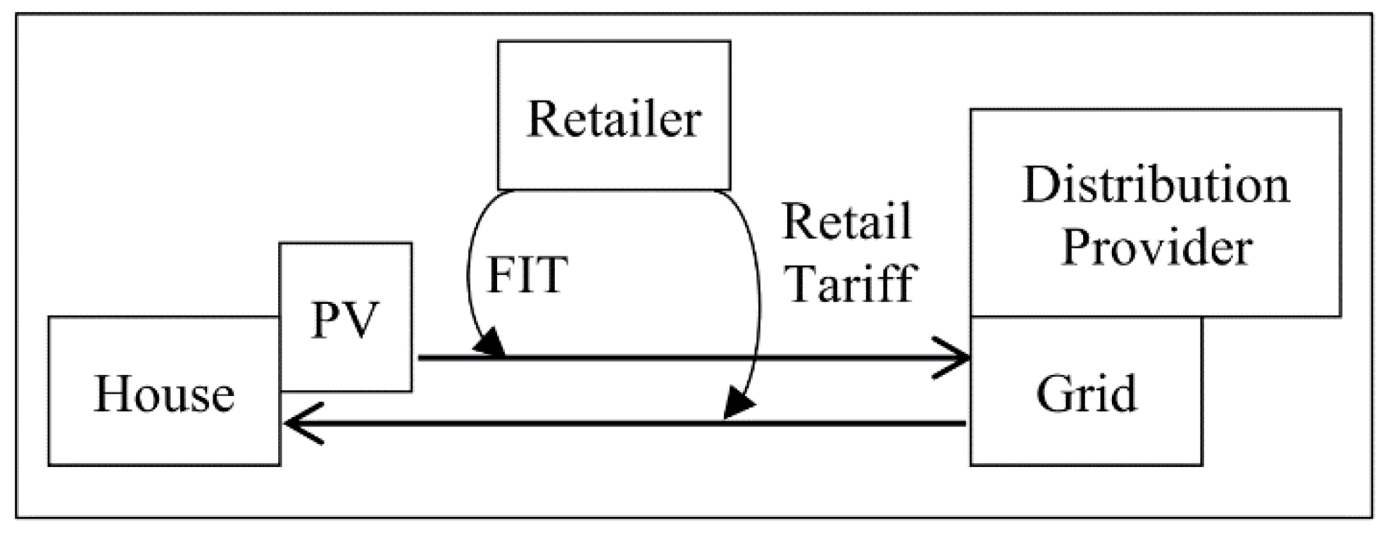
2.1. Feed-in Tariff Model (FiT)

When solar PV first came on the market as a response to increasing the share of electricity production from RES, the investment costs were high because the technology was fairly new. The main objective was to penetrate a high share of RES in the electricity production mix. To do so, the FiT model was implemented.
According to [11], the main idea of the FiT model is to guarantee the investor a form of financial support in the term of investment cost subsidy or an incentive for energy production (for a certain amount of time). As technology improves and installation costs reduce, FiT subsidies or incentives should decrease respectively with time. Values of FiT subsidies and incentives change either by agreement between the EU countries or according to the regulations of each country itself. In general, the values of support tend to and should tend to decline annually. The majority of EU countries have accepted certain models of FiT, where each model is slightly different as they contain elements of subsidies, incentives, and/or remuneration (generally refer to social and environmental costs).
According to data collected in [11], an overview of the FiT models implemented in the various EU and other European countries is shown in Table 1.
As can be seen in Table 1, most of the countries, including Croatia, implemented the FiT model which is based on a form of incentive for energy production (money unit/kWh) over a period agreed by contract.
As stated in [11] and [12], there are two methods for measuring and quantifying the electrical energy of a PV system connected to the grid; the gross metering and net metering method. In the gross metering measurement method, all of the PV production is directly fed to the grid and is subject to FiT, while the consumption of a household is subject to the current retail rates, as shown in Figure 2.
Briefly, all of the PV production is measured by one meter and sold to the grid for FiT rate, while all of the consumption is measured by the second meter and is charged by the retail price.
Using the load profile curve shown in Figure 1a and calculating the PV production curve for a 5.7 kWp PV system for the insolation curve shown in Figure 1b, the energy balance for the FiT model—gross metering method is shown in Figure 3.
As can be seen in Figure 3a, all of the red area under the load profile curve is the consumption of a household and is subject to current retail prices defined by the household’s supplier, while in Figure 3b, all of the green area under the PV profile curve is sent to the grid directly and is subject to the FiT rate defined by the contract between the investor and supplier.
Variants of the FiT model applied in EU and European countries are shown in Table 1. Majority of the countries are using the static model or the flat tariff which means that the elements of financial support like subsidies, incentives, and/or remuneration are determined based on the impact of a PV on an electrical grid. Most of the specified countries apply the flat FiT tariff with a subsidy component in exchange for costs as a consequence of impacting the system due to the stochastic nature of PV. Few other countries applied a high FiT rate to minimize subsidies, such as Denmark, Germany, Spain, and Cyprus [11].
To conclude, there are currently many support models for RES and low carbon technologies (LCT), but the FiT model is shown to be the best model for boosting the LCT development in its early stages, as it guarantees the producers privileged redemption prices for the produced electricity over a certain period as well as it enables them priority access to the power grid according to [13]. When high levels of RES are installed, the FiT model needs to be updated and fitted to a dynamic version of FiT as described in [11] and [12]. Self-supply of domestic households with distributed production from PV is the important direction in which all new installations should be directed and for that purpose, the net-metering model takes its turn.

2.2. Net-Metering Model

The net-metering model is also a PV (RES) market model that is currently gaining huge popularity among the EU countries (and the rest of the world). It has already been implemented in a lot of EU countries and is considered to be the natural transition from the FiT gross metering model. The basic principles are explained and shown in Figure 4, where each country applies specific details regarding the implementation of the model by itself.
While the FiT gross metering model requires two meters to be installed (each in its direction of the flow of electricity), the net-metering model requires only one meter which spins in one direction while the energy is being drawn from the grid (when the consumption is higher than the PV production) and spins in the opposite direction when the energy is being sent to the grid (when the consumption is lower than the PV production).
As opposed to the gross metering measurement method in the FiT model, the net metering measurement method uses the production of PV primarily for household consumption and is subject to retail tariffs, while the excess of produced electrical energy is being sent to the grid and is subject to net-metering, as shown in Figure 4, obtained from [11].
As a part of the net-metering model, there are two types of cost calculations: the net metering method and the net billing method. According to [14], depending on the grid policy, the investor will either get paid for the injected excess electricity or the credits will be saved for the next billing period. In the net metering method, the investor pays the retail price for the net-metered utilized electricity, while the surplus electricity production is getting banked (or temporarily stored) for the upcoming months and that excess is not being sold to the grid. In the net billing method, surplus electricity production is being sold to the grid at a certain rate (i.e., wholesale price of electricity), while the investor pays the retail price for the net-metered utilized electricity. Furthermore, the investor can even integrate his battery storage system, storing the excess electricity to his private storage system (not send it to the grid at that certain moment), and selling it later when the conditions are more favorable, depending on the strategy and algorithm of choice. The electrical energy balance with the grid is shown in Figure 5 and two types of cost calculations in the net-metering model are shown in Figure 6.
Using the load profile curve shown in Figure 1a and calculating the PV production curve for a 5.7 kWp PV system for the insolation curve shown in Figure 1b, the energy balance for the net-metering model is shown in Figure 5.
As can be seen in Figure 5, all of the red area under the load profile curve is the consumption of a household object which has to be drawn from the grid and is subject to current retail prices defined by the household’s supplier. Furthermore, all of the green area under the PV profile curve is produced electrical energy that is sold to the grid directly and is subject to a net-metering rate defined by the contract between the investor and supplier. All of the white area under the blue load profile curve is the amount of electricity that is net-metered, which means that it is produced by the household’s PV system and is all consumed by the household itself directly.
In general, the electricity consumed from the grid is priced higher than electricity exported to the grid. More specifically, electricity imported from the grid is being charged by the retail price, but the electricity exported to the grid is sold at a lower price which means that the credit granted for self-consumers as a remuneration is lower than the retail price. This type of approach makes it more profitable for self-consumers to directly consume the electricity they generate. An increase in self-consumption results in less electricity being drawn from the grid, and thus allows savings at the retail price [15].
A simplified calculation for intuitive understanding has been created to clearly explain the differences between the types of cost calculations in the net-metering model (net metering and net billing methods of calculation). Assuming that the total retail price of the high tariff electricity is 1 (money value/kWh), neglecting the low tariff in this simple calculation and assuming that the redemption price for excess electricity in net billing method is 0.4 (money value/kWh), a total comparative calculation is shown in Figure 6.
As can be seen in Figure 6a, the costs of electricity in the net metering method are active only in January, February, March, and December while being inactive in all the other months of the year. The reason for that is because the electrical energy is stored in the grid and accumulated between April and September and is then spent in October and November. The rest of the difference in December is then paid as a cost because not enough electricity was stored and accumulated into the grid from the previous months. This effect can be best observed by examining the purple curve “monthly cumulative bank” in Figure 6a, where it can be seen that the gradient (slope) of the curve is positive (rising) between March and September (electricity is being stored into the grid) and the gradient is negative (falling) between October and December where previously stored energy is being utilized.
As opposed to that, in the net billing method—Figure 6b, the surplus of energy between April and September is being sold to the grid (by a lower price than retail) and the rest of the months is being charged normally as net-metered utilized energy. Basically, the net metering method could be observed as a calculation method where the surplus is being sold to the grid at full retail price. If it is observed in that way, then it is more financially favorable than the net billing method, where the redemption price is below the retail one. Each country is implementing its version of the net-metering model using the net metering or net billing method. The Croatian model of net-metering is using the net billing method and it will be explained and simulated in the following subheading.
Furthermore, the net-metering model can also be operating under the “virtual” regulations. This type of approach enables electricity generated in one site to be subtracted from the costs for another site and, therefore, more self-consumers can benefit. This is called Virtual net-metering and is currently not widely spread in the EU.
Another very important feature of the net-metering model is that it accelerates the development and installation of smart meters which give consumers access to precise and real-time information regarding the amount of electricity they produce, consume, or export to the grid. Smart meters also tell the price of electricity at which it is charged or bought by the grid. Integrating the artificial intelligence and optimization algorithms with such smart meters could enable the real-time pricing model to be more market responsive and could motivate prosumers to export surplus of the electricity at peak hours when the demand is high and thus gain higher economic value. Consequently, in this case, the prosumers would actively contribute to mitigating grid congestion. Opposite of that, the algorithm would opt to postpone their consumption for after the demand peak, when electricity supply largely meets the demand. Unfortunately, the combinations of the net-metering model and smart metering are not yet widespread practice in the EU [15].
Comparing certain countries gives a good preview of different directions in which the net-metering model was implemented in the EU members. Such a comparison is shown in Table 2 obtained from [15,16], where the countries of Cyprus, Flanders (Belgium), Greece, Italy, and Poland are examined.
According to [15], the Italian net billing system is well established. Their grid operator primarily aims to ensure the stability of the system by charging grid costs, offering remuneration priced lower than retail, and limiting the maximum capacity per contract at 500 kWp.
On the other hand, Flanders (Belgium) has just recently introduced the net billing method as a response to the immoderate expansion of net metering installations. Net metering is therefore expected to function as a demand response model and aims to increase the efficiency and flexibility of the Flemish power system. In addition, due to the 10 kWp limit, the Flemish net billing model is limited for small self-consumers.
Cyprus yet takes a cautious methodology. They have implemented a base framework of the net metering method but with reforms on an annual basis. Basically, when the annual capacity is filled, a new project can enter only in the next year.
Greece is the unique one. Greece introduced net-metering to replace the FiT model. Their regime is quite generous and consists of remuneration at the retail price, long term contracts, billing period every three years where surpluses can be banked and rolled over for 36 months (as opposed to the usual 12 months), the higher limit for maximum capacity per contract, no grid charges, and special provisions for certain islands. In addition, Greece is the first EU country that introduced virtual net metering in 2017. By doing so, the investors have an opportunity to join together and maximize their profit [15].
Poland has developed the “My Electricity” program which aims to increase the availability of prosumer solutions in households (particularly in rural areas). The main objective is to increase the production of electricity from micro-PV systems ranging between 2 and 10 kWp. The program started in August 2019 and until August 2020 the total installed PV capacity was 367.1 MWp, where the average PV installation power was 5.69 kWp [16].

2.3. Net-Metering Model in Croatia

According to [17], the net-metering model in Croatia was established in 2018. Moreover, according to [17], in the territory of the Republic of Croatia, electricity suppliers are obliged to take over surplus electricity from end consumers with self-production that meet the following conditions:
  • Have the status of a privileged (RES) producer of electrical energy.
  • Have the right for permanent connection to the power grid as a simple construction object.
  • The total connection power of all power plants in a single connection point does not exceed 500 kWp.
  • Connection power in one direction (into the grid) does not exceed connection power in the other direction (into the household object).
  • Electrical energy has to be delivered through the same connection point as from which it is bought from the grid.
Furthermore, when calculating electricity consumption costs, as well as fees for the network use and fees for renewable energy sources and high-efficiency cogeneration, the amount of electricity that represents the difference between imported and exported to the grid, electricity in a particular tariff is taken into account. If at the end of the billing period (one month) the amount of electricity exported to the network in a particular tariff is higher than the imported amount, the supplier is obligated to take over the surplus of produced electricity at the price of:
Πht_NM = 0.8 · Πht_electricity
Πlt_NM = 0.8 · Πlt_electricity
where Πht_electricity represents the price of electrical energy during the high tariff (HT) with no extra fees added, Πht_NM represents total redemption price for surplus electrical energy during the high tariff in the net-metering model, Πlt_electricity represents only the price of electrical energy during the low tariff (LT) with no extra fees added, Πnt_NM represents total redemption price for surplus electrical energy during the low tariff in the net-metering model.
In each billing period (one month), the supplier issues an invoice to the end customer of the household category for the difference between the electricity taken from and delivered to the grid at a higher and lower tariff. These differences are the basis for the calculation of the fee for the use of the grid and the fee for renewable energy sources and high-efficiency cogeneration.
If the supplier determines that the investor of the solar PV power plant (in the net-metering model) delivered more electricity to the grid in the previous calendar year than he imported from the grid, the investor shall be considered as a prosumer in the current calendar year. The billing model of a prosumer is defined by the following set of rules:
  • if Eel_import_(i) ≥ Eel_export_(i) ∀ i ∈ [1,12]:
    Πprosumer = 0.9 · Πaverage_electricity
  • if Eel_import_(i) < Eel_export_(i) ∀ i ∈ [1,12]:
    Π p r o s u m e r   =   0.9   ·   Π a v e r a g e _ e l e c t r i c i t y ·   E el _ import _ ( i ) E el _ export _ ( i )     i     [ 1 , 12 ]
    where i represents time in months, Eel_import_(i) represents the total electricity imported from the grid in the ith month, Eel_export_(i) represents the total electricity exported to the grid in the ith month, Πaverage_electricity represents the average price of electricity with no extra fees added (such as grid fees, tax, etc.), and Πprosumer represents the total redemption price for surplus electrical energy in the prosumer model.
Directly from Equation (4), it can be seen why it is not profitable to oversize a PV system in net-metering (if oversized, prosumer model). Namely, oversizing the PV system in the net-metering model concerning the household’s actual annual demand will lead to a switch in the investor’s billing model to the prosumer model. Oversizing the PV system will lead to an increase in the denominator of the fraction Eel_import_(i)/Eel_export_(i) which will lead to a decrease of the whole fraction and, therefore, reduce the redemption price itself, thereby reducing the savings in electricity costs and the NPV (Net Present Value) of the whole project. Therefore, calculating the optimal nominal power of a PV system is mandatory. Unlike it was in the FiT model, it is no longer required for a PV system to be as big as possible, but to satisfy the household’s needs on an annual basis.

3. PV Model and Optimization Algorithm

In this paper, the PV grid-connected systems ranging from 2.1 to 6 kWp according to the net-metering model have been considered. The upper defined PV system range is suitable for most typical average households in Croatia. Furthermore, the PV system is connected to the grid using the central DC-AC inverter and DC power optimizers which are connected in series as shown in Figure 1 in [18]. Using Figure 1 from [18] and adjusting it according to the net-metering model, the schematic representation of a grid-connected PV system has been created and is shown in Figure 7.
The model has been simulated for the cities of Zagreb and Split, where the PV systems are oriented to the south with panels fixed at 35°. According to [10], yearly in-plane insolation for Zagreb is 1513 kWh m 2 and for Split it is 1826 kWh m 2 . PV panels used for simulation are monocrystalline and have an efficiency of 18% with total system losses of 8% on an annual basis. The nominal power of one PV panel is 0.3 kWp and its surface area is 1.6 m2.
The labels, as well as their measurement units, are defined as follows:
  • ΔEannual—yearly difference between imported and exported electrical energy (kWh)
  • EPV—yearly production of electrical energy from PV system (kWh)
  • Econs—yearly consumption of electrical energy of a household (kWh)
  • Econs_ht—yearly consumption of electrical energy of a household during HT (kWh)
  • Econs_lt—yearly consumption of electrical energy of a household during LT (kWh)
  • Eimport_ht_(i)—the amount of imported electricity from the grid during the HT in the ith month (kWh)
  • Eimport_lt_(i)—the amount of imported electricity from the grid during the LT in the ith month (kWh)
  • Eexport_ht_(i)—the amount of exported electricity to the grid during the HT in the ith month (kWh)
  • Eexport_lt_(i)—the amount of exported electricity to the grid during the LT in the ith month (kWh)
  • kcons_ht_(i)—coefficient of HT consumption for the ith month (0–1) given in a vector of 12 months
  • kcons_lt_(i)—coefficient of LT consumption for the ith month (0–1) given in a vector of 12 months
  • PPV—the nominal power of a PV system (kWp) → the variable of decision
  • PPV_p—the nominal power of one PV panel (kWp)
  • PPV_vector—vector of possible PPV for a certain case, with a discrete step of PPV_p
  • PPV_binary—vector of binary values for possible PPV, the same length as PPV_vector
  • APV_p—the surface area of one PV panel (m2)
  • Ireff—reference yearly insolation ( kWh m 2 ) for a panel fixed at 35° and oriented to the south
  • ηPV_p—efficiency of one PV panel (0–1)
  • kloss—coefficient of total PV system losses on annual basis (0–1)
  • kins_(i)—coefficient of insolation (0–1) for the ith month given in a vector of 12 months
  • Econs_var—the amount of variable consumption of electricity on annual basis (kWh)
  • EPV_var—the amount of variable PV production of electricity on annual basis (kWh)
  • ΔEvar—the difference between ΔEannual and total variable electricity (Econs_var + EPV_var) (kWh)
  • ΔEvar_MAX—MAX(ΔEvar), upper limit for a 0.3 kWp PV panel (kWh)
  • Πvar_PV—variable costs of a PV system (PV components, installation costs, and maintenance) (EUR). Installation costs are given in EUR and are converted into HRK using the exchange rate of 7.45.
  • Πfix_PV—fixed costs of a PV system (costs of PV project and bidirectional meter) (EUR)
  • Πtot_PV—total investment costs of a PV system (EUR)
  • i—month (1–12)
  • y—year (1–30)
  • Πht—retail price of electricity during HT( HRK kWh )
  • Πlt—retail price of electricity during LT ( HRK kWh )
  • Πht_ws—wholesale price of electricity during HT ( HRK kWh )
  • Πlt_ws—wholesale price of electricity during LT ( HRK kWh )
  • kΠ_NM—the coefficient for a redemption price of electricity according to the net-metering model ( HRK kWh )
  • tproject—the total lifetime of a PV project (years), assumed to be 30 (years)
  • Πbefore—total electricity costs before the installation of a PV system (HRK) (over a period of tproject)
  • Πafter—total electricity costs after the installation of a PV system (HRK) (over a period of tproject)
  • Πsavings—total electricity savings after the installation of a PV system (HRK) (over a period of tproject)
  • kdiscount—the discount rate used in calculations of a PV project (%)
  • NPV—the net present value of a PV project (HRK)
  • PP—payback period of a PV project (years)
Taking into account Equations (1)–(4), the objective function is set to be a minimization of the yearly difference between exported and imported electrical energy ΔEannual (kWh) with respect to specific constraints. Minimizing the ΔEannual, the optimal nominal power of a PV system is obtained according to the Croatian net-metering model, for which the annual (as well as the total) savings and NPV of the project have been maximized. Uncertainties and variabilities on the side of consumption and PV production have been considered and taken into account by optimization constraints, consequently reducing the risk of downgrading the project’s savings and NPV by oversizing the PV system and thus switching to the prosumer model.
The formulation of the objective function can be expressed as follows (Equation (12) [10]):
MIN [ΔEannual (PPV)] → MIN [Econs − EPV (PPV)]
A detailed version of an objective function can be expressed as follows:
MIN [ i = 1 12 E cons ht · k cons ht ( i ) + i = 1 12 E cons lt · k cons lt ( i ) i = 1 12 P PV P PV _ p · A PV _ p + · η PV _ p · I reff · ( 1 k loss ) · k ins ( i ) ]
where PPV is the decision variable and is set to be determined with the following equality constraints:
Δ E annual = [ i = 1 12 E cons ht · k cons ht ( i ) + i = 1 12 E cons lt · k cons lt ( i ) i = 1 12 P PV P PV _ p · A PV _ p + · η PV _ p · I reff · ( 1 k loss ) · k ins ( i ) ]
E cons = i = 1 12 E cons ht · k cons ht ( i ) + i = 1 12 E cons lt · k cons lt ( i )
E PV = i = 1 12 P PV P PV _ p · A PV _ p + · η PV _ p · I reff · ( 1 k loss ) · k ins ( i )
kcons_ht * = [0.0720, 0.0536, 0.0709, 0.0617, 0.0910, 0.0777, 0.0968, 0.0978, 0.0854, 0.1038, 0.0886, 0.1007]
kcons_lt * = [0.0807, 0.0667, 0.0733, 0.0527, 0.0748, 0.0645, 0.0865, 0.1013, 0.0898, 0.1148, 0.0700, 0.1249]
kins = [0.0423, 0.0475, 0.0819, 0.104, 0.1132, 0.119, 0.1272, 0.1208, 0.0936, 0.0716, 0.043, 0.0359]
PPV_p = 0.3
APV_p = 1.6
ηPV_p = 0.18
kloss = 0.08
I reff = { if     Zagreb :   1513 elif   Split :   1826
Econs_var = [−0.05 · (Econs), 0.05 · (Econs)]
EPV_var = [−78.07·Ppv, 78.07·Ppv]
ΔEvar = ΔEannual − (Econs_var + EPV_var)
ΔEvar_MAX = Ireff · APV_p · ηPV_p · (1 − kloss)
PPV_vector = [2.1, …, 6] with a step of PPV_p
P PV _ binary { 0 , 1 } 14
i = 1 14 P PV binary ( i ) = 1
PPV = i = 1 14 P PV binary ( i ) · P PV vector ( i )
Eimport _ ht = i = 1 12 { if     E cons ht ( i ) E PV ht ( i )   0   :   E cons ht ( i ) E PV ht ( i ) else :     0
Eimport _ lt = i = 1 12 { if     E cons lt ( i ) E PV lt ( i )   0   :   E cons lt ( i ) E PV lt ( i ) else :     0
Eexport _ ht = i = 1 12 { if     E cons ht ( i ) E PV ht ( i ) <   0   :   abs ( E cons ht ( i ) E PV ht ( i ) ) else :     0
Eexport _ lt = i = 1 12 { if     E cons lt ( i ) E PV lt ( i ) <   0   :   abs ( E cons lt ( i ) E PV lt ( i ) ) else :     0
and with the following inequality constraints:
ΔEannua ≥ 0
ΔEannual ≥ Econs_var + EPV_var
ΔEvar_MAX ≥ ΔEvar
*—Obtained from research associated with Croatian electrical energy suppliers.
Examining the expressions above, which are describing the optimization algorithm, it can be seen that the main inequality constraint is Equation (30) for the net-metering (net billing) model to be viable and not to activate the prosumer model.
Furthermore, the technical constraint of a PV system exists because the possible PV nominal power can only be a multiple of PPV_p as the nominal power of one PV panel is 0.3 kWp. Hence, this type of optimization problem is a form of discrete optimization which is solved by a specific type of approach. A vector of binary variables, same length as all possible PV powers, is created, whose sum is equal to one, as stated in Equation (24). In this way, only one value can take on the value of one, while all of the other values are zero. Briefly, only one power in the entire interval [2.1, …, 6] can take on a certain value (which is set to be the optimal power), while all of the other possible powers are zero when Equation (25) is implemented. Namely, the Gurobi solver detects expression in Equation (25) as a quadratic constraint, thus the problem becomes a quadratically constrained optimization problem. Any problem simulated within the boundaries stated above, the Gurobi solver can solve in 0.03 s with a thread count of 1 (of 4 available processors) using a Intel® Core™ i7-6600 CPU @ 2.60 GHz (4 CPUs), ~2.8 GHz and 8 GB of RAM.
Variable investment costs (system components, installation, and maintenance) for the above-described PV system can be, regarding the interval from 2.1 to 6 kWp, expressed as the following linear function:
Πvar_PV (PPV) = 860.82 · PPV + 575.88 #
while fixed costs consist of the cost for the PV project and the cost of bidirectional meter which amount to:
Πfix_PV = (270 + 400) = 670 #
#—Obtained from research associated with Croatian electrical energy and PV suppliers.
The total investment costs of a PV system can be calculated according to the following equation:
Πtot_PV = Πtot_PV + Πfix_PV
To calculate the total electricity costs before and after the installation of the PV system, prices, and fees of HT and LT electricity are given in Table 3.
The total electricity costs before the installation of the PV system are calculated as follows:
Π before = y = 1 30 ( i = 1 12 E cons _ ht ( y ) ( i ) · Π ht + i = 1 12 E cons _ lt ( y ) ( i ) · Π lt )
The total electricity costs after the installation of the PV system are calculated as follows:
Π after = i = 1 30 ( i = 1 12 E import _ ht ( y ) ( i ) · Π ht + i = 1 12 E import _ lt ( y ) ( i ) · Π lt i = 1 12 E import _ ht ( y ) ( i ) · Π ht ws · k Π NM i = 1 12 E import _ lt ( y ) ( i ) · Π lt ws · k Π NM )
The total electricity savings can be then calculated as:
Πsavings = Πbefore − Πafter
The authors of [19] used a stochastic approach with Monte Carlo simulation and calculated discount rates for Korean PV investment projects which amounted to 4.5%, 5.5%, and 7.5% for min, mean, and max values according to the triangular distribution. The authors also stated that the current rate amounts to 5.5%, but requires a reduction of 1% in the future, so the rate used in this simulation amounts to:
kdiscount = 0.045
An expression used for calculating the NPV of a project is obtained from [20]:
NPV = y = 1 30 Π savings ( y ) ( 1 + k discount ) y Π tot _ PV
where the total savings during the year y ( Π savings ( y ) ) are considered to be the net cash inflow and the project is considered to be valid if the NPV is greater than zero.
Furthermore, the expression for calculating payback period (PP) is also obtained from [20]:
PP = Π tot PV y = 1 30 Π savings ( y ) ( 1 + k discount ) y
The simulation results are shown and discussed in the following chapter.

4. Results

This section contains numerical solutions and results of the previously stated mathematical model for the presented optimization problem. Furthermore, the solution for the optimization problem is not expressed as a single value, but rather as a vector of solutions depending on the total annual electricity consumption in HT.
For this purpose, the main optimization model has been nested inside of a loop which iterates annual HT electricity production in a range from 2100 kWh up to 6000 kWh with a step of 1 kWh, so that the vector of optimal nominal powers can be obtained. In addition, the model has been simulated for the locations of Zagreb and Split to conduct a comparative analysis.
Furthermore, the algorithm was simulated for multiple scenarios of variability in electricity production and consumption. Examining the drivers of change in annual average energy consumption per household, obtained from [21], the annual variability of electricity consumption is set to vary from −5% to +5% of the total annual electricity consumption, as previously expressed in Equation (18).
According to [10] and with regards to input parameters used in the PV model (i.e., geographic location, slope angle, azimuth angle, the efficiency of PV, as well as total losses of a system), the variability of the annual electricity PV system production is set to vary from −78.07 kWh kWp for Zagreb (or −70.53 kWh kWp for Split) to +78.07 kWh kWp for Zagreb (or +70.53 kWh kWp for Split). For the simplicity of use and due to the small difference between annual PV production variability between Zagreb and Split, parameters used in the loop simulation are those for the geographic location of Zagreb.

4.1. Optimal PV Power Simulations

Results obtained from the simulation showing the optimal nominal powers with respect to the change in annual HT electricity production are shown in Figure 8.
Namely, the first main observation which can be seen in all six subfigures in Figure 8 is that the optimal nominal powers for all types of variability for Split are slightly lower than those for Zagreb. The main reason for this is the fact that the insolation for Split is higher than the insolation in Zagreb, so that the same nominal power PV system in Split will annually produce more electricity than the PV system in Zagreb. In addition, the shapes of all curves in Figure 8 are in discrete distribution because the step of change in the PV system’s power is 0.3 kWp (rated power of 1 PV panel).
Figure 8a,b represents results for scenarios in the variability of PV production for Zagreb and Split. As can be seen, an increase in annual PV production results in a decrease of the needed optimal nominal power. Consequently, a decrease in annual PV production increases the needed optimal nominal power. The PV production and optimal PV power are inversely proportional.
Furthermore, examining the results shown in Figure 8c,d, the opposite effect can be seen. The increase in annual electricity consumption increases the needed optimal nominal power. Vice versa, the decrease in annual PV production results in a decrease of the needed optimal nominal power. The electricity consumption and optimal PV power are proportional.
Lastly, examining Figure 8e,f, boundary (marginal) scenarios can be observed. As can be concluded from the previous statements regarding the proportionality between parameters, SCENARIO 1 represents the upper boundary scenario with a simultaneous increase of the annual consumption by 5% and a decrease of PV production by 78.07 kWh kW . Opposite of that, SCENARIO 2 represents the lower boundary scenario with a simultaneous decrease of the annual consumption by 5% and an increase of PV production by 78.07 kWh kW . Interesting to observe is that these boundary scenarios disperse the curves of optimal powers in a wider manner than in previous cases, which is logical and natural.
In addition, two sub-scenarios (a sub-scenario is considered to be one specific solution from the vector of solutions which is referred to as scenario) can be seen on the graphs; the first one is on subfigure (e) on the curve SCENARIO 1 in the area of maximum values of optimal powers, 6 kWp. As the consumption increases and the production decreases, the optimal nominal power should increase in a discrete step over the value of 6 kWp, but the optimization algorithm keeps the values locked up at 6 kWp, because of the constraint PPV_vector expressed in Equation (22).
Similarly, the second sub-scenario occurs in the subfigure (f) on the curve SCENARIO 2 in the area of minimum values of optimal powers, 2.1 kWp. As the consumption decreases and the production increases, the optimal nominal power should decrease in the discrete step below the value of 2.1 kWp, but the optimization algorithm keeps the values locked up at 2.1 kWp, because of the constraint PPV_vector also expressed in Equation (22).

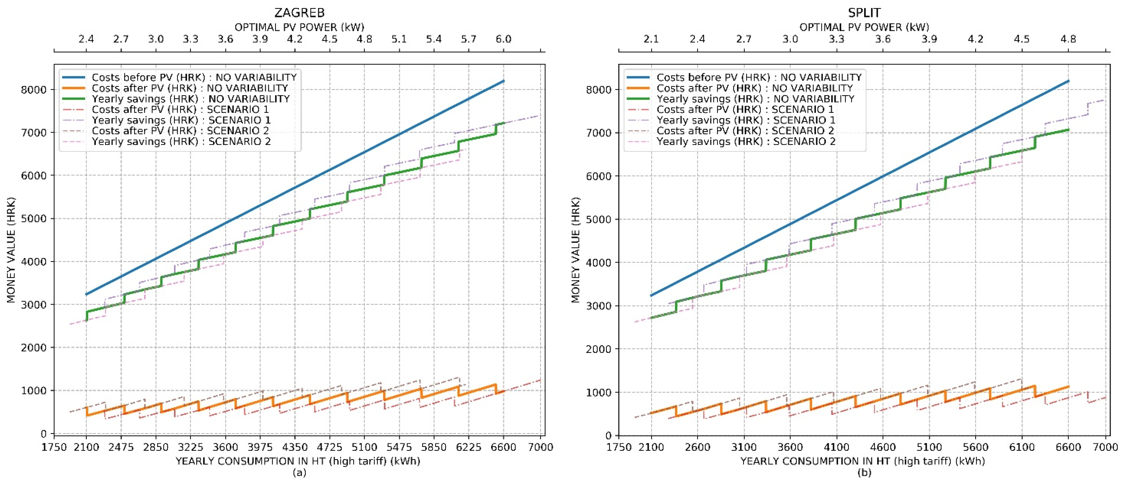
4.2. Energy Balance and Financial Simulations

To examine the optimization algorithm results in closer detail, the electricity balance simulation results between household and grid are shown in Figure 9.
As can be observed from the green curve “Difference in energy” in Figure 9, when the optimization algorithm sets the optimal nominal power to a certain optimal value, it stays in that discrete value range for as long as the difference in electricity between import and export enables it to stay in that range. For the location of Zagreb, this value is around 400 kWh, while for Split this range of maximum difference in electricity is around 500 kWh, which corresponds to the maximum production of one PV panel (in ideal conditions).
Observing the curves “Energy from the grid” and “Energy to the grid” it can be seen that at a certain point both curves start from the same value (where the difference is zero) and they start spreading apart until the maximum value of the difference in electricity is reached. At this point, the optimization algorithm increases the optimal nominal power by 0.3 kWp and the difference in electricity again becomes zero. As the two mentioned curves start spreading apart, it can be seen that the “Energy from the grid” curve starts to increase, while the “Energy to the grid” curve starts to decrease. The reason for that is the fact that the total electricity consumption in HT increases, but the optimal nominal power in that interval stays the same until the boundary sub-scenario is reached at which point the algorithm increases the optimal nominal power, causing the total difference in electricity to become zero again. The following figure shows the advantage of using renewable energy sources (in this case PV systems), whose costs of fuel (sunlight) are zero, making the costs of electricity drop significantly.
Figure 10 represents the advantages of using RES more closely. Namely, the difference in annual costs of electricity before and after the installation of a PV system (annual savings) is significant. Comparing Zagreb and Split for the same annual consumption scenario, without variability, it can be concluded that households in Zagreb have slightly lower costs of electricity and slightly higher savings of electricity on annual basis, due to the higher optimal nominal power of a PV system (which then produces and exports more electricity), than Split.
In addition, a second x-axis is added in Figure 10, Figure 11 and Figure 12. Namely, this upper x-axis contains discrete values of optimal nominal powers for each HT electricity consumption interval respectively. Values shown in the mentioned x-axis are parameterized for the “NO VARIABILITY” curves (solid lines), which are considered to be the base scenarios.
Furthermore, in Figure 11 it can be observed that PP is lower for a household in Split than in Zagreb (again for the same annual consumption scenario).
Because of the higher optimal nominal power of a PV system (which then produces and exports more electricity), Zagreb has slightly lower costs of electricity and slightly higher savings of electricity on annual basis than Split. Consequently, Zagreb has higher investment costs and so the PP values are higher. A household with the same annual electricity consumption for Split has a lower optimal nominal power than Zagreb, so the investment costs are lower as well, hence the PP is lower.
Furthermore, the NPV is also considered as one of the main criteria for the financial evaluation of the projects, so it has been included in this paper. Namely, the NPV is calculated for every scenario and sub-scenario in this simulation and the results are shown in Figure 12.
Examining the results for NPV from Figure 12 it can be seen that the NPV of a PV project for Split is higher than for Zagreb, considering the same annual consumption scenario. The reason for that is the same as for the PP. A household with the same annual electricity consumption for Split has a lower optimal nominal power than Zagreb, so the investment costs and PP are lower as well, hence the NPV is higher.

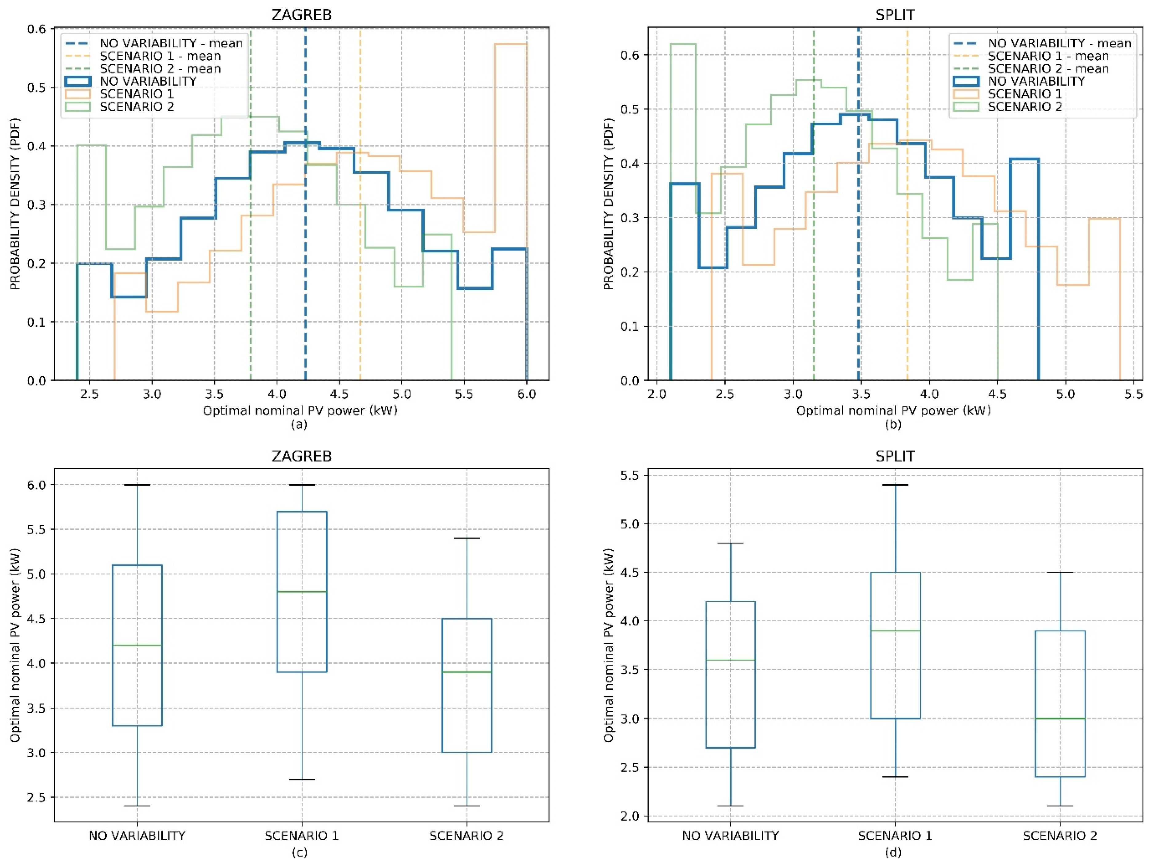
4.3. Statistical Analysis of the Obtained Results

Lastly, by statistically processing the vector of calculated optimal nominal powers for all three scenarios, Figure 13 is created.
Figure 13 represents the statistical view of the results presented in Figure 8 and is convenient for the comparison analysis between Zagreb and Split. Namely, on subfigures (a) and (b) the Gaussian distribution is shown. The distribution has been created using Numpy’s random.normal method (with mean and standard deviation values obtained from the results presented in Figure 8) and using Numpy’s clip method for limiting the Gaussian distribution in min and max values of optimal nominal powers. As mentioned earlier, the mean values of optimal powers are lower for Split than for Zagreb. In addition, electricity variability defined as Scenario 1 shifts distribution to a higher nominal power area (to the right), while Scenario 2 shifts distribution to a lower nominal power area (to the left). In subfigures (c) and (d) a boxplot diagram is presented with interquartile range. Similarly, as with the mean values, the median values for Split are lower than those for Zagreb, due to higher insolation and PV production in Split.

4.4. Discussion of Results

Considering all the results shown and analyzed above, it is concluded that Split has a positive advantage over Zagreb when installing a grid-connected PV system in a net-metering model. The advantage occurs due to the already mentioned higher insolation and PV production in Split.
Namely, Split is considered to be the representative city for the Mediterranean region of Croatia as it has much more insolation than Zagreb, while Zagreb is considered to be the representative city for the continental region of Croatia. For the same annual HT consumption, optimal PV power in Split is lower than in Zagreb. This is making PV projects in Split slightly more profitable than those in Zagreb. Furthermore, as optimal PV powers in Zagreb are higher than in Split, PV systems in Zagreb produce and export more electricity so that the costs of electricity are lower and the savings on electricity are higher. However, since Zagreb has higher optimal PV powers, so that the investment costs are also higher and the PP values result in being higher than in Split. The PP values obtained from the simulation range between 6.7 and 13.3 years for Zagreb and between 5.7 and 11.5 years in Split depend on the discount rate, PV production, and household consumption. Furthermore, all the PV projects for Zagreb and Split have PP values less than 10 years, if observed with no discount rate (discount rate = 0%). Considering all the results simulated regarding the financial evaluations of the PV projects, it can be concluded that it is highly profitable to install micro-PV household systems according to the Croatian net-metering model. The net-metering model enables household consumers to become active prosumers and participate in their electricity cost reduction, where the power grid acts as electricity storage for the surplus. However, it is important to determine the optimal PV power for each project individually, as each project is described by its own set of parameters. Oversizing the PV system in the net-metering model will lead to a switch in the investor’s billing model to the prosumer model which will then decrease the project’s NPV and increase its PP value.

5. Conclusions

The European Union is determined to be the global leader in the fight against climate change. The EU aims to lead by example through the implementation of key points in the European Green Deal.
This paper solves a quadratically constrained optimization problem for determining the optimal nominal power of a grid-connected PV household system according to the Croatian net-metering model. Results presented in this paper show that it is highly profitable to install micro-PV household systems in Croatia in the net-metering model as they reduce the electricity costs significantly. Most of the simulated PV projects have a PP value lower than 10 years (except the ones with higher discount rates) and considering the fact that PV systems have a lifetime of 30 years, it makes them distinctly profitable. However, oversizing the PV system with regards to the annual electricity consumption of a household results in an increase of the surplus of electricity exported to a grid on a higher level than imported electricity. This makes the calculation of the costs switch from the net-metering model to the prosumer model, as stated in Croatian law [13], and thus decreasing the profitability of a PV project by increasing the PP and decreasing the NPV. The results of the comparative analysis between Zagreb and Split for multiple scenarios of variability in consumption and production are presented. Due to higher insolation and PV production, Split has a slight advantage as optimal nominal powers are lower than for Zagreb, so that the investment costs drop as well as the PP of the project, while the NPV increases. Nevertheless, PV projects for both locations of Zagreb and Split are highly profitable due to the low marginal costs of production from a PV system. From the grid’s perspective, the optimal nominal power of a PV system reduces unnecessary surpluses of electricity into the grid and thus reducing the additional costs of operating the grid and increasing its flexibility.
In future research, this paper can be expanded by analyzing the integration of battery storage systems, heat pumps, and electric vehicles with two-way charging dynamics. Furthermore, using deep learning algorithms for predicting the electricity production from PV and household consumption, as well as integrating it with the previously mentioned energy systems will be considered in future research.

Author Contributions

Conceptualization and methodology, L.B., G.G. and M.D.; software, validation, formal analysis and visualization, L.B.; supervision, resources and funding acquisition, M.D.; writing—original draft preparation, L.B.; writing—review and editing, G.G. and M.D. All authors have read and agreed to the published version of the manuscript.

Funding

This paper is partly based on research developed through the project “Integrated solution for asset management and support of investment processes of design, planning, and implementation of renewable energy sources construction” supported by the European Union within the European Regional Development Fund (KK.01.2.1.02.0146). This paper is partly based on research developed through the project “METAR—A meter to a Better Climate—Network for Education, Transition, Adaptation and Development” supported by the European Union within the European Social Fund (UP.04.2.1.06.0029).

Conflicts of Interest

The authors declare no conflict of interest.

References

  1. IEA-ETSAP; IRENA. Renewable Energy Integration in Power Grid: Technology Brief; IRENA: Abu Dhabi, UAE, 2015. [Google Scholar]
  2. Twidell, J.; Weir, T. Renewable Energy Resources, 3rd ed.; Routledge: London, UK, 2015. [Google Scholar]
  3. Kryzia, D.; Olczak, P.; Wrona, J.; Kopacz, M.; Kryzia, K.; Galica, D. Dampening Variations in Wind Power Generation Through Geographical Diversification. IOP Conf. Ser. Earth Environ. Sci. 2019, 214, 012038. [Google Scholar] [CrossRef]
  4. Szablicki, M.; Rzepka, P.; Sołtysik, M.; Czapaj, R. The idea of non-restricted use of LV networks by electricity consumers, producers, and prosumers. In Proceedings of the 14th International Scientific Conference “Forecasting in Electric Power Engineering” (PE 2018), Podlesice, Poland, 26–28 September 2018; p. 84. [Google Scholar]
  5. Kuchmacz, J.; Mika, L. Description of development of prosumer energy sector in Poland. Polityka Energetyczna Energ. Policy J. 2018, 21, 5–20. [Google Scholar] [CrossRef]
  6. Wang, H.; Lei, Z.; Zhang, X.; Zhou, B.; Peng, J. A review of deep learning for renewable energy forecasting. Energ. Convers. Manag. 2019, 198, 111799. [Google Scholar] [CrossRef]
  7. Bayindir, R.; Demirbaş, Ş.; Irmak, E.; Cetinkaya, U.; Ova, A.; Yeşil, M. Effects of renewable energy sources on the power system. In Proceedings of the 2016 IEEE International Power Electronics and Motion Control Conference (PEMC), Varna, Bulgaria, 18–23 September 2016; pp. 388–393. [Google Scholar]
  8. Saqib, N.; Haque, K.F.; Zabin, R.; Preonto, S.N. Analysis of Grid Integrated PV System as Home RES with Net Metering Scheme. In Proceedings of the International Conference on Robotics, Electrical and Signal Processing Techniques (ICREST), Dhaka, Bangladesh, 10–12 January 2019; pp. 395–399. [Google Scholar]
  9. Soria, M.; Vásquez, P. Deterministic and stochastic optimization-based decision-making approaches for effectively coping with residential photovoltaic micro-systems sizing problem under net-metering schemes. In Proceedings of the IEEE Fourth Ecuador Technical Chapters Meeting (ETCM), Guayaquil, Ecuador, 13–15 November 2019; pp. 1–6. [Google Scholar]
  10. PVGIS. Available online: https://re.jrc.ec.europa.eu/pvg_tools/en/#PVP (accessed on 11 December 2020).
  11. Prahastono, I.; Sinisuka, N.I.; Nurdin, M.; Nugraha, H. A Review of Feed-In Tariff Model (FIT) for Photovoltaic (PV). In Proceedings of the 2nd International Conference on High Voltage Engineering and Power Systems, Denpasar, Indonesia, 2–5 October 2019; pp. 76–79. [Google Scholar]
  12. Olivia, S.; McGill, I. Dynamic Model Approach To Assess Feed In Tariffs For Residential Pv Systems. In Proceedings of the International Association of Energy Economics (IAEE) Conference, Daegu, Korea, 16–20 June 2013. [Google Scholar]
  13. Punda, L.; Capuder, T.; Pandžić, H.; Delimar, M. Integration of renewable energy sources in southeast Europe: A review of incentive mechanisms and feasibility of investments. Renew. Sustain. Energ. Rev. 2017, 71, 77–88. [Google Scholar] [CrossRef]
  14. Alasadi, S.; Abdullah, M.P. Comparative Analysis between Net and Gross Metering for Residential PV System. In Proceedings of the IEEE 7th International Conference on Power and Energy (PECon), Kuala Lumpur, Malaysia, 3–4 December 2018; pp. 434–439. [Google Scholar]
  15. Iliopoulos, T.G.; Fermeglia, M.; Vanheusden, B. The EU’s 2030 Climate and Energy Policy Framework: How net metering slips through its net. Rev. Eur. Comp. Int. Environ. Law 2020, 29, 245–256. [Google Scholar] [CrossRef]
  16. Olczak, P.; Kryzia, D.; Matuszewska, D.; Kuta, M. “My Electricity” Program Effectiveness Supporting the Development of PV Installation in Poland. Energies 2021, 14, 231. [Google Scholar] [CrossRef]
  17. NARODNE NOVINE. Available online: https://narodne-novine.nn.hr/clanci/sluzbeni/2018_12_111_2151.html (accessed on 15 December 2020).
  18. Zhang, X.; Chen, M.; Fu, Y.; Li, Y. A Step-Down Partial Power Optimizer Structure for Photovoltaic Series-Connected Power Optimizer System. In Proceedings of the IEEE International Power Electronics and Application Conference and Exposition (PEAC), Shenzhen, China, 4–7 November 2018; pp. 1–4. [Google Scholar]
  19. Lee, C.-Y.; Ahn, J. Stochastic Modeling of the Levelized Cost of Electricity for Solar PV. Energies 2020, 13, 3017. [Google Scholar] [CrossRef]
  20. Aleksiejuk-Gawron, J.; Milčiuvienė, S.; Kiršienė, J.; Doheijo, E.; Garzon, D.; Urbonas, R.; Milčius, D. Net-Metering Compared to Battery-Based Electricity Storage in a Single-Case PV Application Study Considering the Lithuanian Context. Energies 2020, 13, 2286. [Google Scholar] [CrossRef]
  21. EEA. Available online: https://www.eea.europa.eu/data-and-maps/daviz/drivers-of-the-change-in-4#tab-chart_2 (accessed on 19 January 2021).
Figure 1. (a) Statistically processed samples of load consumption. (b) Profile curve of PV insolation.
Energies 14 01746 g001
Figure 2. Gross metering measurement method [11].
Energies 14 01746 g002
Figure 3. Electrical energy balance between household and power grid according to the FiT model. (a) Electricity from the grid. (b) Electricity to the grid.
Energies 14 01746 g003
Figure 4. Net metering measurement method.
Energies 14 01746 g004
Figure 5. Electrical energy balance between household and power grid according to the net-metering model.
Energies 14 01746 g005
Figure 6. (a) Net metering type of cost calculation. (b) Net billing type of cost calculation.
Energies 14 01746 g006
Figure 7. Schematic representation of a grid-connected PV system in a net-metering model.
Energies 14 01746 g007
Figure 8. The optimal nominal power of a PV system: (a) Variability in PV production for Zagreb. (b) Variability in PV production for Split. (c) Variability in total consumption for Zagreb. (d) Variability in total consumption for Split. (e) Boundary scenarios of variability for Zagreb. (f) Boundary scenarios of variability for Split.
Energies 14 01746 g008
Figure 9. Simulation results for electricity balance between household and grid scenario without variability: (a) Simulation results for Zagreb. (b) Simulation results for Split.
Energies 14 01746 g009
Figure 10. Simulation results for electricity costs and savings before and after the installation of the PV system. (a) Simulation results for Zagreb. (b) Simulation results for Split.
Energies 14 01746 g010
Figure 11. Simulation results of the payback period for a PV system project with discount rates of 0% and 4.5%. (a) Simulation results for Zagreb. (b) Simulation results for Split.
Energies 14 01746 g011
Figure 12. Simulation results of the net present value (NPV) for a PV system project with discount rates of 0% and 4.5%. (a) Simulation results for Zagreb. (b) Simulation results for Split.
Energies 14 01746 g012
Figure 13. (a) Gaussian distribution of optimal powers with mean values for Zagreb. (b) Gaussian distribution of optimal powers with mean values for Split. (c) Boxplot diagram of optimal powers with interquartile range for Zagreb. (d) Boxplot diagram of optimal powers with interquartile range for Split.
Energies 14 01746 g013
Table 1. Variants of the FiT model implemented in certain EU and other European countries.
CountriesComponents of FiTRemarks
NetherlandsInvestment cost subsidy-
Austria, Belgium, and SwedenInvestment cost subsidy.
Incentive for energy production.
The amount of incentives depends on the current regulations in certain countries respectively.
BIH, Bulgaria, Cyprus, Czech Republic, Estonia, Hungary, England, Italy, Germany, Croatia, Latvia, Lithuania, Luxembourg, Macedonia, Malta, Montenegro, France, Portugal, Romania, Serbia, Slovakia, Slovenia, Spain, Switzerland, Ukraine, GreeceIncentive for energy production over a certain period.The amount of incentives depends on the type and capacity of PV, location, and the regulations that apply in each sector or part of a certain country respectively.
Table 2. Comparison of net-metering models in certain EU countries [15,16].
EU CountryTypeContracts DurationGrid ChargesAggregated Installed Capacity LimitConsumers InvolvedTechnologies
CyprusNet metering,
Net billing
10 or 15 yearsResidential and low-voltage non-residential (up to 10 kWp each)Solar PV for net metering, all RES for net billing
Flanders (Belgium) Net metering,
Net billing
Up to 10 kWpAll renewable electricity
Greece Net metering,
Virtual net metering
25 yearsResidential and non-residential (up to 1 MW)All renewable electricity
ItalyNet billing1 year (automatic renewal)Residential and non-residential (up to 500 kWp)All renewable electricity
PolandNet billing1 yearResidential and non-residential (up to 50 kWp)Solar PV
Table 3. Input values for the calculation of electricity price.
Elements of PriceHT (High Tariff)LT (Low Tariff)
Wholesale price (HRK/kWh)0.490.24
Grid fee (HRK/kWh)0.350.17
RES fee (HRK/kWh)0.1050.105
Solidarity fee (HRK/kWh)0.030.03
Electricity TAX0.130.13
Total retail price (HRK/kWh)1.100.62
Publisher’s Note: MDPI stays neutral with regard to jurisdictional claims in published maps and institutional affiliations.

