Design Selection and Geometry in OWC Wave Energy Converters for Performance

Abstract

Although oscillating water column (OWC) wave energy converters are arguably one of the most studied technologies, it is not clear which chamber geometry, among all of the available alternatives, would provide the best performance at a site of interest. In this work, a numerical model based on the Navier-Stokes equations for two compressible fluids, using a volume-of-fluid interface-capturing approach, is implemented to determine the best performing OWC geometry in a case study off the Port of Vigo (NW Spain). Four general shapes of OWC are analyzed: classic, stepped-bottom, U-shaped and L-shaped, and geometrical variants are investigated. In total, 18 chamber geometries are studied, considering the same turbine geometry in all of them. It was found that the U-shaped and L-shaped designs are the most easily tuned to resonate at a period of interest. Of these two, the L-shaped performs better. The best performance is achieved for an L-shaped OWC design with a shallow entrance, a high horizontal chamber duct and a wide vertical duct, for which a maximum capture-width ratio of 71.6% was achieved.

1. Introduction

Oscillating water column (OWC) devices are one of the most studied wave energy conversion technologies so far [1]. An OWC consist of an empty chamber opened to the sea below the surface, and an air turbine. Wave action causes the oscillation of the water column inside the chamber, alternately compressing and decompressing the air in the upper part of the chamber. The pressure difference created between the interior of the chamber and the atmosphere forces the air to move in and out of the chamber, driving the turbine in the process. Due to the bidirectional characteristics of the flow, a special solution is required to harvest the greatest amount of available pneumatic energy per cycle. The most common solution are the self-rectifying air turbines [2], although there are other alternatives as the vented OWCs, a novel design that, by using passive rectifying air flow valves in the chamber, works with unidirectional turbines [3]. Among self-rectifying air turbines, Wells (reaction) turbines [4] and impulse turbines, both axial [5], radial [6], or the novel biradial [7], are at the forefront of the developments.

However, not only the turbine design is important in order to maximize the performance of an OWC device, the chamber geometry is also an essential aspect. The chamber must be designed to ensure near-resonant conditions with the incident waves and, at the same time, to avoid energy losses. In this context, the geometry of OWC converters has been widely analyzed in recent literature. A special design of OWC, equipped with an extra front wall that causes the OWC chamber to be connected to the sea through a vertical duct, increasing the natural oscillation frequency of the water column was proposed in [8]. As a result of this configuration this device is known as U-shaped OWC. Rezanejad et al. [9] proposed a new configuration of the OWC by locating a step in front of the chamber. The step adds a new resonant mechanism that takes place when the water volume above the step acts similarly to a rigid piston with its natural frequency of oscillation being close to the frequency of the incident wave. There exist also L‑shaped OWC geometries in which a duct oriented in the direction of wave propagation is used to increase the resonant frequency of the system [10,11]. This concept was also used in the OWC module of the hybrid wave energy converter proposed in [12] that merges an OWC and an overtopping device. When the OWC is designed to be isolated, the cylindrical shape is one of the most common alternatives given that this solution is not affected by wave direction [13]. It was proposed both for nearshore devices [14,15] as well as for hybrid wind-wave applications [16]. Hybrid wave farms combining OWC WECs with other wave energy conversion technologies have also been investigated [17,18]. In addition, many studies investigate the performance improvements that specific geometric modifications introduce in an OWC converter, e.g., variations in the slope of the front and rear walls of the chamber [19], or the effects of the length and the opening angle of harbor walls (a pair of sidewalls in front of the device) [20]. Finally, OWC technology lends itself to the installation of multiple chambers, integrated e.g., in floating platforms or deployed along the coast as part of a structure [21,22]. In all the mentioned cases, both on the offshore and the nearshore OWC devices, the optimization of the chamber geometry has to be carried out taking into account the wave climate at the locations of interest, being necessary to characterize the wave conditions that provide the bulk of energy (e.g., [23,24,25]).

Despite the efforts of the last few years to obtain optimized OWC geometries, it is not straightforward to select a design for a new plant at a site of interest. In this work, a bidimensional numerical model is implemented to determine the best performing OWC design for a given site. The numerical model is based on the RANS-VOF numerical wave flume implemented and validated in previous works [26,27] but improved in order to take into account the spring-like effect of the air compressibility, a factor that meaningfully affects the performance of an OWC converter [28]. The restrictions imposed on the OWC designs in this study are: (i) the design must lend itself to integration into a coastal structure; and (ii) its construction should be easy (avoiding intricate geometries) for containing costs. In this way, the solution achieved would be applicable to a wide range of ports. Four main general shapes of OWC are analyzed: classic, stepped-bottom, U-shaped and L-shaped; and for each of them different geometrical modifications are considered. In total, 18 geometries are studied. The work is illustrated through a case study in the surroundings of the Port of Vigo (NW Spain).

2. Materials and Methods

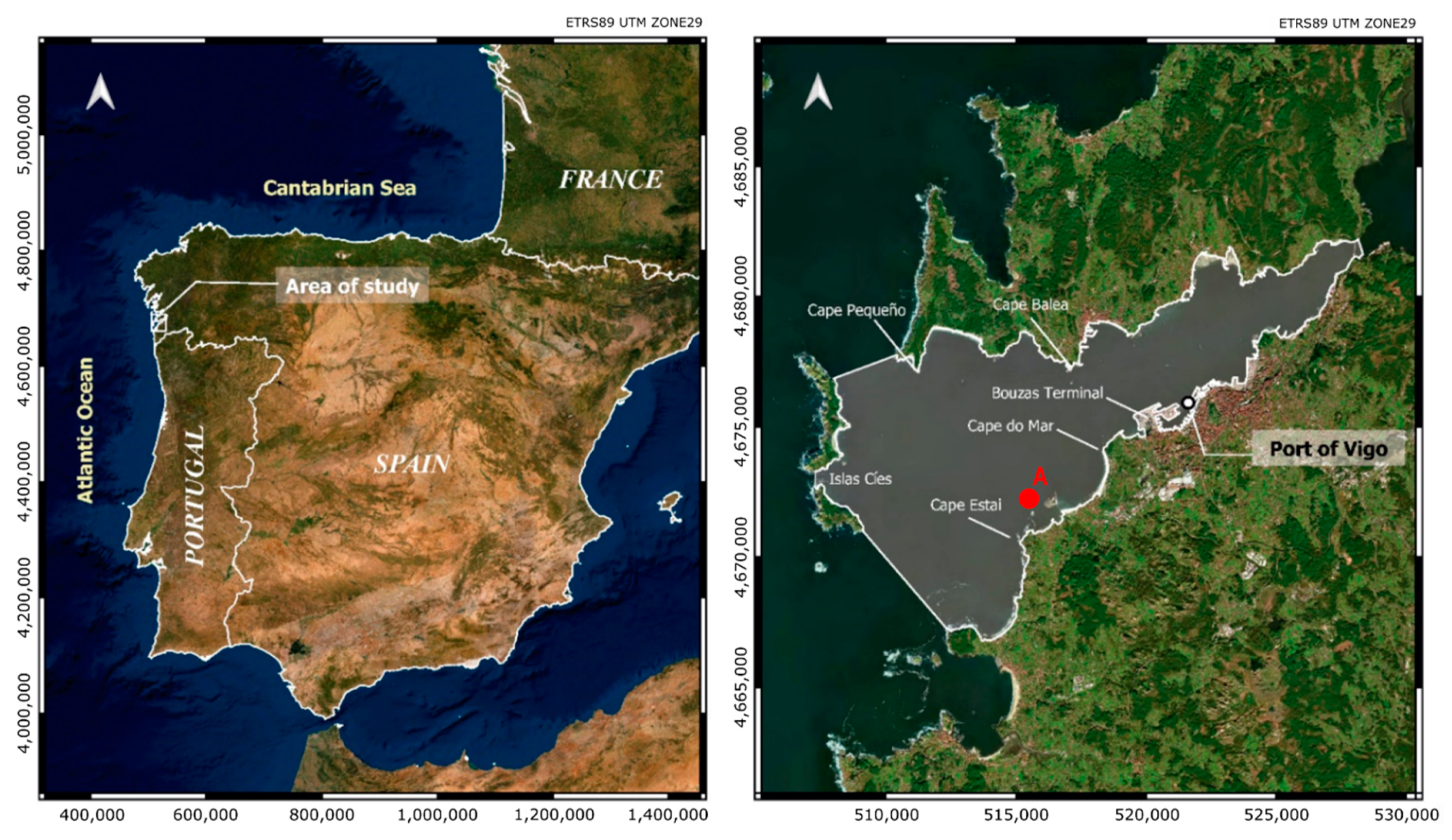
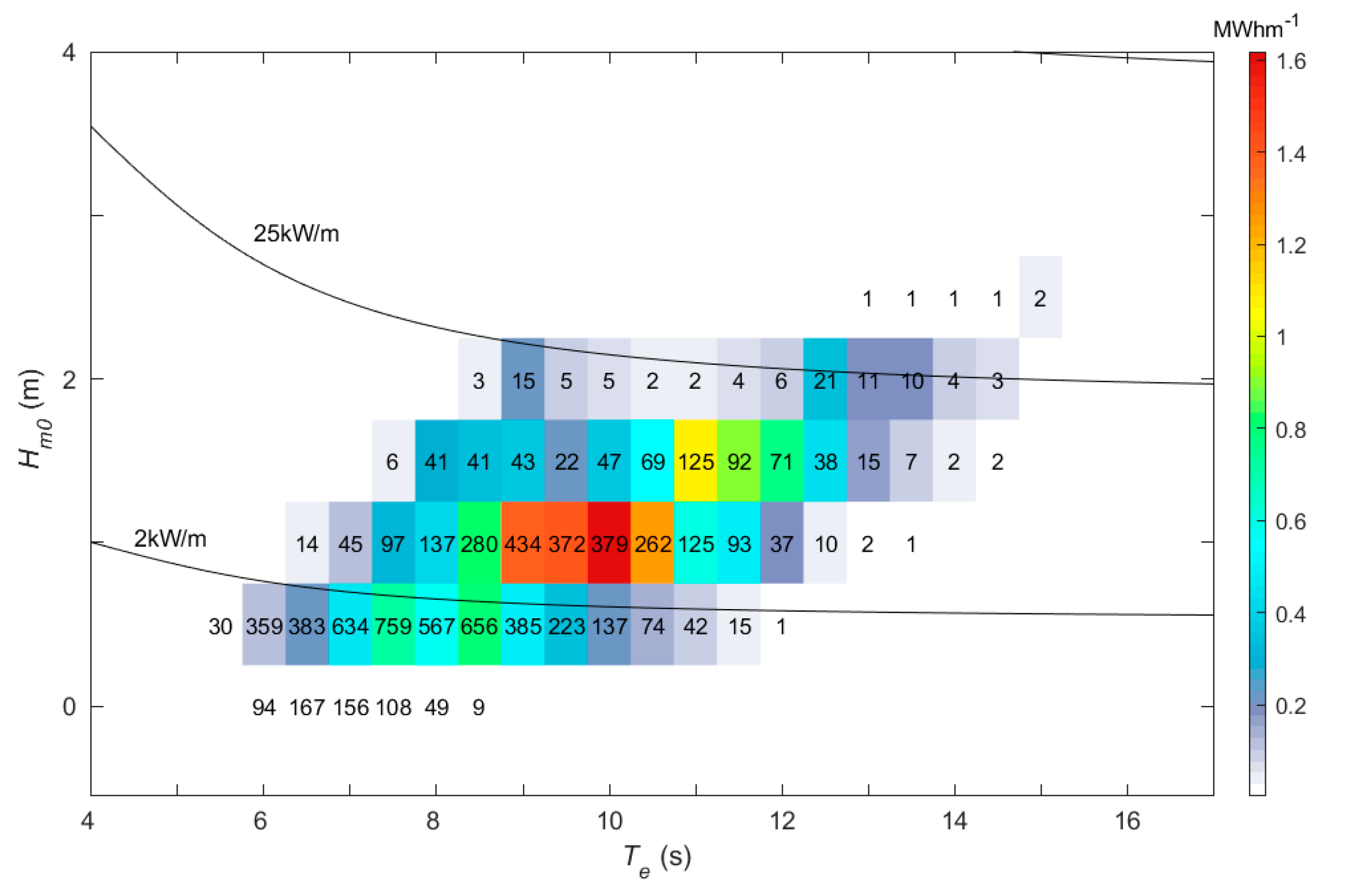
2.1. Case Study Site

The Port of Vigo (Figure 1) is one of the most important ports in the northwest of the Iberian Peninsula. It is located in the Ría de Vigo and constitutes a natural harbor that is sheltered by the Cíes Islands. In this port—as in many others—there is a growing interest in developing sustainable solutions which compensate for the high energy consumption and pollution emissions that take place on its operational areas. In this context, wave energy is one of the most important renewable energy sources at the Ría de Vigo area [29]. However, due to the natural protection that Cíes Islands provide, most of the port surroundings are wave sheltered areas. One of the most interesting locations is the zone near Cape Estai, just in front of a small island, named Toralla, off the south coast of the Ría, which is identify as Point A in Figure 1. The easting (X) and northing (Y) coordinates of this point are: X = 515,603 m, Y = 4,672,240 m (UTM29N/ETRS89). The reasons for selecting this area are mainly two: (i) it is one of the zones in the port surroundings with more available wave energy as it is exposed both to the northwest and southwest waves, that enter the Ría through the channels between the Cíes Islands and the north and south margins of the Ría; and (ii) an OWC wave energy converter at this location could provide shelter to Toralla Island, protecting it from the extreme wave events that often produce material damages to the facilities in the island.

The annual characterization matrix of the wave climate at Point A, discretized in terms of energy bins (bivariate intervals of spectral significant wave height and energy period), is presented in Figure 2. It can be seen that the sea states which provide the bulk of energy are those with significant wave heights around H_m0 = 1 m and energy periods around T_e = 10 s. Therefore, an OWC appropriate for being placed at this location should provide its best performance under wave conditions with these characteristics.

2.2. Numerical Modeling

In order to select the geometry of the OWC converter best suited for operating under the wave climate in the area of interest, a numerical wave flume—a mirror of the experimental wave flume at the University of Santiago de Compostela (USC)—was implemented. This approach has been followed in previous works both for the study of OWC wave energy converters [26,27] and other coastal engineering problems [30], obtaining excellent results. The numerical model used was OpenFOAM [31], an open source computational fluid dynamics (CFD) package organized as a series of toolboxes that encompass different numerical solvers, meshing tools and pre- and post-processing utilities.

2.2.1. Governing Equations

In order to take into account the effects of air compressibility—which is known to play a significant role in the performance of prototype OWC devices (e.g., [32])—the compressibleInterFoam solver was used. It is a pressure-based solver for two compressible, non-isothermal immiscible fluids using a volume-of-fluid interface capturing approach.

The governing equations are the mass (1), momentum (2) and energy (3) conservation equations, together with an equation of state (6) or (7):

$$\nabla ·\left(\rho u\right)+\frac{\partial \rho }{\partial t}=0 ,$$

(1)

$$\frac{\partial \rho u}{\partial t}+\nabla ·\left(\rho uu\right)=-\nabla p+\nabla ·\tau +\rho g+F ,$$

(2)

$$\frac{\partial \left(\rho C_p{T}_f\right)}{\partial t}+\nabla ·\left(\rho C_p{T}_{f}u\right)=\nabla \left({\mathsf{\Psi }}_e\nabla T_f\right)+S_T ,$$

(3)

where ρ is the fluid density; u is the fluid velocity vector; τ is the viscous stress tensor; g is the gravitational acceleration; p is the pressure; t is the time; F is the source of momentum due to surface tension; T_f is the temperature; C_p is the fluid specific heat; Ψ_e is the fluid thermal conductivity; and S_T is the source term in the energy equation.

The viscous stress tensor is:

$$\tau ={\mu }_{eff}\left[\nabla u+{\left(\nabla u\right)}^T\right]+\frac{2}{3}{\mu }_{eff}\left(\nabla ·u\right)I ,$$

(4)

where I is the identity tensor and μ_eff is the effective dynamic viscosity:

$${\mu }_{eff}=\mu +\rho {\nu }_{t },$$

(5)

where μ is the dynamic viscosity of the fluid and ν_t is the turbulent kinematic viscosity.

The equation of state for the air, which is assumed as a perfect gas, is:

$${\rho }_{air}=\frac{p}{R{T}_{f }},$$

(6)

where R is the specific gas constant. In the case of the water, a barotropic equation of state is used [33,34], defined as:

$${\rho }_{water}={\rho }_{water,0}+\psi p,$$

(7)

where ρ_water,0 is the initial reference water density; and ψ = 1/c² is an isothermal compressibility factor, with c being the speed of sound in water.

For the closure of the RANS equations, the k-omega-SST turbulence model [35] for compressible flow was adopted. For the capturing of the air–water interface, the volume-of-fluid (VOF) technique [36] was used. The VOF technique is a free surface tracking method that makes use of a phase-fraction function (α) which represents the fractional volume of a cell that is filled with water (e.g., α = 1 water, α = 0 air and 0 < α < 1 for an interfacial cell). Finally, the waves2Foam toolbox was used for wave generation [37]. It enables both the generation and (passive) absorption of waves based on the relaxation method.

2.2.2. Scaling

Given that the numerical model replicates the wave flume of the USC (with dimensions of 0.95 m high, 0.65 m wide and 20 m long) it is necessary to downscale the OWC designs in order to fit them in the numerical flume. Following previous works carried out in the flume of the USC [28,38,39], a 1:25 scale ratio was adopted.

When dealing with free surface flows—as in the case of a wave energy converter—the Froude number (ratio of inertia to gravity forces) in model and prototype must be maintained [40]. In addition, in the case of OWC devices, air compressibility effects inside the chamber are significant. Therefore, the ratio of the inertia to air compression forces must also be equal in model and prototype [41]. The best option for the simultaneous satisfaction of both ratios of forces is to make use of a conveniently shaped air chamber that satisfies the required scaling of the air chamber volume according to [42]:

$$\frac{V_m}{V_p}=\frac{1}{k_p}{\delta }^{-1}{\epsilon }^2 ,$$

(8)

where the subscripts m and p denote model and prototype, respectively; V is the air chamber volume in the absence of waves; k is the polytropic exponent of the full-size turbine, for which a value of k_p = 1.2 is assumed [42]; δ is the water density ratio (δ = ρ_m/ρ_p); and ε is the scale ratio (in this case ε = 1/25). For satisfying Equation (8) the air chamber was connected to an air reservoir of appropriate volume [28,42]. Details of the calculation of the air reservoir dimensions are presented in Appendix A.

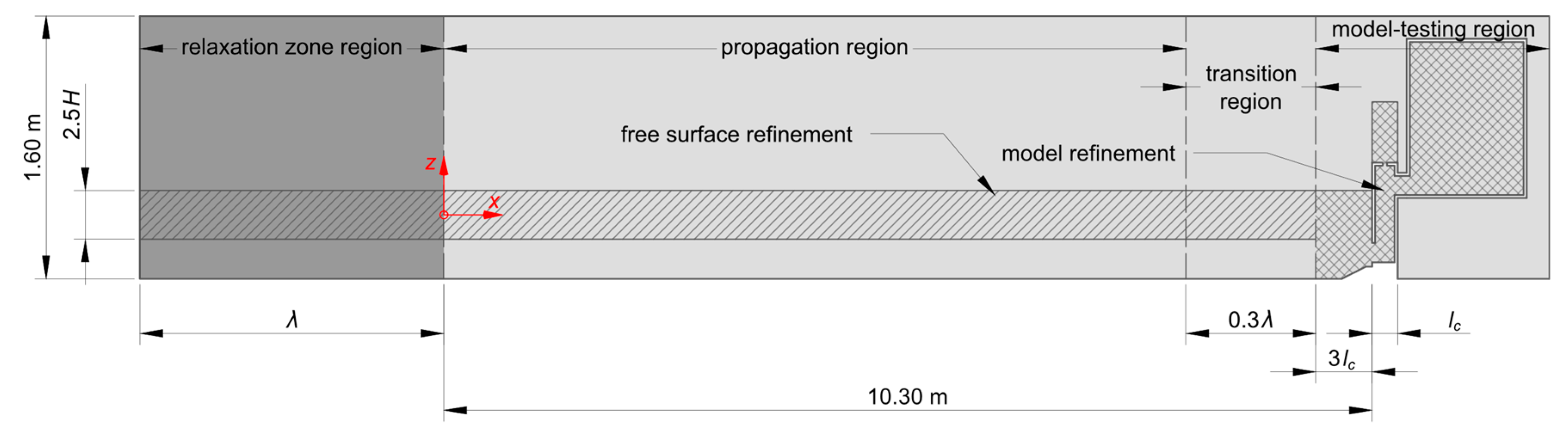
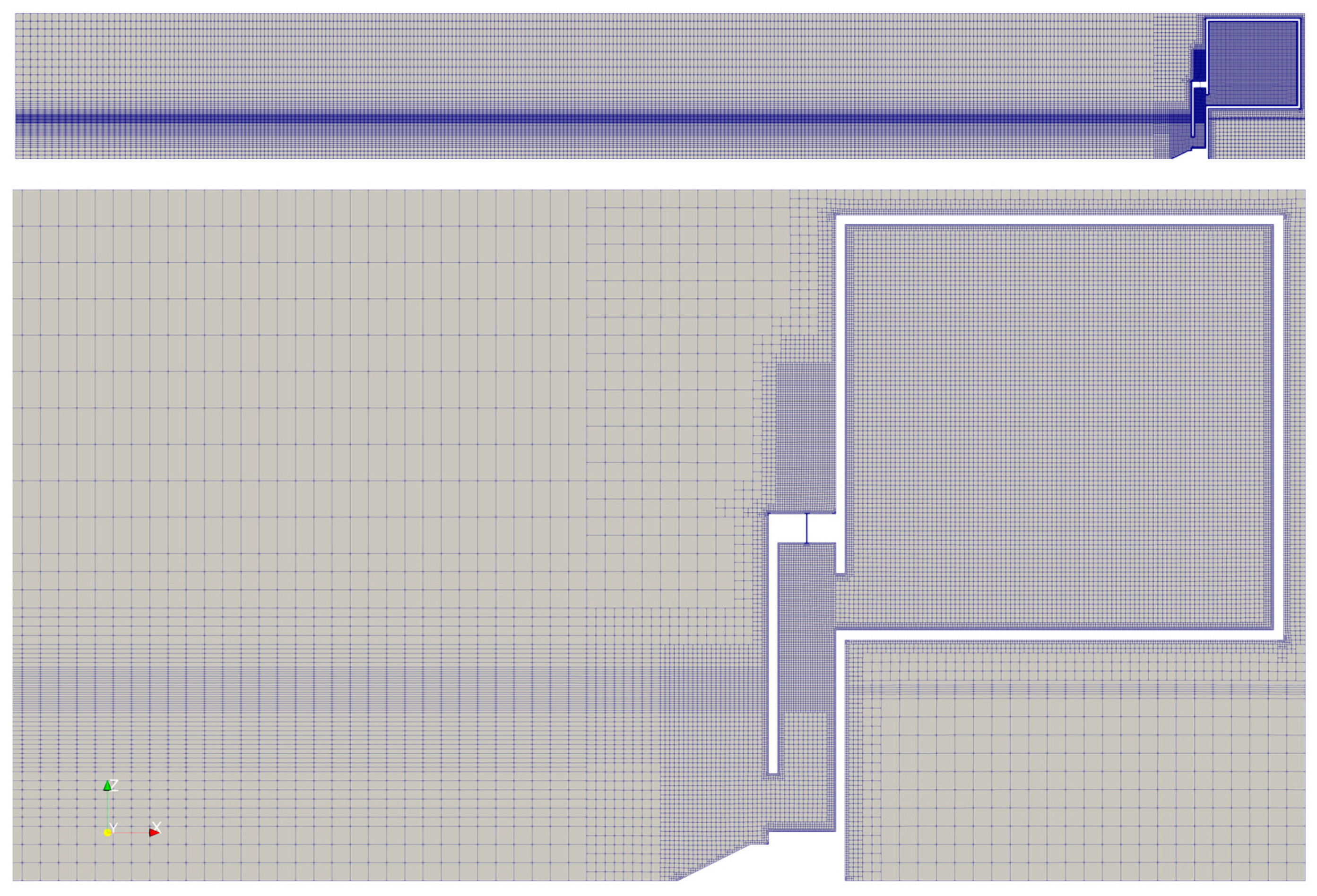
2.2.3. Computational Domain

As aforementioned, the computational domain reproduced the wave flume of the USC with the OWC model to be analyzed located at its end (Figure 3). In this case, a bidimensional set-up was considered. Thus, wave crests are assumed to be parallel to the OWC front wall. In order to implement the wave generation, an upstream relaxation zone of length equal to one wavelength was implemented. The air reservoir necessary to correctly consider the air compressibility effects was also reproduced in the numerical model.

The computational domain was discretized by means of the meshing tools blockMesh and snappyHexMesh available in the OpenFOAM package. First, a hexahedral base mesh was created using blockMesh. Second, snappyHexMesh was used to adapt the mesh to the OWC model surface by iteratively refining and morphing the base mesh. Four different mesh regions can be differentiated (Figure 3): (i) propagation region; (ii) relaxation zone region; (iii) transition region; and (iv) model-testing region.

The propagation region constitutes a meshing zone parametrized based on the wave conditions, i.e., its discretization changes depending on the wave condition to be simulated. It goes from x = 0 (end of the relaxation zone region) to the start of the transition region. In this section, the mesh is uniform along the x-axis, ensuring 50 cells per wavelength [43], and non-uniform along the z-axis, establishing a refined region in the vicinity of the air–water interface [26,28] that ensures H/Δz ≥ 8 [44]. The relaxation zone and the transition regions are, again, meshing zones parametrized based on the wave conditions. In the case of the relaxation zone region, its length is equal to the wavelength (λ) of each test [44,45]. Therefore, it goes from x = −λ to x = 0. The same cell size settings used for the propagation region were maintained with the exception of a growth rate that increase the cell size along the x‑axis towards the left wall of the model, established to help in the dissipation of reflected waves and to reduce the total number of cells. Regarding the transition region, its length is equal to 30% of the wavelength. It goes from the end of the propagation region to x = 10.30 m. The cell size settings in the transition region are the same of those in the propagation region except for a decreasing cell size along the x-axis towards the cell size in the next region. Finally, the model-testing region constitutes a non-parametrized meshing zone. It goes from the end of the transition region to the rear end of the air reservoir. Starting from a regular mesh of cell size 0.04 m, up to six refinement levels (minimum cell size of 6.25 × 10⁻⁴ m) were used to accommodate the shapes of the models. For illustration, the computational mesh for one of the wave conditions tested is presented in Figure 4.

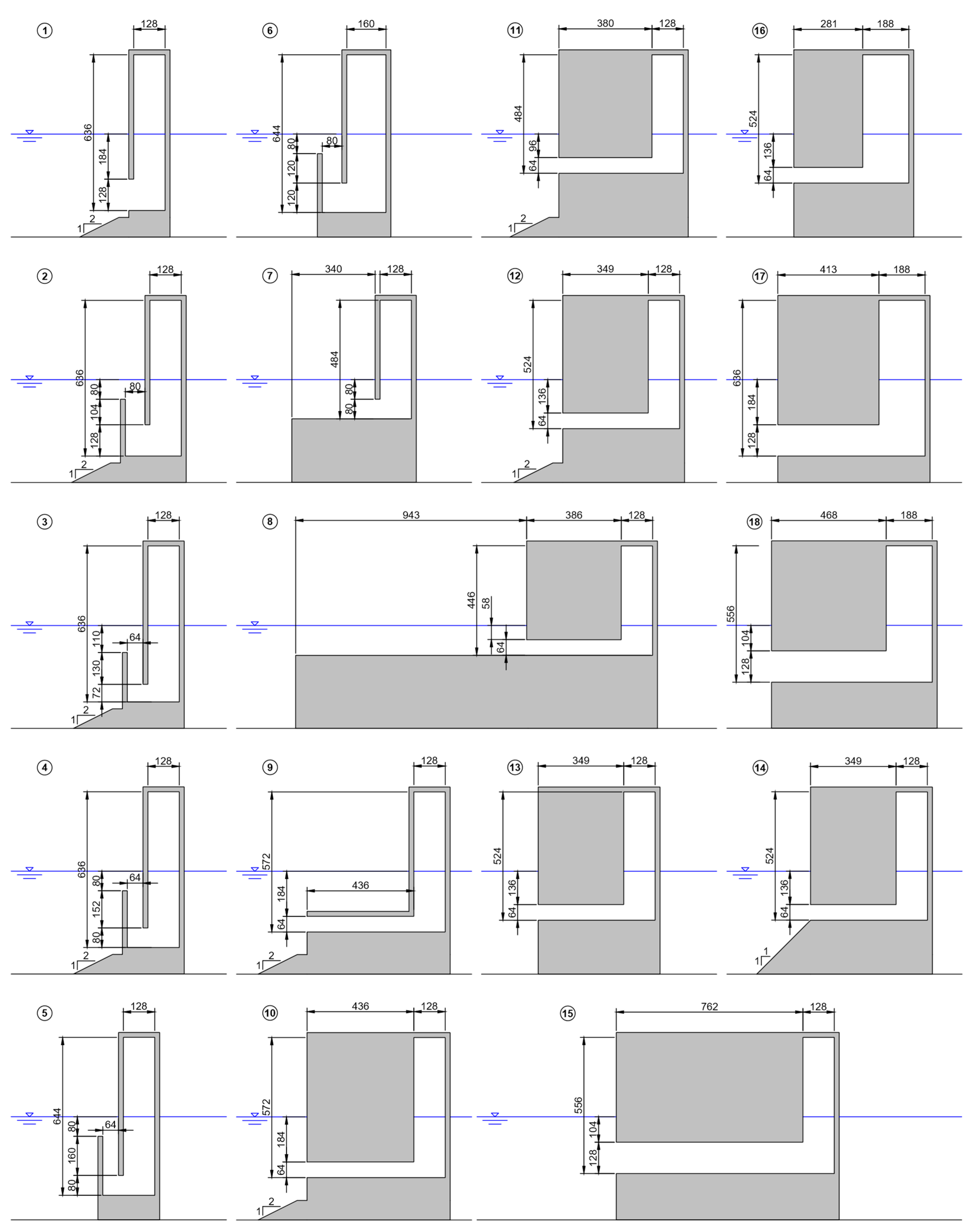
2.2.4. Testing Program

In total, 18 different OWC geometries were tested (Figure 5). The selected geometries were based on OWC configurations analyzed in previous studies, reproduced at a 1:25 scale. As mentioned, the design and dimensioning of these geometries follow two main criteria: (i) ease of integration into a coastal structure; and (ii) ease of construction. Model 1 represents a classic OWC design, intended for integration into the breakwater of the nearby Port of A Guarda (NW Spain) [27,46]. Models 2 to 6 are based on the U-shaped OWC [8]. The geometrical variants analyzed for the U-shaped designs encompass the width of the vertical duct, the submergence of the U-duct opening and the width of the chamber. Model 7 follows the stepped-bottom OWC design [9], and Model 8 combines the stepped and L‑shaped designs. Finally, Models 9 to 18 are L-shaped geometries [10,11]. In Model 10 the effects on the capture width ratio of a vertical wall added to the design to prevent wave transmission past the entrance of the OWC are analyzed. In Model 11 the influence of the depth of the entrance to the chamber on the performance of the device is analyzed. Through Models 12, 13 and 14 the influence on the capture width ratio of a sloping bed in front of the model is analyzed. Model 15 evaluates the effects on the efficiency of an L-shaped OWC of the height of the entrance to the chamber. Finally, Models 16, 17 and 18 enable the evaluation of the effects of the width (dimension orthogonal to the wave fronts) of the vertical duct and the depth of the entrance of the chamber on the performance of the device. For each of the designs studied the length of the water column was adjusted, to the extent possible, to achieve near-resonant conditions at the period of interest (T = 10 s).

The eighteen models were tested under six different regular wave conditions resulting from the combination of four wave periods T = 1.2, 1.6, 2.0 and 2.4 s (T = 6, 8, 10 and 12 s, in prototype dimensions) with a wave height of H = 0.04 m (H = 1 m, in prototype dimensions); plus two wave conditions with wave heights of H = 0.08 and 0.12 m and a wave period of T = 2.0 s (H = 2 and 3 m and T = 10 s, in prototype dimensions). The tests were carried out for a water depth of h = 0.42 m (h = 10.50 m, in prototype dimensions). Consequently, the wavelengths that correspond with the four tested periods, in order from smallest to largest, are λ = 1.96, 2.89, 3.77 and 4.63 m (λ = 49.06, 72.22, 94.31 and 115.81 m, in prototype dimensions). These wave conditions were selected based on the characterization matrix presented in Section 2.1.

The influence of the turbine on the system, i.e., the turbine-induced damping, was modelled by means of an orifice. As the numerical model is bidimensional, a rectangular orifice (slot) was used [26,47]. The flowrate through the slot (provided that turbulent flow is achieved) is proportional to the square-root of the pressure drop. For illustration, the data points of pressure drop versus flow rate for a tested case are presented in Figure 6 together with their corresponding fitted parabola of the form Δp/q² = const. It can be seen that there is a good agreement. The slot emulates, therefore, the behavior of non-linear air turbines such as the self-rectifying axial impulse or the biradial turbine, which present a quadratic pressure-drop-versus-flowrate relation [48]. Furthermore, given that the damping provided by these turbines is not significantly influenced by rotational speed changes [1], the slot appropriately simulates the damping of the turbine at different operating conditions. In this work, a slot of width w_s = 1.93 mm was used, a value which provides a pressure-drop-versus-flowrate relation that has shown good performance in previous works (e.g., [39]). By maintaining the slot width constant, the turbine-induced damping does not vary, i.e., it simulates the same the turbine for all the analyzed geometries. Note that better performance figures could be achieved if the turbine-chamber coupling is optimized.

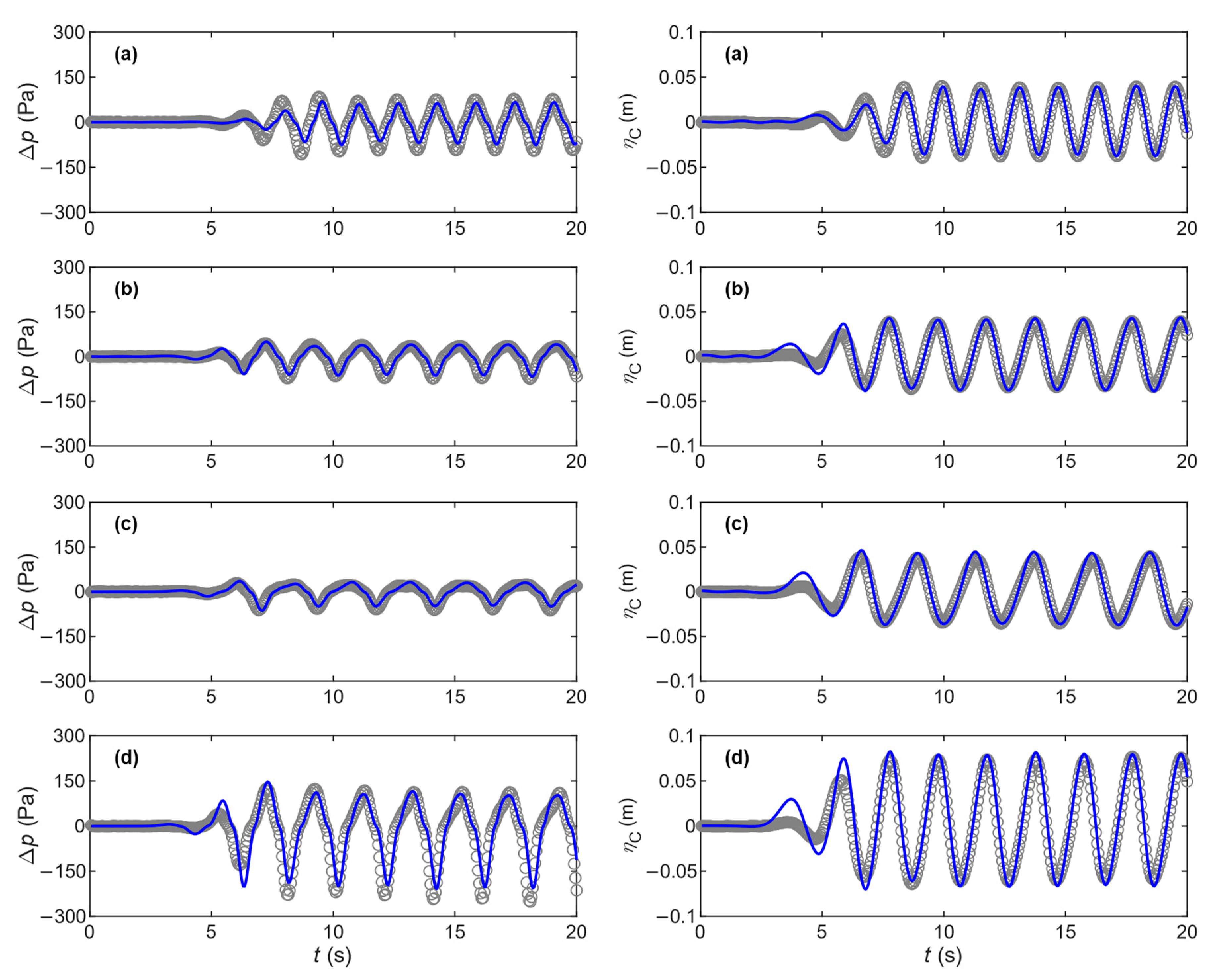
2.3. Numerical Model Validation

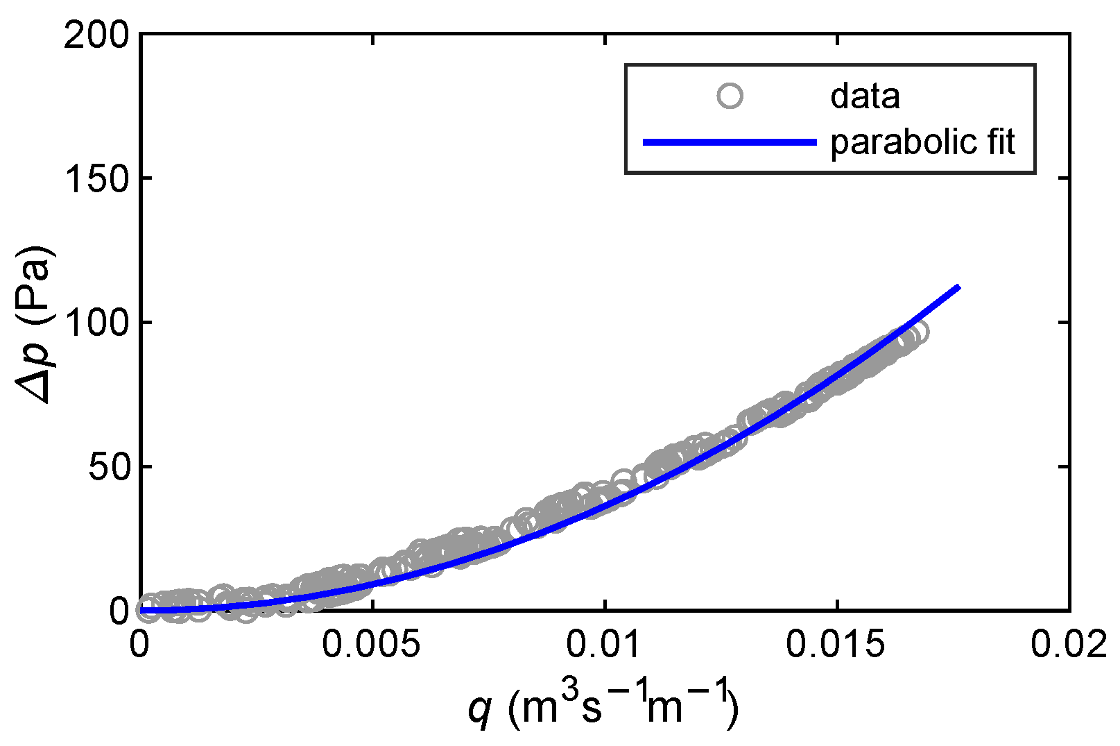
In order to validate the numerical model, the experimental data from López et al. [46] were used. Four wave conditions were considered: (a) H = 0.04 m, T = 1.6 s; (b) H = 0.04 m, T = 2.0 s; (c) H = 0.04 m, T = 2.4 s; and (d) H = 0.08 m, T = 2.0 s. The water depth was set to h = 0.42 m. The damping of the turbine was emulated by means of a slot of width w_s = 2.50 mm. A comprehensive description of the OWC model and the experimental set-up can be found in [46].

The time series of pressure drop between the interior of the chamber and the atmosphere and the oscillations of the water column inside the chamber are compared for both models, experimental and numerical, in Figure 7. For clarity, only the first 20 s of simulation are presented. In general, the agreement between both time series is excellent. The numerical model correctly reproduces the period and amplitude of the pressure drop and free surface elevation inside the chamber.

2.4. Data Analysis

The performance of the different OWC designs was characterized based on the capture-width ratio which is defined as:

$$C_{WR}=\frac{P_p}{w_c{P}_w} ,$$

(9)

where P_p is the pneumatic power; w_c is the width of the OWC chamber (direction parallel to the wave fronts); and P_w is the wave power per meter of wave front.

The pneumatic power is calculated as follows:

$$P_p=\frac{1}{t_{max}}{{\displaystyle \int }}_0^{t_{max}}\mathsf{\Delta }pQdt ,$$

(10)

where t_max is the time duration of each test; ∆p is the pressure drop between the interior of the OWC chamber and the atmosphere; and Q is the air flow rate through the orifice that emulates the turbine. Both variables, flowrate and pressure drop, were directly measured in the numerical model.

Finally, the wave power per meter of wave front is calculated as:

$$P_w=\frac{1}{8}{\rho }_{w}g{H}_i^2{C}_g ,$$

(11)

where ρ_w is the water density; H_i is the incident wave height; and C_g is the group velocity, calculated as:

$$C_g=\frac{1}{2}\frac{\sigma }{k}\left(1+\frac{2kh}{\sinh \left(2kh\right)}\right) ,$$

(12)

where σ and k are the wave angular frequency and the wave number, respectively, of the incident wave; and h is the water depth. The angular frequency is calculated from the dispersion relation as:

$${\sigma }^2=gk\tanh \left(kh\right) .$$

(13)

Furthermore, the response of the different OWC designs against the incident waves was characterized based on the response amplitude operator (RAO). The heave RAO of the water column oscillations is calculated as:

$$RA{O}_C=\frac{H_C}{H_i} ,$$

(14)

where H_C is the height of the water column oscillations. Additionally, the RAO of the pneumatic pressure oscillations is calculated, in its dimensionless form [16], as:

$$RA{O}_P=\frac{\Delta p_H}{{\rho }_{w}g{H}_i} ,$$

(15)

where Δp_H is the height of the pressure oscillations.

3. Results and Discussion

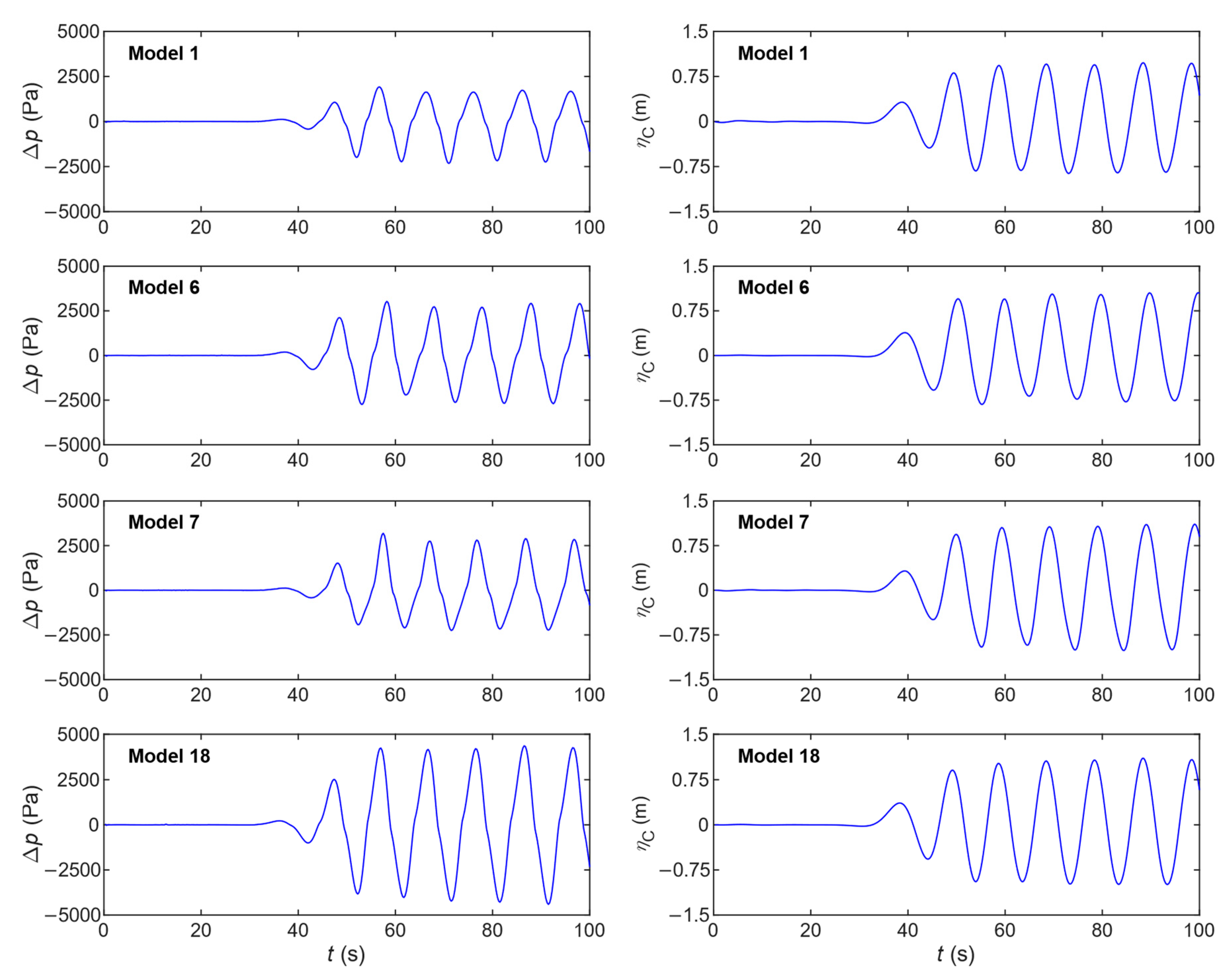
3.1. Response Analysis

The response of the oscillations of the water column and the pneumatic pressure oscillations inside the chamber (RAO_C and RAO_P, respectively) for the different OWC designs is presented in Figure 8. Furthermore, the maximum values of each operator for the different OWC geometries tested are summarized in

Table 1. Maximum values of (i) the response amplitude operator of the oscillations of the water column inside the chamber (RAO_C), (ii) and the response amplitude operator of the pressure oscillations (RAO_P), and (iii) the capture width ratio (C_WR), for the different OWC geometries tested (H = 1 m).

Model	RAOC, max	RAOP, max	CWR, max
1	2.07	0.63	0.597
2	2.39	0.57	0.357
3	2.54	0.58	0.295
4	2.49	0.58	0.294
5	2.53	0.60	0.310
6	2.22	0.64	0.356
7	2.45	0.62	0.429
8	2.87	0.82	0.479
9	2.59	0.55	0.254
10	3.36	0.78	0.450
11	3.23	0.74	0.444
12	3.17	0.74	0.454
13	3.16	0.74	0.453
14	3.26	0.78	0.490
15	3.43	0.97	0.667
16	2.39	0.82	0.494
17	2.50	0.97	0.695
18	2.52	0.99	0.716

. It can be seen that, in general, there are great variations on both operators depending on the wave frequency, higher in the case of the RAO_C (it ranges from 0.29 to 3.43) than in the RAO_P (it ranges from 0.05 to 0.99). The exception is Model 1, which presents a RAO_C nearly constant (around 2) for all the wave periods studied. In this model, the peak of the RAO_P is found for the lowest period and its value is below 0.70, showing that Model 1 is not performing well under the period of interest (T = 10 s). The best OWC design in terms of amplitude operators is the L‑shaped (Models 9 to 18), in particular, Models 11 to 18 stand out with values of the RAO_P over 0.70 for the period of interest. Among the different L‑shaped geometries, Models 15, 17 and 18 are the best ones, with values of the RAO_P for the period of interest of 0.97, 0.97 and 0.99, respectively. Interestingly, these models do not present the highest figures of the RAO_C, which, for the period of interest, are achieved by Models 14 and 15 (RAO_C = 3.02 and 3.13, respectively), which is related to the wider chamber of Models 17 and 18. The different behavior showed by the two operators emphasizes the importance of considering both of them, although, as it can be verified in Table 1 by comparing with the values of the capture-width ratio, the operator that best captures the OWC performance is the RAO_P.

Although the U-shaped designs (Models 2 to 6) perform better than Model 1, they do not offer response amplitudes comparable to those of the L-shaped geometries. They are well tuned, with the maximum values of the RAOs achieved for the period of interest, but the values of the RAO_P are in all the cases below 0.70. The best U-shaped design in terms of the RAO_P is Model 6 and, again, as a model with a wider chamber, it does not present high values of the RAO_C when compared with the remaining U-shaped models. The stepped-bottom version of the classic design (Model 7) improves the response of Model 1 but only on the higher periods. In this model, the maximum value of the pressure amplitude operator is RAO_P = 0.62 and it is achieved for T = 8 s. Finally, the stepped version of the L-shaped design (Model 8) follows similar trends than those of the original L‑shaped designs, indicating that the presence of the step does not improve the performance of the system in this case.

Finally, the time series of pressure drop and free surface elevation within the chamber are presented for Models 1, 6, 7 and 18, as representative of the four general shapes analyzed in this work: classic, stepped-bottom, U-shaped and L-shaped, respectively (Figure 9). It can be seen that the response amplitude operators adequately capture the response of the different OWC designs to the incident waves.

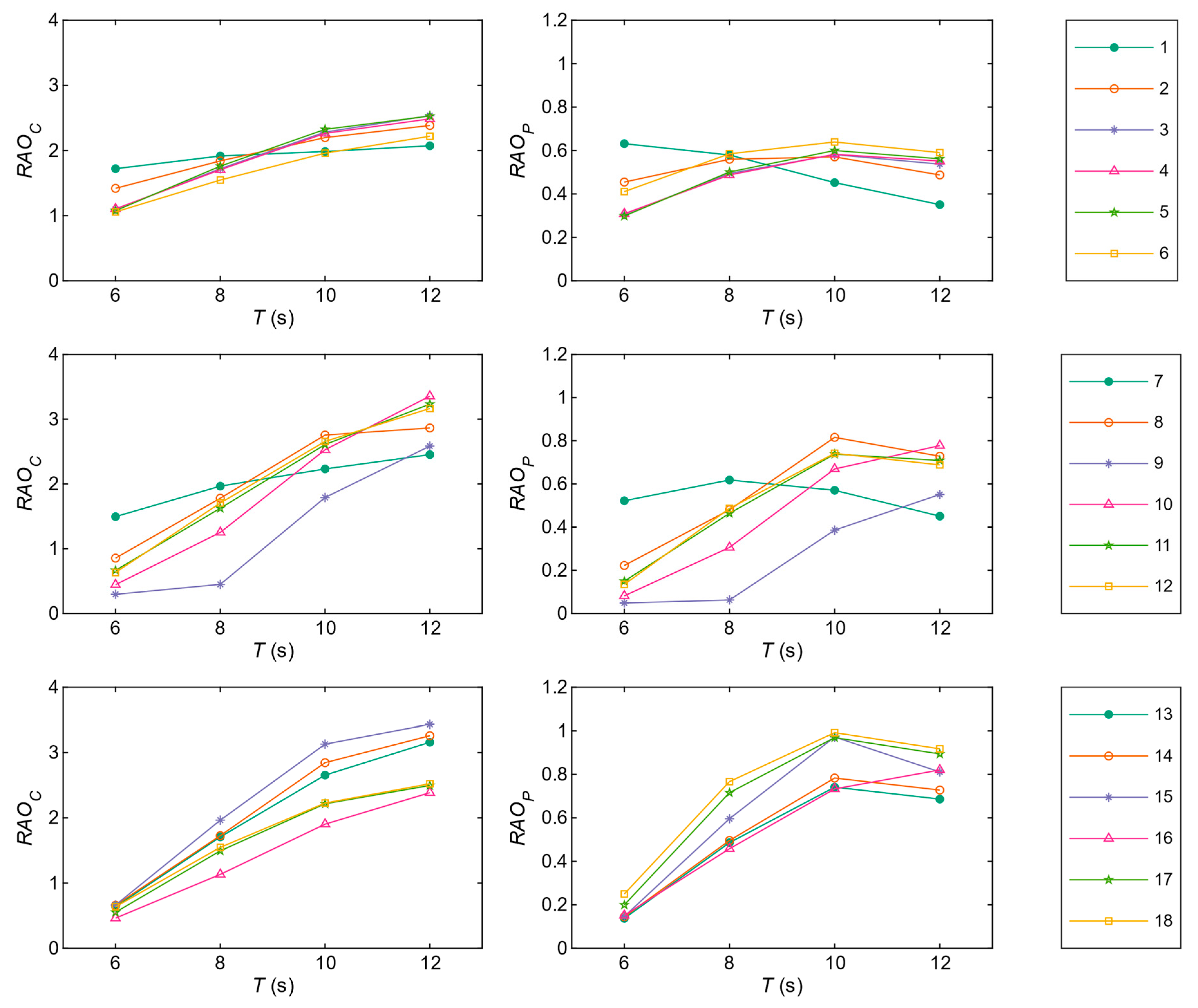
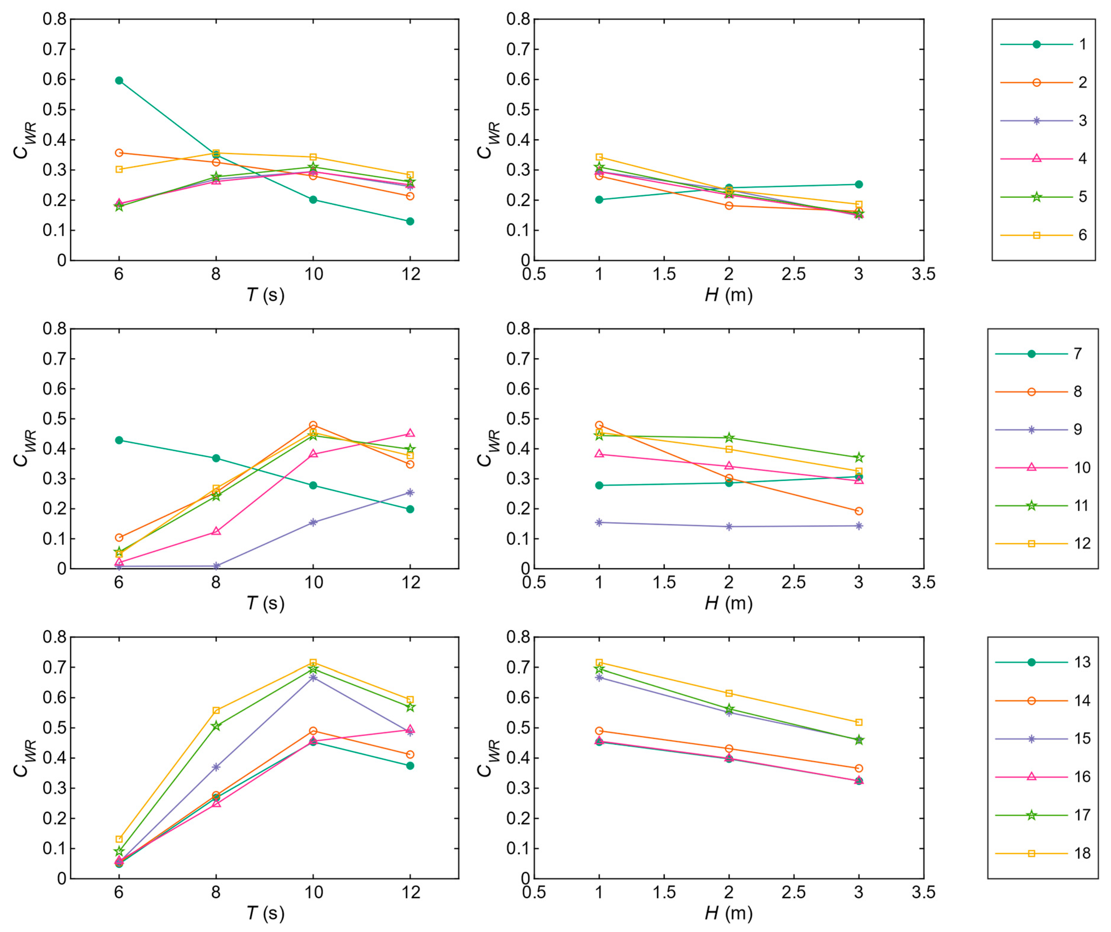
3.2. Performance of the OWC Geometries

The values of the capture-width ratio for the different geometries tested are presented in Figure 10 and its maximum values are summarized in Table 1. The classic OWC design (Model 1) provides the highest value of the capture-width ratio (C_WR = 0.597) for the smallest period of the four tested (T = 6 s). For T = 10 s the capture-width ratio is comparatively lower (C_WR = 0.202). Interestingly, when the wave height increases, the performance of Model 1 under T = 10 s increases too, up to C_WR = 0.252. This result, albeit an exception among the different OWC models tested, is in line with the conclusions achieved in [46] for the same OWC design. Given that, as presented in Section 2.1, the bulk of the wave energy in the area of interest is provided by sea states with energy period around 10 s, Model 1 can be disregarded due to its too low resonant period. Furthermore, the classic OWC design constitutes a very rigid geometry, as there is little place for adapting the resonant frequency of the OWC model to match that of the incident waves. In fact, the only possibility to reduce the resonant frequency of the system (move it to higher periods) is to increase the height of the water column by moving the entrance towards the sea bottom; this solution is, however, limited by the water depth.

The U-shaped OWC designs (Models 2–6) present lower maximum values of the capture-width ratio (C_WR = 0.294–0.357) than the classic OWC design (C_WR = 0.597). However, these maximum values of the capture-width ratio are achieved (with the exception of Model 2) for periods closer to T = 10 s, so constituting a better design for being installed in the study area. In addition, the U-shaped designs present a smoother performance when working out of the resonant period, in the sense that the variability in the values of the capture-width ratio is lower than that of the classic design. Thus, for the U-shaped designs the capture-width ratio varies for wave conditions with H = 1 m between C_WR = 0.179 and C_WR = 0.357, whereas for the classic design it varies between C_WR = 0.597 and C_WR = 0.130. Among the five U-shaped OWC geometries, the best one is Model 6, with a capture-width ratio of C_WR = 0.343 for T = 10 s, and values above C_WR = 0.284 for the other periods analyzed. The main distinctive characteristic in this model from the other U‑shaped designs is a wider chamber.

Model 7 constitutes the stepped-bottom version of the classic OWC design. The results showed that in comparison with the classic OWC design, the stepped-bottom version increases the performance range of the device in the sense that the values of the capture-width ratio are higher for the wave conditions with periods different from the resonant one, but at the expense of reducing the maximum capture-width ratio. Thus, in Model 7 the highest value of the capture-width ratio, achieved for T = 6 s, is C_WR = 0.429, whereas in Model 1, also achieved for T = 6 s, it is C_WR = 0.597. On the contrary, for T = 8, 10 and 12 s the values of capture-width ratio for Model 7 are C_WR = 0.369, 0.278 and 0.198, respectively, whereas for Model 1 they are C_WR = 0.350, 0.202 and 0.130, respectively. As in the case of the classic design, the tuning of the resonant period in the stepped-bottom design is not straightforward because the main resonance mechanism due to the natural frequency of oscillation of the water column is, again, limited by the height of the water column [9]. In an attempt to overcome this limitation, the stepped and L‑shaped designs were combined in Model 8. This solution, though, did not significantly improve the performance of the L‑shaped designs and showed low performance figures for the wave conditions with higher wave heights.

The results from Models 9 to 18 correspond with the L-shaped designs. The two first L-shaped geometries, Model 9 and 10, present a resonant period closer to T = 12 s than to T = 10 s. However, despite being slightly out of tune, these two models show that having a vertical wall to avoid waves going beyond the entrance of the OWC significantly improves the performance of an L‑shaped device. For example, for T = 10 s the capture-width ratio of Model 9 (C_WR = 0.154) is increased up to C_WR = 0.382 when the vertical wall is located just at the entrance of the device. Based on this result, all the remaining models were based on the design of Model 10. Model 11 was designed to better match the resonant period of interest (T = 10 s). It provides a maximum capture-width ratio of C_WR = 0.444 for T = 10 s. In addition, the capture-width ratio presents higher figures in the whole range of the wave conditions analyzed. Model 12 slightly improves the matching of the resonant period of the chamber with the period of interest by increasing the depth of the entrance and reducing the length of the horizontal section of the chamber. It provides a maximum capture-width ratio of C_WR = 0.454 for T = 10 s. Nevertheless, for T = 12 s and especially for H = 2 and 3 m, the performance of Model 12 is lower than that of Model 11. This situation is related with the deeper entrance, as it will be shown below.

The influence of a sloping bed was analyzed in Models 12, 13 and 14. Whereas the presence of a traditional bedding layer (in the same way as in the case of a vertical breakwater), as that in Model 12, virtually does not affect the performance of the device when comparing with a device without sloping bed as in the case of Model 13 (capture-width ratio for T = 10 s of C_WR = 0.454 and 0.453, respectively), an oversized bedding layer as the presented in Model 14 slightly improves its performance (C_WR = 0.490 for T = 10 s). In any case, the improvement is not significant and implies a cost overrun that could not justify its use. In Model 15, the influence of the height of the entrance of the chamber is analyzed. The improvements in this case are substantial. Thus, when comparing Model 15 with Model 14, the values of the capture-width ratio increase for all the wave conditions tested, with a considerable improvement (above 35%) for the wave conditions with T = 10 s and H = 1 m. The disadvantage in this design is that, for maintaining the matching between the natural period of the chamber and the period of interest, the length of the horizontal section has to be increased up to 20.65 m (82.6 cm in model dimensions).

The more feasible solutions for reducing the length of the horizontal section of the chamber while maintaining its natural period close to 10 s are: (i) to increase the width (dimension orthogonal to the wave fronts) of the vertical duct of the chamber; and (ii) to increase the depth of the entrance of the chamber. These two modifications are analyzed through Models 16, 17 and 18. Model 16 is equivalent to Model 13, but with a wider vertical duct. It can be seen that the differences between the values of the capture-width ratio of both models are small or, as in the case of a wave condition with T = 12 s and H = 1 m, positive for the model with the wider vertical duct. Similarly, Model 18 is equivalent to Model 15, but with a wider vertical duct. Again, although the maximum value of the capture-width ratio in Model 18 (C_WR = 0.716) is similar to that of the thinner-duct model, there is a significant increase in the values of the capture-width ratio for the wave conditions with T = 8 s and T = 12 s. Finally, the influence of the submergence of the entrance of the chamber (the distance from the water free surface to the device entrance) was studied through Model 17, that is equivalent to Model 18, but with a deeper horizontal duct. For all the wave conditions studied, the shallower duct captures more energy than the deeper one.

4. Conclusions

In this work, different OWC wave energy converter designs were analyzed for determining the best performing geometry when operating under a given wave climate at a given location. Four general designs of OWC were analyzed: classic, stepped-bottom, U-shaped and L-shaped, and considering for each of them a number of geometrical variants. To this end, a numerical model based on the Navier-Stokes equations for two compressible fluids was implemented with a volume-of-fluid interface-capturing approach and the waves2Foam toolbox for wave generation. The work was illustrated through a case study in the surroundings of the Port of Vigo (NW Spain).

It was found that the classic and stepped-bottom designs constitute rigid geometries, in the sense that there is little room for adjusting their natural period of oscillation to the desired one—the only adjustment possibility is to lower or raise the entrance of the chamber to modify the length of the water column. Whereas the classic OWC design suffers from a narrow period performance range, the stepped-bottom design, thanks to its multiple resonance mechanisms, presents high values of the capture-width ratio for a wide range of periods. On the other hand, the U-shaped and L-shaped designs are easy to tune thanks to the particular configuration of the chamber that enables significant adjustments in the length of the water column to be made. Overall, the best OWC design is the L-shaped, which improves the performance of the other configurations (classic, U-shaped and stepped-bottom) for two reasons: (i) its performance and response amplitude operators (RAO_C and RAO_P) within the range of periods of interest are the highest of all the configurations analyzed; and (ii) its natural period of oscillation matches—or, rather, can be tuned to match—that providing the bulk of energy at the location of interest.

Regarding the geometric modifications that can be made for improving the performance of an L‑shaped design the following conclusions can be drawn. First, a wider vertical section of the chamber (in the dimension orthogonal to the wave fronts) improves the performance of the device by increasing the values of the capture-width ratio mainly for periods different from the natural period of oscillation of the chamber. Second, the greater the height of the horizontal duct of the chamber (the entrance), the higher the captured energy. Third, a shallower entrance is positive from the efficiency point of view.

In conclusion, of the different OWC designs suitable for a structure-integrated device, the L‑shaped geometry is shown to provide the best performance and allow greater flexibility to be tuned for resonance at the desired period. Further research involving irregular wave conditions and different values of the turbine-induced damping will be conducted in future works.

References

1. Falcão, A.F.O.; Henriques, J.C.C. Oscillating-water-column wave energy converters and air turbines: A review. Renew. Energy 2016, 85, 1391–1424. [Google Scholar] [CrossRef]
2. Falcão, A.F.O.; Henriques, J.C.C.; Gato, L.M.C. Self-rectifying air turbines for wave energy conversion: A comparative analysis. Renew. Sustain. Energy Rev. 2018, 91, 1231–1241. [Google Scholar] [CrossRef]
3. Rajapakse, G.; Jayasinghe, S.; Fleming, A. Power Smoothing and Energy Storage Sizing of Vented Oscillating Water Column Wave Energy Converter Arrays. Energies 2020, 13, 1278. [Google Scholar] [CrossRef] [Green Version]
4. Kumar, P.M.; Halder, P.; Husain, A.; Samad, A. Performance enhancement of Wells turbine: Combined radiused edge blade tip, static extended trailing edge, and variable thickness modifications. Ocean Eng. 2019, 185, 47–58. [Google Scholar] [CrossRef]
5. Luo, Y.; Presas, A.; Wang, Z. Numerical Analysis of the Influence of Design Parameters on the Efficiency of an OWC Axial Impulse Turbine for Wave Energy Conversion. Energies 2019, 12, 939. [Google Scholar] [CrossRef] [Green Version]
6. Elatife, K.; El Marjani, A. Efficiency improvement of a self-rectifying radial impulse turbine for wave energy conversion. Energy 2019, 189, 116257. [Google Scholar] [CrossRef]
7. Falcão, A.F.O.; Gato, L.M.C.; Nunes, E.P.A.S. A novel radial self-rectifying air turbine for use in wave energy converters. Renew. Energy 2013, 50, 289–298. [Google Scholar] [CrossRef]
8. Boccotti, P. Comparison between a U-OWC and a conventional OWC. Ocean Eng. 2007, 34, 799–805. [Google Scholar] [CrossRef]
9. Rezanejad, K.; Bhattacharjee, J.; Soares, C.G. Stepped sea bottom effects on the efficiency of nearshore oscillating water column device. Ocean Eng. 2013, 70, 25–38. [Google Scholar] [CrossRef]
10. Howe, D.; Nader, J.R. OWC WEC integrated within a breakwater versus isolated: Experimental and numerical theoretical study. Int. J. Mar. Energy 2017, 20, 165–182. [Google Scholar] [CrossRef]
11. Rezanejad, K.; Souto-Iglesias, A.; Guedes Soares, C. Experimental investigation on the hydrodynamic performance of an L-shaped duct oscillating water column wave energy converter. Ocean Eng. 2019, 173, 388–398. [Google Scholar] [CrossRef]
12. Cabral, T.; Clemente, D.; Rosa-Santos, P.; Taveira-Pinto, F.; Morais, T.; Belga, F.; Cestaro, H. Performance Assessment of a Hybrid Wave Energy Converter Integrated into a Harbor Breakwater. Energies 2020, 13, 236. [Google Scholar] [CrossRef] [Green Version]
13. Zheng, S.; Zhu, G.; Simmonds, D.; Greaves, D.; Iglesias, G. Wave power extraction from a tubular structure integrated oscillating water column. Renew. Energy 2020, 150, 342–355. [Google Scholar] [CrossRef]
14. Zhou, Y.; Zhang, C.; Ning, D. Hydrodynamic Investigation of a Concentric Cylindrical OWC Wave Energy Converter. Energies 2018, 11, 985. [Google Scholar] [CrossRef] [Green Version]
15. Wan, C.; Yang, C.; Fang, Q.; You, Z.; Geng, J.; Wang, Y. Hydrodynamic Investigation of a Dual-Cylindrical OWC Wave Energy Converter Integrated into a Fixed Caisson Breakwater. Energies 2020, 13, 896. [Google Scholar] [CrossRef] [Green Version]
16. Perez-Collazo, C.; Greaves, D.; Iglesias, G. A Novel Hybrid Wind-Wave Energy Converter for Jacket-Frame Substructures. Energies 2018, 11, 637. [Google Scholar] [CrossRef] [Green Version]
17. Zheng, S.; Zhang, Y.; Iglesias, G. Power capture performance of hybrid wave farms combining different wave energy conversion technologies: The H-factor. Energy 2020, 204, 117920. [Google Scholar] [CrossRef]
18. Cui, L.; Zheng, S.; Zhang, Y.; Miles, J.; Iglesias, G. Wave power extraction from a hybrid oscillating water column-oscillating buoy wave energy converter. Renew. Sustain. Energy Rev. 2021, 135, 110234. [Google Scholar] [CrossRef]
19. Gaspar, L.A.; Teixeira, P.R.F.; Didier, E. Numerical analysis of the performance of two onshore oscillating water column wave energy converters at different chamber wall slopes. Ocean Eng. 2020, 201, 107119. [Google Scholar] [CrossRef]
20. Raj, D.; Sundar, V.; Sannasiraj, S.A. Enhancement of hydrodynamic performance of an Oscillating Water Column with harbour walls. Renew. Energy 2019, 132, 142–156. [Google Scholar] [CrossRef]
21. Zheng, S.; Antonini, A.; Zhang, Y.; Miles, J.; Greaves, D.; Zhu, G.; Iglesias, G. Hydrodynamic performance of a multi-Oscillating Water Column (OWC) platform. Appl. Ocean Res. 2020, 99, 102168. [Google Scholar] [CrossRef]
22. Zheng, S.; Antonini, A.; Zhang, Y.; Greaves, D.; Miles, J.; Iglesias, G. Wave power extraction from multiple oscillating water columns along a straight coast. J. Fluid Mech. 2019, 878, 445–480. [Google Scholar] [CrossRef]
23. Shih, H.-J.; Chang, C.-H.; Chen, W.-B.; Lin, L.-Y. Identifying the Optimal Offshore Areas for Wave Energy Converter Deployments in Taiwanese Waters Based on 12-Year Model Hindcasts. Energies 2018, 11, 499. [Google Scholar] [CrossRef] [Green Version]
24. Su, W.R.; Chen, H.; Chen, W.B.; Chang, C.H.; Lin, L.Y.; Jang, J.H.; Yu, Y.C. Numerical investigation of wave energy resources and hotspots in the surrounding waters of Taiwan. Renew. Energy 2018, 118, 814–824. [Google Scholar] [CrossRef]
25. Carballo, R.; Arean, N.; Álvarez, M.; López, I.; Castro, A.; López, M.; Iglesias, G. Wave farm planning through high-resolution resource and performance characterization. Renew. Energy 2019, 135, 1097–1107. [Google Scholar] [CrossRef]
26. López, I.; Pereiras, B.; Castro, F.; Iglesias, G. Optimisation of turbine-induced damping for an OWC wave energy converter using a RANS-VOF numerical model. Appl. Energy 2014, 127, 105–114. [Google Scholar] [CrossRef]
27. López, I.; Pereiras, B.; Castro, F.; Iglesias, G. Holistic performance analysis and turbine-induced damping for an OWC wave energy converter. Renew. Energy 2016, 85, 1155–1163. [Google Scholar] [CrossRef]
28. López, I.; Carballo, R.; Taveira-Pinto, F.; Iglesias, G. Sensitivity of OWC performance to air compressibility. Renew. Energy 2020, 145, 1334–1347. [Google Scholar] [CrossRef]
29. Iglesias, G.; Carballo, R. Choosing the site for the first wave farm in a region: A case study in the Galician Southwest (Spain). Energy 2011, 36, 5525–5531. [Google Scholar] [CrossRef]
30. López, I.; Rosa-Santos, P.; Moreira, C.; Taveira-Pinto, F. RANS-VOF modelling of the hydraulic performance of the LOWREB caisson. Coast. Eng. 2018, 140, 161–174. [Google Scholar] [CrossRef]
31. Jasak, H.; Jemcov, A.; Tukovic, Z. OpenFOAM: A C++ library for complex physics simulations. In Proceedings of the International Workshop on Coupled Methods in Numerical Dynamics, Dubrovnik, Croatia, 19–21 September 2007; pp. 1–20. [Google Scholar]
32. Falcão, A.F.O.; Henriques, J.C.C. The spring-like air compressibility effect in oscillating-water-column wave energy converters: Review and analyses. Renew. Sustain. Energy Rev. 2019, 112, 483–498. [Google Scholar] [CrossRef]
33. Martínez Ferrer, P.J.; Causon, D.M.; Qian, L.; Mingham, C.G.; Ma, Z.H. A multi-region coupling scheme for compressible and incompressible flow solvers for two-phase flow in a numerical wave tank. Comput. Fluids 2016, 125, 116–129. [Google Scholar] [CrossRef] [Green Version]
34. Seiffert, B.R.; Ertekin, R.C.; Robertson, I.N. Wave loads on a coastal bridge deck and the role of entrapped air. Appl. Ocean Res. 2015, 53, 91–106. [Google Scholar] [CrossRef]
35. Menter, F.R.; Kuntz, M.; Langtry, R. Ten years of industrial experience with the SST turbulence model. Turbul. Heat Mass Transf. 2003, 4, 625–632. [Google Scholar]
36. Hirt, C.W.; Nichols, B.D. Volume of fluid (VOF) method for the dynamics of free boundaries. J. Comput. Phys. 1981, 39, 201–225. [Google Scholar] [CrossRef]
37. Jacobsen, N.G.; Fuhrman, D.R.; Fredsøe, J. A wave generation toolbox for the open-source CFD library: OpenFoam®. Int. J. Numer. Methods Fluids 2012, 70, 1073–1088. [Google Scholar] [CrossRef]
38. López, I.; Carballo, R.; Iglesias, G. Site-specific wave energy conversion performance of an oscillating water column device. Energy Convers. Manag. 2019, 195, 457–465. [Google Scholar] [CrossRef]
39. López, I.; Carballo, R.; Iglesias, G. Intra-annual variability in the performance of an oscillating water column wave energy converter. Energy Convers. Manag. 2020, 207, 112536. [Google Scholar] [CrossRef]
40. Hughes, S.A. Physical Models and Laboratory Techniques in Coastal Engineering; World Scientific: Singapore, 1993; Volume 7, ISBN 981-02-1540-1. [Google Scholar]
41. Weber, J. Representation of non-linear aero-thermodynamic effects during small scale physical modelling of OWC WECs. In Proceedings of the 7th European Wave and Tidal Energy Conference (EWTEC), Porto, Portugal, 11–13 September 2007; pp. 11–14. [Google Scholar]
42. Falcão, A.F.O.; Henriques, J.C.C. Model-prototype similarity of oscillating-water-column wave energy converters. Int. J. Mar. Energy 2014, 6, 18–34. [Google Scholar] [CrossRef]
43. Vanneste, D.; Troch, P. 2D numerical simulation of large-scale physical model tests of wave interaction with a rubble-mound breakwater. Coast. Eng. 2015, 103, 22–41. [Google Scholar] [CrossRef]
44. Simonetti, I.; Cappietti, L.; Elsafti, H.; Oumeraci, H. Optimization of the geometry and the turbine induced damping for fixed detached and asymmetric OWC devices: A numerical study. Energy 2017, 139, 1197–1209. [Google Scholar] [CrossRef]
45. Hu, Z.Z.; Greaves, D.; Raby, A. Numerical wave tank study of extreme waves and wave-structure interaction using OpenFoam®. Ocean Eng. 2016, 126, 329–342. [Google Scholar] [CrossRef] [Green Version]
46. López, I.; Pereiras, B.; Castro, F.; Iglesias, G. Performance of OWC wave energy converters: Influence of turbine damping and tidal variability. Int. J. Energy Res. 2015, 39, 472–483. [Google Scholar] [CrossRef]
47. Zhang, Y.; Zou, Q.-P.; Greaves, D. Air-water two-phase flow modelling of hydrodynamic performance of an oscillating water column device. Renew. Energy 2012, 41, 159–170. [Google Scholar] [CrossRef]
48. Falcão, A.F.O.; Gato, L.M.C. 8.05—Air Turbines. In Comprehensive Renewable Energy; Sayigh, A., Ed.; Comprehensive Renewable Energy; Elsevier: Oxford, UK, 2012; pp. 111–149. ISBN 9780080878737. [Google Scholar]
Figure 1. Location of the area of study (left) and detail of the Port of Vigo and the point of interest (Point A) (right).
Energies 14 01707 g001
Figure 2. Annual characterization matrix of the wave energy resource at the point of interest. Numbers indicate the occurrence in annual hours of the sea states in each energy bin.
Energies 14 01707 g002
Figure 3. Sketch of the computational domain.
Energies 14 01707 g003
Figure 4. General view of the computational mesh (top) and detail of the testing-zone region (bottom) for a wave condition with T = 1.2 s and H = 0.04 m (in model dimensions).
Energies 14 01707 g004
Figure 5. Geometries of the OWC designs studied in the numerical model (dimensions in model scale in [mm]).
Energies 14 01707 g005
Figure 6. Pressure drop (Δp) vs. flow rate (q) data points and corresponding fitted parabola (Δp/q2 = const) for a wave condition with T = 1.6 s and H = 0.04 m, tested in Model 1 (data in model dimensions).
Energies 14 01707 g006
Figure 7. Pressure drop (left-hand panels) and free surface elevation (right-hand panels) time series for four different wave conditions: (a) H = 0.04 m, T = 1.6 s; (b) H = 0.04 m, T = 2.0 s; (c) H = 0.04 m, T = 2.4 s; (d) H = 0.08 m, T = 2.0 s (○ laboratory experiment, —numerical model).
Energies 14 01707 g007
Figure 8. Variation of the response amplitude operator of the oscillations of the water column inside the chamber (RAOC) and the pressure oscillations (RAOP) with respect to the wave period (T) for each one of the 18 OWC model designs analyzed (H = 1 m).
Energies 14 01707 g008
Figure 9. Pressure drop (left-hand panels) and free surface elevation (right-hand panels) time series scaled up to prototype dimensions for the OWC designs 1, 6, 7 and 18, for a wave condition with H = 1 m and T = 10 s.
Energies 14 01707 g009
Figure 10. Values of the capture-width ratio (CWR) for the different OWC geometries tested.
Energies 14 01707 g010