An Optimal Power Flow Algorithm for the Simulation of Energy Storage Systems in Unbalanced Three-Phase Distribution Grids ^†

Abstract

An optimal power flow algorithm for unbalanced three-phase distribution grids is presented in this paper as a new tool for grid planning on low voltage level. As additional equipment like electric vehicles, heat pumps or solar power systems can sometimes cause unbalanced power flows, existing algorithms have to be adapted. In comparison to algorithms considering balanced power flows, the presented algorithm uses a complete model of a three-phase four-wire low voltage grid. Additionally, a constraint for the voltage unbalance in the grid is introduced. The algorithm can be used to optimize the operation of energy storage systems in unbalanced systems. The used grid model, constraints, objective function and solver are explained in detail. A validation of the algorithm using a commercial tool is done. Additionally, three exemplary optimizations are performed to show possible applications for this tool.

1. Introduction

The planned reduction of carbon dioxide emissions leads to a transition of the energy system towards a renewable energy based generation in many countries worldwide. Several renewable generation units like solar power systems are connected on low voltage level. Additionally, new loads such as electric vehicles or heat pumps are integrated into the power grid. These systems are mainly connected on low voltage level as well. The new equipment increases fluctuations in the power flow ([1,2]) due to their high power demand and hence the planning processes are getting more complicated for low voltage grids.

Optimal power flow (OPF) algorithms have been introduced by Carpentier in 1962 [3] to solve the economic dispatch problem and adapted to a variety of problems since then. Overviews of different applications can be found in [4] or [5]. Nowadays, OPF algorithms are mainly known as planning tool on transmission level [5]. Taking into account the developments mentioned above, applications for this algorithm on distribution level are beginning to occur. One important difference on distribution level is the existence of high penetrations of distributed generation (DG). Adaptions of OPF algorithms for this application have been presented in [6,7,8,9,10,11,12]. While [6] uses such an algorithm as planning tool to efficiently place and size DG units, References [7,8,9] optimize the operation of DG units to minimize the total cost for generation ([7,8]) or to minimize energy losses [9]. Refs. [10,11,12] suggest to implement such an algorithm in an active network management.

Another difference is that on distribution level the assumption of balanced power flows is not given in general. Adapted algorithms have already been presented in literature ([13,14,15]) with the name three-phase optimal power flow (TOPF) ([13,16,17]). Applications are conservation voltage reduction [18], voltage unbalance mitigation [17], active control of distribution grids ([19,20]) (e.g., in a Distribution Management System [16]), dispatch of energy storage systems [21], the placement and sizing of DG units [22] like inverter-based renewable systems [23] or load scheduling [24].

One approach for TOPF algorithms is to use an unbalanced power flow algorithm internally like [13,16,18,25,26]. The power flow results are then used to change the input data for the next execution of the power flow algorithm, so that an optimal solution for the whole problem is achieved after several executions of the power flow algorithm. Hence, for this approach a sequence of algorithms is used internally. In contrast to that, the algorithm in this paper consists only of a single optimization problem that is build up and solved like in [14,17,19,20,21,23,24] or [27].

In general, the size of the optimization problem increases significantly in comparison to an algorithm for balanced grids. This increase is explained later in Section 7.11 for the approach chosen in this paper. Especially for large scale grids, it can be challenging to solve the TOPF problem if it is formulated as a single optimization problem [28]. Therefore, simplification techniques are presented in literature, for example linearization ([20,23,27]), relaxation and convexification techniques ([21,29,30,31]) and distributed [32] or stochastical approaches [19].

In this paper, an algorithm is developed that can be used to optimize energy storage systems in low voltage grids. Therefore, a dynamic three-phase optimal power flow algorithm like in [13,15,21] or [33] is necessary. References [13,15] do not deal with storage systems. Reference [21] optimizes the dispatch for energy storage systems, while [33] focuses only on the modelling of the storage system. In contrast to that, the focus in this publication is the operation of a storage system such that no grid limits are violated (see [34,35,36]). To ensure an exact calculation of grid parameters, simplification techniques are not used here. The problem focuses on a single low voltage feeder and can be solved using the presented solver without any approximations in contrast to [21].

In Section 2 and Section 3, the basic formulation of the optimization problem is explained as well as the used solver. In Section 4, the approach for modelling the low voltage grid is presented. The variables being optimized by the algorithm are introduced in Section 5. In Section 6 and Section 7, the exact cost function and constraints are introduced. In Section 8, the results of a validation with a commercial software tool are shown. In Section 9, the results of an exemplary optimization including a battery storage system are explained. A preliminary version of this article was presented at the 55th International Universities Power Engineering Conference (UPEC 2020) [37].

2. Dynamic Optimal Power Flow Algorithm

OPF problems can be described in the following form:

$$\underset{x}{min}\left[F(x)\right]$$

(1)

subject to

$$g(x)=0,$$

(2)

$$h(x)\le 0.$$

(3)

$F(x)$ is the so-called cost function, which is minimized while the equality constraints $g(x)$ as well as the inequality constrains $h(x)$ have to be fulfilled. A dynamic OPF algorithm with a horizon T is used in this paper to be able to include equipment, whose actual condition is dependent on states in previous or future time steps, e.g., any kind of storage system. Therefore, the state vector x contains optimization variables for all time steps t with t = 1…T.

$$x=\left(\begin{array}{c}{x}^1\\ \dots \\ x^{\mathrm{t}}\\ \dots \\ x^T\end{array}\right)$$

(4)

Additionally, the cost function sums up to

$$F(x)=\sum _{\mathrm{t}=1}^T{F}^{\mathrm{t}}(x^{\mathrm{t}}).$$

(5)

3. Solving the Optimization Problem

TOPF problems can be solved using off-the-shelf nonlinear programming solvers such as IPOPT (e.g., in [38]), CPLEX (e.g., in [27]), MOSEK (e.g., in [38]) or KNITRO (e.g., in [39]). For this publication, MIPS [40] was used as solver. In the following section, it is shortly introduced to deepen the understanding of the optimization problem.

MIPS us based on the Primal-Dual Interior Point Method (PDIPM). This method is used by other authors to solve OPF problems like [14,17,41,42]. A vector of slack variables $\overrightarrow{Z}$ is introduced to transform the inequality constraints $h(x)$ to equality constraints. The slack variable $Z_{\mathrm{n}}$ is weighted with the barrier coefficient $\gamma$ to keep the inequality constraints away from zero in the first iterations and hence to avoid early convergence into local minima [40]. n_j is the number of inequality constraints.

$$\underset{x}{min}[F(x)-\gamma \sum _{n=1}^{n_{\mathrm{j}}}{Z}_{\mathrm{n}}]$$

(6)

Subject to

$$g(x)=0$$

(7)

$$h(x)+\overrightarrow{Z}=0$$

(8)

$$Z>0$$

(9)

As $\gamma$ approaches zero, the solution of this problem approaches the original problem.

The Langrangian $\mathcal{L}$ is built up as follows:

$${\mathcal{L}}^{\gamma }(x,\lambda ,\mu ,Z)=F(x)+{\mu }^{\mathrm{T}}(h(x)+\overrightarrow{Z})+{\lambda }^{\mathrm{T}}g(x)-\gamma {\sum }_{n=1}^{n_{\mathrm{j}}}ln(Z_{\mathrm{n}})$$

(10)

$\mu$ and $\lambda$ are the Langrangian multipliers which are assigned to inequality constraints ($\mu$) and equality constraints ($\lambda$). The first order optimality conditions for the optimization problem are satisfied when the partial derivatives of the Lagrangian (see Equation (10)) above are all set to zero. In the PDIPM, the first order optimality conditions are solved using Newton’s method. Therefore, first and second derivative of the constraints as well as the cost function have to be determined. A detailed explanation of PDIPM that is used in this paper can be found in [42].

4. Model for the Three-Phase Low Voltage Grid

The approach to model the grid as a single-phase grid as used in most existing OPF algorithms can be seen in Figure 1 for a grid consisting of two buses, one generator, one line and one load. The generator is feeding-in power to the grid that is flowing over a line to the load, where the energy is consumed. The algorithm presented in this paper is based on the software tool MATPOWER ([40,43]), which only uses a single-phase grid representation. It was extended through the implementation of storage systems in [34,41], but they are again only using a single-phase approach.

In Germany, the electric power system is designed as a three-phase four wire system. Assuming a balanced power flow on all three phases, it is sufficient to calculate the power flow on only one of the three phases. As the algorithm described in this paper is adjusted especially for the modelling of distribution grids, the assumption of a balanced power flow is not made here. In a typical low voltage feeder in Germany, the number of connected households is not high enough to assume a balanced power flow for statistical reasons. Therefore, all three phases have to be modelled independently. Furthermore, the power flow on the neutral conductor has to be taken into account as an additional voltage drop arises there. The vectorial sum of the current flowing through the different phases of a load is flowing back on the neutral conductor. In comparison to the single-phase OPF, there are in total four slack buses. One for each conductor. This concept is shown in Figure 2. Instead of two points like in Figure 1, the grid shown in Figure 2 consists of eight points. Each point is named with two numbers. The first number is the number of the bus and the second number is the phase number (1, 2 or 3) or N for the neutral conductor.

In most power flow software, Kron’s reduction is used to model the three-phase four conductor grid [21]. The advantage is that only three phases have to be modelled. This approach is based on the Carson Equations, where the voltage drop over earth is considered as part of the line impedances. Using Kron’s reduction, it is additionally assumed that voltage drop over the neutral conductor is zero and therefore the neutral conductor does not have to be explicitly represented.

In this publication, we use a different modeling approach. The neutral conductor is explicitly represented (see Figure 2) as the current and voltage drop on the neutral conductor have to be considered to be able to ensure the compliance with the given grid limits. The diameter of the neutral conductor is smaller than for the other conductors for several cable types [44]. Hence, it is necessary to model the current on the neutral conductor explicitly to be able to take into account the burden of the neutral conductor. Additionally, contact resistances between earthing devices and earth are considered and an additional conductive path is modelled. This is not possible using Kron’s reduction. The reason for this modelling approach is that the voltage drop on the neutral conductor can be significant in German low voltage grids under unbalanced conditions if the soil is not or only weakly conductive or the distance between the grounding points is large [44].

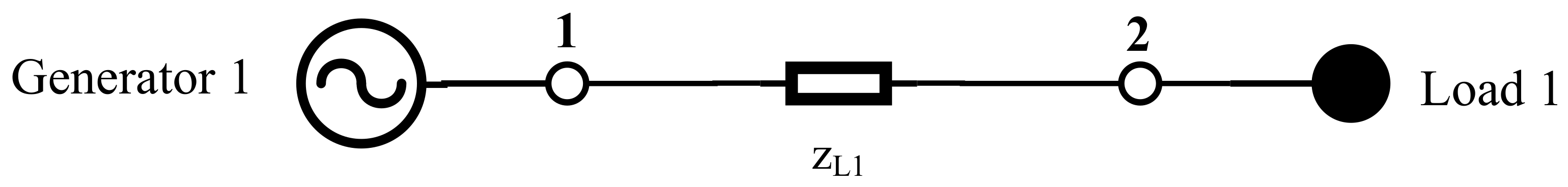
4.1. Representation of a Load as Impedance

In literature, there exist three different models for loads depending on their characteristic (constant power, constant impedance or constant current). In most OPF calculations, only constant power loads are used. In this paper, constant power and constant impedance loads are considered as these are the most common load types in German grids [45]. The total power of a load ${\underline{S}}_{\mathrm{B}}^{\mathrm{t}}$ at bus B can then be divided to a part acting as a constant power load ${\underline{S}}_{\mathrm{B},\mathrm{S}}^{\mathrm{t}}$ and a part as constant impedance load ${\underline{S}}_{\mathrm{B},\mathrm{Z}}^{\mathrm{t}}$.

$${\underline{S}}_{\mathrm{B}}^{\mathrm{t}}={\underline{S}}_{\mathrm{B},\mathrm{S}}^{\mathrm{t}}+{\underline{S}}_{\mathrm{B},\mathrm{Z}}^{\mathrm{t}}$$

(11)

If loads are modelled as constant power loads ${\underline{S}}_{\mathrm{B},\mathrm{S}}^{\mathrm{t}}$, the method presented in Section 7.2 and Section 7.3 is applied. Constant impedance loads ${\underline{S}}_{\mathrm{B},\mathrm{Z}}^{\mathrm{t}}$ are represented by an impedance ${\underline{z}}_{\mathrm{LY}}^{\mathrm{t}}$ that is added between point B-CP and B-N. L is a shortcut for Line and Y is the name of the line. B is the bus where the load is connected. C denotes the conductor where the load is connected C = (1, 2, 3 or N). When equipment can only be connected to Phase 1, 2 or 3, the symbol B-CP is used, where CP = (1, 2 or 3). B-N is the corresponding point to point B-CP on the neutral conductor (see Figure 3). The advantage of this representation is that impedances can be easily incorporated in the admittance matrix $\underline{y}$ [31] and hence the impedance matrix $\underline{z}$.

The input data for the loads have to be processed to calculate the value of the impedance. For the constant impedance approach, it is assumed that the nominal power ${\underline{S}}_{\mathrm{B},\mathrm{Z}}^{\mathrm{t}}$ is consumed at nominal voltage ${\underline{v}}_{\mathrm{Nom}}$. So the impedance is calculated as follows

$${\underline{z}}_{\mathrm{LY}}^{\mathrm{t}}=\frac{{({\underline{v}}_{\mathrm{Nom}})}^2}{{\underline{\mathrm{S}}}_{\mathrm{B},\mathrm{Z}}^{\mathrm{t}}}$$

(12)

As the power ${\underline{\mathrm{S}}}_{\mathrm{B},\mathrm{Z}}^{\mathrm{t}}$ consumed by the load may change in each time step t, the impedance ${\underline{\mathrm{S}}}_{\mathrm{LY}}^{\mathrm{t}}$ is also time-dependent. The impedances calculated here to represent a load are part of the calculation of the impedance matrix $\underline{z}$ (see Section 4.2). As ${\underline{\mathrm{S}}}_{\mathrm{LY}}^{\mathrm{t}}$ is time-dependent, the admittance matrix $\underline{y}$ is equally time-dependent. A corresponding label ${\underline{z}}^{\mathrm{t}}$ or ${\underline{y}}^{\mathrm{t}}$ is not used in this paper, for better clarity and as constant impedance loads are only an optional modelling approach.

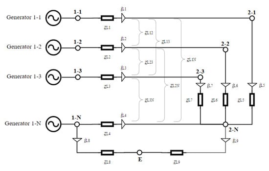
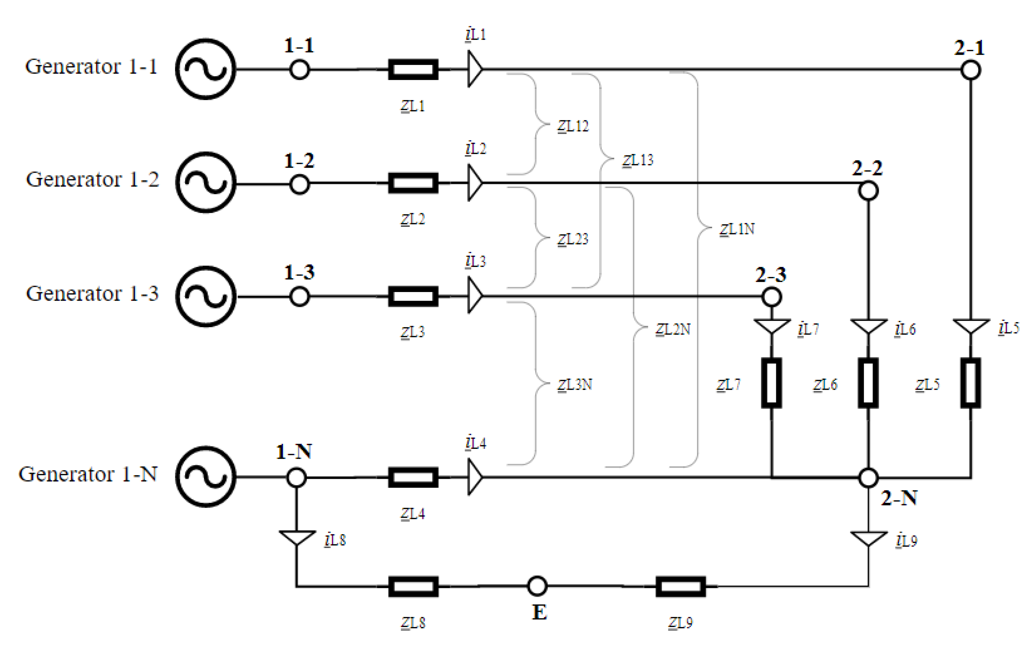
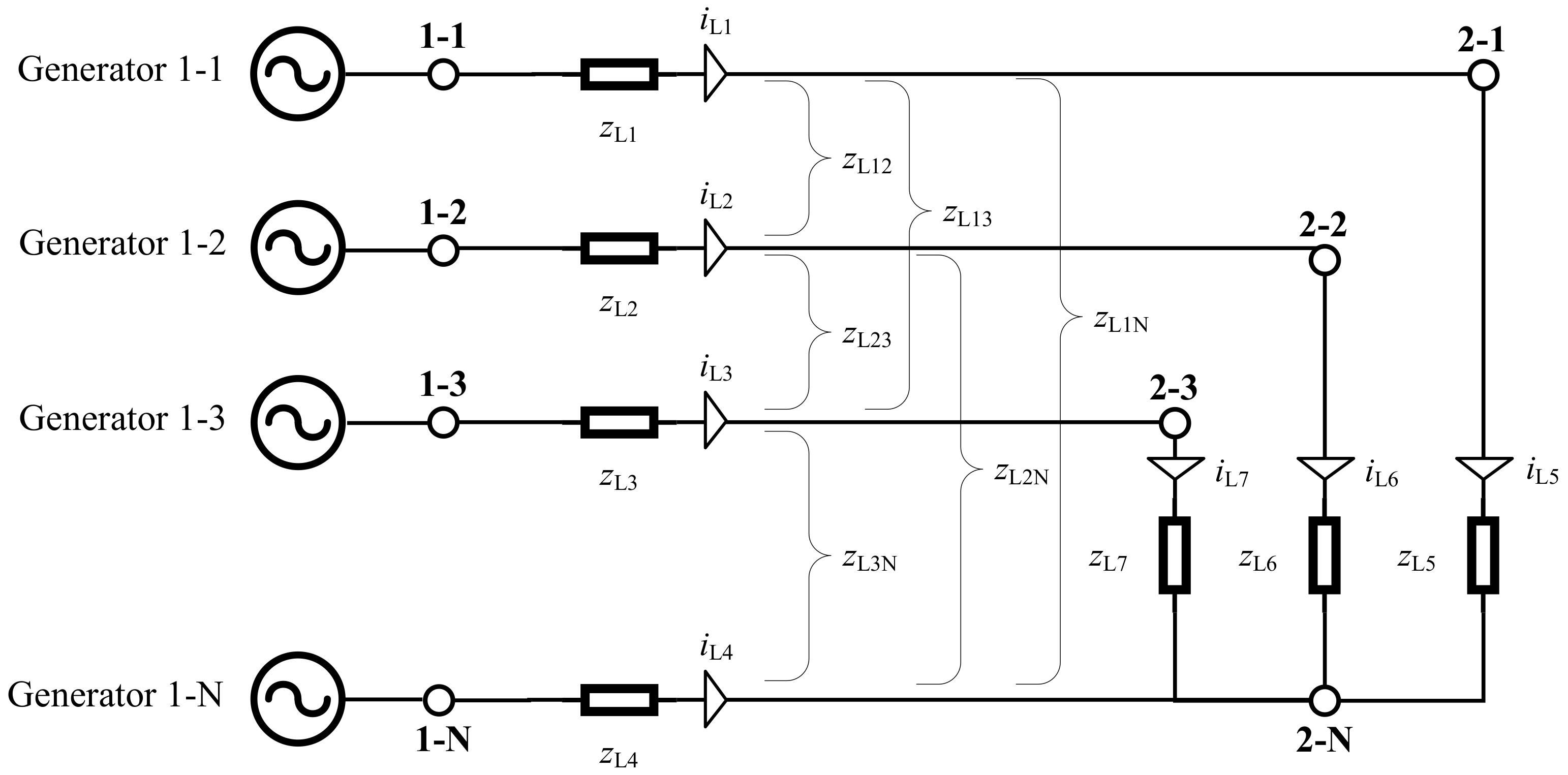
4.2. The Impedance Matrix

The impedance matrix $\underline{z}$ is used to calculate the currents and power flows in the grid depending on the voltages. $\overrightarrow{{\underline{v}}^{\mathrm{t}}}$ is a vector containing all voltages at time step t. A vector with currents flowing on all lines ${\overrightarrow{{\underline{i}}^{\mathrm{t}}}}_{\mathrm{Line}}$ can be calculated as follows:

$${\overrightarrow{{\underline{i}}^{\mathrm{t}}}}_{\mathrm{Line}}={\underline{z}}^{-1}·\overrightarrow{{\underline{v}}^{\mathrm{t}}}=\underline{y}·\overrightarrow{{\underline{v}}^{\mathrm{t}}}$$

(13)

The admittance matrix $\underline{y}$ is the inverse of the impedance matrix $\underline{z}$. For the test grid shown in Figure 3, the impedance matrix $\underline{z}$ is a 7 × 8 matrix having the following form:

$$\left(\begin{array}{c}{\underline{i}}_{\mathrm{L}1}^{\mathrm{t}}\\ {\underline{i}}_{\mathrm{L}2}^{\mathrm{t}}\\ {\underline{i}}_{\mathrm{L}3}^{\mathrm{t}}\\ {\underline{i}}_{\mathrm{L}4}^{\mathrm{t}}\\ {\underline{i}}_{\mathrm{L}5}^{\mathrm{t}}\\ {\underline{i}}_{\mathrm{L}6}^{\mathrm{t}}\\ {\underline{i}}_{\mathrm{L}7}^{\mathrm{t}}\end{array}\right)={\left(\begin{array}{cccccccc}{\underline{z}}_{11}& {\underline{z}}_{12}& {\underline{z}}_{13}& {\underline{z}}_{14}& {\underline{z}}_{15}& {\underline{z}}_{16}& {\underline{z}}_{17}& {\underline{z}}_{18}\\ {\underline{z}}_{21}& {\underline{z}}_{22}& {\underline{z}}_{23}& {\underline{z}}_{24}& {\underline{z}}_{25}& {\underline{z}}_{26}& {\underline{z}}_{27}& {\underline{z}}_{28}\\ {\underline{z}}_{31}& {\underline{z}}_{32}& {\underline{z}}_{33}& {\underline{z}}_{34}& {\underline{z}}_{35}& {\underline{z}}_{36}& {\underline{z}}_{37}& {\underline{z}}_{38}\\ {\underline{z}}_{41}& {\underline{z}}_{42}& {\underline{z}}_{43}& {\underline{z}}_{44}& {\underline{z}}_{45}& {\underline{z}}_{46}& {\underline{z}}_{47}& {\underline{z}}_{48}\\ {\underline{z}}_{51}& {\underline{z}}_{52}& {\underline{z}}_{53}& {\underline{z}}_{54}& {\underline{z}}_{55}& {\underline{z}}_{56}& {\underline{z}}_{57}& {\underline{z}}_{58}\\ {\underline{z}}_{61}& {\underline{z}}_{62}& {\underline{z}}_{63}& {\underline{z}}_{64}& {\underline{z}}_{65}& {\underline{z}}_{66}& {\underline{z}}_{67}& {\underline{z}}_{68}\\ {\underline{z}}_{71}& {\underline{z}}_{72}& {\underline{z}}_{73}& {\underline{z}}_{74}& {\underline{z}}_{75}& {\underline{z}}_{76}& {\underline{z}}_{77}& {\underline{z}}_{78}\end{array}\right)}^{-1}·\left(\begin{array}{c}{\underline{v}}_{1\text{-}1}^{\mathrm{t}}\\ {\underline{v}}_{2\text{-}1}^{\mathrm{t}}\\ {\underline{v}}_{1\text{-}2}^{\mathrm{t}}\\ {\underline{v}}_{2\text{-}2}^{\mathrm{t}}\\ {\underline{v}}_{1\text{-}3}^{\mathrm{t}}\\ {\underline{v}}_{2\text{-}3}^{\mathrm{t}}\\ {\underline{v}}_{1\text{-}\mathrm{N}}^{\mathrm{t}}\\ {\underline{v}}_{2\text{-}\mathrm{N}}^{\mathrm{t}}\end{array}\right)$$

(14)

The naming is in accordance to Figure 3. ${\underline{v}}_{\mathrm{B}\text{-}\mathrm{C}}^{\mathrm{t}}$ refers to the complex voltage at point B-C. In Equation (15), the current on Line 1 ${\underline{i}}_{\mathrm{L}1}^{\mathrm{t}}$ is calculated as an example for the grid in Figure 3.

$${\underline{i}}_{\mathrm{L}1}^{\mathrm{t}}=\frac{1}{{\underline{z}}_{\mathrm{L}1}}·{\underline{v}}_{1,1}^{\mathrm{t}}-\frac{1}{{\underline{z}}_{\mathrm{L}1}}·{\underline{v}}_{2,1}^{\mathrm{t}}=\frac{{\underline{v}}_{1,1}^{\mathrm{t}}-{\underline{v}}^{\mathrm{t}}{}_{2,1}}{{\underline{z}}_{\mathrm{L}1}}$$

(15)

For the test grid shown in Figure 3, the impedance matrix $\underline{z}$ has the following entries:

$$\left(\begin{array}{c}{\underline{i}}_{\mathrm{L}1}^{\mathrm{t}}\\ {\underline{i}}_{\mathrm{L}2}^{\mathrm{t}}\\ {\underline{i}}_{\mathrm{L}3}^{\mathrm{t}}\\ {\underline{i}}_{\mathrm{L}4}^{\mathrm{t}}\\ {\underline{i}}_{\mathrm{L}5}^{\mathrm{t}}\\ {\underline{i}}_{\mathrm{L}6}^{\mathrm{t}}\\ {\underline{i}}_{\mathrm{L}7}^{\mathrm{t}}\end{array}\right)={\left(\begin{array}{cccccccc}{\underline{z}}_{\mathrm{L}1}& -{\underline{z}}_{\mathrm{L}1}& 0& 0& 0& 0& 0& 0\\ 0& 0& {\underline{z}}_{\mathrm{L}2}& -{\underline{z}}_{\mathrm{L}2}& 0& 0& 0& 0\\ 0& 0& 0& 0& {\underline{z}}_{\mathrm{L}3}& -{\underline{z}}_{\mathrm{L}3}& 0& 0\\ 0& 0& 0& 0& 0& 0& {\underline{z}}_{\mathrm{L}4}& -{\underline{z}}_{\mathrm{L}4}\\ 0& {\underline{z}}_{\mathrm{L}5}& 0& 0& 0& 0& 0& -{\underline{z}}_{\mathrm{L}5}\\ 0& 0& 0& {\underline{z}}_{\mathrm{L}6}& 0& 0& 0& -{\underline{z}}_{\mathrm{L}6}\\ 0& 0& 0& 0& 0& {\underline{z}}_{\mathrm{L}7}& 0& -{\underline{z}}_{\mathrm{L}7}\end{array}\right)}^{-1}·\left(\begin{array}{c}{\underline{v}}_{1\text{-}1}^{\mathrm{t}}\\ {\underline{v}}_{2\text{-}1}^{\mathrm{t}}\\ {\underline{v}}_{1\text{-}2}^{\mathrm{t}}\\ {\underline{v}}_{2\text{-}2}^{\mathrm{t}}\\ {\underline{v}}_{1\text{-}3}^{\mathrm{t}}\\ {\underline{v}}_{2\text{-}3}^{\mathrm{t}}\\ {\underline{v}}_{1\text{-}\mathrm{N}}^{\mathrm{t}}\\ {\underline{v}}_{2\text{-}\mathrm{N}}^{\mathrm{t}}\end{array}\right)$$

(16)

In real low voltage grids, there are inductive and conductive couplings between the different phases as seen in Figure 4. For a correct calculation, especially for unbalanced power flows, these mutual impedances have to be considered [44].

Taking into account the mutual impedances leads to the following impedance matrix $\underline{z}$:

$$\underline{z}=\left(\begin{array}{cccccccc}{\underline{z}}_{\mathrm{L}1}& -{\underline{z}}_{\mathrm{L}1}& {\underline{z}}_{\mathrm{L}12}& -{\underline{z}}_{\mathrm{L}12}& {\underline{z}}_{\mathrm{L}13}& -{\underline{z}}_{\mathrm{L}13}& {\underline{z}}_{\mathrm{L}1\mathrm{N}}& -{\underline{z}}_{\mathrm{L}1\mathrm{N}}\\ {\underline{z}}_{\mathrm{L}21}& -{\underline{z}}_{\mathrm{L}21}& {\underline{z}}_{\mathrm{L}2}& -{\underline{z}}_{\mathrm{L}2}& {\underline{z}}_{\mathrm{L}23}& -{\underline{z}}_{\mathrm{L}23}& {\underline{z}}_{\mathrm{L}2\mathrm{N}}& -{\underline{z}}_{\mathrm{L}2\mathrm{N}}\\ {\underline{z}}_{\mathrm{L}31}& -{\underline{z}}_{\mathrm{L}31}& {\underline{z}}_{\mathrm{L}32}& -{\underline{z}}_{\mathrm{L}32}& {\underline{z}}_{\mathrm{L}3}& -{\underline{z}}_{\mathrm{L}3}& {\underline{z}}_{\mathrm{L}3\mathrm{N}}& -{\underline{z}}_{\mathrm{L}3\mathrm{N}}\\ {\underline{z}}_{\mathrm{L}\mathrm{N}1}& -{\underline{z}}_{\mathrm{L}\mathrm{N}1}& {\underline{z}}_{\mathrm{L}\mathrm{N}2}& -{\underline{z}}_{\mathrm{L}\mathrm{N}2}& {\underline{z}}_{\mathrm{L}\mathrm{N}3}& -{\underline{z}}_{\mathrm{L}\mathrm{N}3}& {\underline{z}}_4& -{\underline{z}}_4\\ 0& {\underline{z}}_{\mathrm{L}5}& 0& 0& 0& 0& 0& -{\underline{z}}_{\mathrm{L}5}\\ 0& 0& 0& {\underline{z}}_{\mathrm{L}6}& 0& 0& 0& -{\underline{z}}_{\mathrm{L}6}\\ 0& 0& 0& 0& 0& {\underline{z}}_{\mathrm{L}7}& 0& -{\underline{z}}_{\mathrm{L}7}\end{array}\right)$$

(17)

Under normal circumstances, the impedances of a line ${\underline{z}}_{\mathrm{L}1}$, ${\underline{z}}_{\mathrm{L}2}$ and ${\underline{z}}_{\mathrm{L}3}$ are equal. Therefore, ${\underline{z}}_{\mathrm{S}}$ is introduced as series impedance of the cable.

$${\underline{z}}_{\mathrm{S}}={\underline{z}}_{\mathrm{L}1}={\underline{z}}_{\mathrm{L}2}={\underline{z}}_{\mathrm{L}3}={\underline{z}}_{\mathrm{L}4}$$

(18)

The mutual impedances are not the same as the distances between the different conductors inside the cable are not the same. As can be seen in [44], the assumption of same impedances leads only to minor differences in the results, therefore the mean value of the mutual impedance ${\underline{z}}_{\mathrm{M}}$ is used for all mutual impedances in this paper.

$${\underline{z}}_{\mathrm{M}}={\underline{z}}_{\mathrm{L}12}={\underline{z}}_{\mathrm{L}13}={\underline{z}}_{\mathrm{L}1\mathrm{N}}={\underline{z}}_{\mathrm{L}21}={\underline{z}}_{\mathrm{L}23}={\underline{z}}_{\mathrm{L}2\mathrm{N}}={\underline{z}}_{\mathrm{L}31}={\underline{z}}_{\mathrm{L}32}={\underline{z}}_{\mathrm{L}3\mathrm{N}}$$

(19)

$$={\underline{z}}_{\mathrm{L}\mathrm{N}1}={\underline{z}}_{\mathrm{L}\mathrm{N}2}={\underline{z}}_{\mathrm{L}\mathrm{N}3}$$

Using the newly introduced variables ${\underline{z}}_{\mathrm{S}}$ and ${\underline{z}}_{\mathrm{M}}$, the set of equations in Equation (17) can be simplified to Equation (20).

$$\left(\begin{array}{c}{\underline{i}}_{\mathrm{L}1}^{\mathrm{t}}\\ {\underline{i}}_{\mathrm{L}2}^{\mathrm{t}}\\ {\underline{i}}_{\mathrm{L}3}^{\mathrm{t}}\\ {\underline{i}}_{\mathrm{L}4}^{\mathrm{t}}\\ {\underline{i}}_{\mathrm{L}5}^{\mathrm{t}}\\ {\underline{i}}_{\mathrm{L}6}^{\mathrm{t}}\\ {\underline{i}}_{\mathrm{L}7}^{\mathrm{t}}\end{array}\right)={\left(\begin{array}{cccccccc}{\underline{z}}_{\mathrm{S}}& -{\underline{z}}_{\mathrm{S}}& {\underline{z}}_{\mathrm{M}}& -{\underline{z}}_{\mathrm{M}}& {\underline{z}}_{\mathrm{M}}& -{\underline{z}}_{\mathrm{M}}& {\underline{z}}_{\mathrm{M}}& -{\underline{z}}_{\mathrm{M}}\\ {\underline{z}}_{\mathrm{M}}& -{\underline{z}}_{\mathrm{M}}& {\underline{z}}_{\mathrm{S}}& -{\underline{z}}_{\mathrm{S}}& {\underline{z}}_{\mathrm{M}}& -{\underline{z}}_{\mathrm{M}}& {\underline{z}}_{\mathrm{M}}& -{\underline{z}}_{\mathrm{M}}\\ {\underline{z}}_{\mathrm{M}}& -{\underline{z}}_{\mathrm{M}}& {\underline{z}}_{\mathrm{M}}& -{\underline{z}}_{\mathrm{M}}& {\underline{z}}_{\mathrm{S}}& -{\underline{z}}_{\mathrm{S}}& {\underline{z}}_{\mathrm{M}}& -{\underline{z}}_{\mathrm{M}}\\ {\underline{z}}_{\mathrm{M}}& -{\underline{z}}_{\mathrm{M}}& {\underline{z}}_{\mathrm{M}}& -{\underline{z}}_{\mathrm{M}}& {\underline{z}}_{\mathrm{M}}& -{\underline{z}}_{\mathrm{M}}& {\underline{z}}_{\mathrm{S}}& -{\underline{z}}_{\mathrm{S}}\\ 0& {\underline{z}}_{\mathrm{L}5}& 0& 0& 0& 0& 0& -{\underline{z}}_{\mathrm{L}5}\\ 0& 0& 0& {\underline{z}}_{\mathrm{L}6}& 0& 0& 0& -{\underline{z}}_{\mathrm{L}6}\\ 0& 0& 0& 0& 0& {\underline{z}}_{\mathrm{L}7}& 0& -{\underline{z}}_{\mathrm{L}7}\end{array}\right)}^{-1}·\left(\begin{array}{c}{\underline{v}}_{1\text{-}1}^{\mathrm{t}}\\ {\underline{v}}_{2\text{-}1}^{\mathrm{t}}\\ {\underline{v}}_{1\text{-}2}^{\mathrm{t}}\\ {\underline{v}}_{2\text{-}2}^{\mathrm{t}}\\ {\underline{v}}_{1\text{-}3}^{\mathrm{t}}\\ {\underline{v}}_{2\text{-}3}^{\mathrm{t}}\\ {\underline{v}}_{1\text{-}\mathrm{N}}^{\mathrm{t}}\\ {\underline{v}}_{2\text{-}\mathrm{N}}^{\mathrm{t}}\end{array}\right)$$

(20)

In Germany, there are several grounding points in a low voltage grid. Besides a grounding point at the low voltage side of the MV/LV transformer, there are additional connections to earth at each household as well as at cable distribution cabinets. Hence, an additional conductive path exists through earth. As shown in [44], neglecting this conductive path leads to significant deviations. To model the conductive path through earth, an approach presented in [44] is used. It consists of an imaginary point that represents the earth. This point is named E in Figure 5.

All points in the low voltage grid being grounded are connected to this point directly via an earthing resistance. This earthing resistance consists of the contact resistance between earthing device and ground as well as the resistance of the ground. In

Table 1. Earthing resistances from [44].

Equipment	Earthing Resistance
Transformer	6 $\Omega$
Household	2 $\Omega$
Cable distribution cabinet	2 $\Omega$

, the values of the assumed earthing resistances according to [44] are shown.

As the points 1-1, 1-2, 1-3 and 1-N in Figure 4 model the low voltage side of a MV/LV transformer and the points 2-1, 2-2, 2-3 and 2-N for example a load in a household, the resulting grid model including grounding points can be seen in Figure 5. The corresponding impedance matrix $\underline{z}$ is then a 9 × 9 matrix as shown in Equation (21).

$$\left(\begin{array}{c}{\underline{i}}_{\mathrm{L}1}^{\mathrm{t}}\\ {\underline{i}}_{\mathrm{L}2}^{\mathrm{t}}\\ {\underline{i}}_{\mathrm{L}3}^{\mathrm{t}}\\ {\underline{i}}_{\mathrm{L}4}^{\mathrm{t}}\\ {\underline{i}}_{\mathrm{L}5}^{\mathrm{t}}\\ {\underline{i}}_{\mathrm{L}6}^{\mathrm{t}}\\ {\underline{i}}_{\mathrm{L}7}^{\mathrm{t}}\\ {\underline{i}}_{\mathrm{L}8}^{\mathrm{t}}\\ {\underline{i}}_{\mathrm{L}9}^{\mathrm{t}}\end{array}\right)={\left(\begin{array}{ccccccccc}{\underline{z}}_{\mathrm{S}}& -{\underline{z}}_{\mathrm{S}}& {\underline{z}}_{\mathrm{M}}& -{\underline{z}}_{\mathrm{M}}& {\underline{z}}_{\mathrm{M}}& -{\underline{z}}_{\mathrm{M}}& {\underline{z}}_{\mathrm{M}}& -{\underline{z}}_{\mathrm{M}}& 0\\ {\underline{z}}_{\mathrm{M}}& -{\underline{z}}_{\mathrm{M}}& {\underline{z}}_{\mathrm{S}}& -{\underline{z}}_{\mathrm{S}}& {\underline{z}}_{\mathrm{M}}& -{\underline{z}}_{\mathrm{M}}& {\underline{z}}_{\mathrm{M}}& -{\underline{z}}_{\mathrm{M}}& 0\\ {\underline{z}}_{\mathrm{M}}& -{\underline{z}}_{\mathrm{M}}& {\underline{z}}_{\mathrm{M}}& -{\underline{z}}_{\mathrm{M}}& {\underline{z}}_{\mathrm{S}}& -{\underline{z}}_{\mathrm{S}}& {\underline{z}}_{\mathrm{M}}& -{\underline{z}}_{\mathrm{M}}& 0\\ {\underline{z}}_{\mathrm{M}}& -{\underline{z}}_{\mathrm{M}}& {\underline{z}}_{\mathrm{M}}& -{\underline{z}}_{\mathrm{M}}& {\underline{z}}_{\mathrm{M}}& -{\underline{z}}_{\mathrm{M}}& {\underline{z}}_{\mathrm{S}}& -{\underline{z}}_{\mathrm{S}}& 0\\ 0& {\underline{z}}_{\mathrm{L}5}& 0& 0& 0& 0& 0& -{\underline{z}}_{\mathrm{L}5}& 0\\ 0& 0& 0& {\underline{z}}_{\mathrm{L}6}& 0& 0& 0& -{\underline{z}}_{\mathrm{L}6}& 0\\ 0& 0& 0& 0& 0& {\underline{z}}_{\mathrm{L}7}& 0& -{\underline{z}}_{\mathrm{L}7}& 0\\ 0& 0& 0& 0& 0& 0& {\underline{z}}_{\mathrm{L}8}& 0& -{\underline{z}}_{\mathrm{L}8}\\ 0& 0& 0& 0& 0& 0& 0& {\underline{z}}_{\mathrm{L}9}& -{\underline{z}}_{\mathrm{L}9}\end{array}\right)}^{-1}·\left(\begin{array}{c}{\underline{v}}_{1\text{-}1}^{\mathrm{t}}\\ {\underline{v}}_{2\text{-}1}^{\mathrm{t}}\\ {\underline{v}}_{1\text{-}2}^{\mathrm{t}}\\ {\underline{v}}_{2\text{-}2}^{\mathrm{t}}\\ {\underline{v}}_{1\text{-}3}^{\mathrm{t}}\\ {\underline{v}}_{2\text{-}3}^{\mathrm{t}}\\ {\underline{v}}_{1\text{-}\mathrm{N}}^{\mathrm{t}}\\ {\underline{v}}_{2\text{-}\mathrm{N}}^{\mathrm{t}}\\ {\underline{v}}_{\mathrm{E}}^{\mathrm{t}}\end{array}\right)$$

(21)

4.3. The Nodal Impedance Matrix

The nodal impedance matrix ${\underline{z}}_{\mathrm{Nodal}}$ is calculated using $\underline{z}$ and is used to calculate the sum of the currents that are flowing from a point B-C to other points. ${\overrightarrow{{\underline{i}}^{\mathrm{t}}}}_{\mathrm{Bus}}$ is a vector containing all these currents while ${\underline{i}}_{\mathrm{B}\text{-}\mathrm{C}}^{\mathrm{t}}$ refers to the sum of the currents at point B-C.

$${\overrightarrow{{\underline{i}}^{\mathrm{t}}}}_{\mathrm{Bus}}={{\underline{z}}_{\mathrm{Nodal}}}^{-1}·\overrightarrow{{\underline{v}}^{\mathrm{t}}}$$

(22)

Consequently, ${\underline{i}}_{B\text{-}\mathrm{C}}^{\mathrm{t}}$ can be calculated using the currents given in Equation (21).

$$\left(\begin{array}{c}{\underline{i}}_{1\text{-}1}^{\mathrm{t}}\\ {\underline{i}}_{2\text{-}1}^{\mathrm{t}}\\ {\underline{i}}_{1\text{-}2}^{\mathrm{t}}\\ {\underline{i}}_{2\text{-}2}^{\mathrm{t}}\\ {\underline{i}}_{1\text{-}3}^{\mathrm{t}}\\ {\underline{i}}_{2\text{-}3}^{\mathrm{t}}\\ {\underline{i}}_{1\text{-}\mathrm{N}}^{\mathrm{t}}\\ {\underline{i}}_{2\text{-}\mathrm{N}}^{\mathrm{t}}\\ {\underline{i}}_{\mathrm{E}}^{\mathrm{t}}\end{array}\right)=\left(\begin{array}{c}{\underline{i}}_{\mathrm{L}1}^{\mathrm{t}}\\ -{\underline{i}}_{\mathrm{L}1}^{\mathrm{t}}+{\underline{i}}_{\mathrm{L}5}^{\mathrm{t}}\\ {\underline{i}}_{\mathrm{L}2}^{\mathrm{t}}\\ -{\underline{i}}_{\mathrm{L}2}^{\mathrm{t}}+{\underline{i}}_{\mathrm{L}6}^{\mathrm{t}}\\ {\underline{i}}_{\mathrm{L}3}^{\mathrm{t}}\\ -{\underline{i}}_{\mathrm{L}3}^{\mathrm{t}}+{\underline{i}}_{\mathrm{L}7}^{\mathrm{t}}\\ {\underline{i}}_{\mathrm{L}4}^{\mathrm{t}}+{\underline{i}}_{\mathrm{L}8}^{\mathrm{t}}\\ -{\underline{i}}_{\mathrm{L}4}^{\mathrm{t}}-{\underline{i}}_{\mathrm{L}5}^{\mathrm{t}}-{\underline{i}}_{\mathrm{L}6}^{\mathrm{t}}-{\underline{i}}_{\mathrm{L}7}^{\mathrm{t}}+{\underline{i}}_{\mathrm{L}9}^{\mathrm{t}}\\ -{\underline{i}}_{\mathrm{L}8}^{\mathrm{t}}-{\underline{i}}_{\mathrm{L}9}^{\mathrm{t}}\end{array}\right)$$

(23)

Assuming, a grid structure like in Figure 5, ${\underline{z}}_{\mathrm{Nodal}}$ is a 9 × 9 matrix.

$${\underline{z}}_{\mathrm{Nodal}}=\left(\begin{array}{ccccccccc}{\underline{z}}_{\mathrm{Nodal},11}& {\underline{z}}_{\mathrm{Nodal},12}& {\underline{z}}_{\mathrm{Nodal},13}& {\underline{z}}_{\mathrm{Nodal},14}& {\underline{z}}_{\mathrm{Nodal},15}& {\underline{z}}_{\mathrm{Nodal},16}& {\underline{z}}_{\mathrm{Nodal},17}& {\underline{z}}_{\mathrm{Nodal},18}& {\underline{z}}_{\mathrm{Nodal},19}\\ {\underline{z}}_{\mathrm{Nodal},21}& {\underline{z}}_{\mathrm{Nodal},22}& {\underline{z}}_{\mathrm{Nodal},23}& {\underline{z}}_{\mathrm{Nodal},24}& {\underline{z}}_{\mathrm{Nodal},25}& {\underline{z}}_{\mathrm{Nodal},26}& {\underline{z}}_{\mathrm{Nodal},27}& {\underline{z}}_{\mathrm{Nodal},28}& {\underline{z}}_{\mathrm{Nodal},29}\\ {\underline{z}}_{\mathrm{Nodal},31}& {\underline{z}}_{\mathrm{Nodal},32}& {\underline{z}}_{\mathrm{Nodal},33}& {\underline{z}}_{\mathrm{Nodal},34}& {\underline{z}}_{\mathrm{Nodal},35}& {\underline{z}}_{\mathrm{Nodal},36}& {\underline{z}}_{\mathrm{Nodal},37}& {\underline{z}}_{\mathrm{Nodal},38}& {\underline{z}}_{\mathrm{Nodal},39}\\ {\underline{z}}_{\mathrm{Nodal},41}& {\underline{z}}_{\mathrm{Nodal},42}& {\underline{z}}_{\mathrm{Nodal},43}& {\underline{z}}_{\mathrm{Nodal},44}& {\underline{z}}_{\mathrm{Nodal},45}& {\underline{z}}_{\mathrm{Nodal},46}& {\underline{z}}_{\mathrm{Nodal},47}& {\underline{z}}_{\mathrm{Nodal},48}& {\underline{z}}_{\mathrm{Nodal},49}\\ {\underline{z}}_{\mathrm{Nodal},51}& {\underline{z}}_{\mathrm{Nodal},52}& {\underline{z}}_{\mathrm{Nodal},53}& {\underline{z}}_{\mathrm{Nodal},54}& {\underline{z}}_{\mathrm{Nodal},55}& {\underline{z}}_{\mathrm{Nodal},56}& {\underline{z}}_{\mathrm{Nodal},57}& {\underline{z}}_{\mathrm{Nodal},58}& {\underline{z}}_{\mathrm{Nodal},59}\\ {\underline{z}}_{\mathrm{Nodal},61}& {\underline{z}}_{\mathrm{Nodal},62}& {\underline{z}}_{\mathrm{Nodal},63}& {\underline{z}}_{\mathrm{Nodal},64}& {\underline{z}}_{\mathrm{Nodal},65}& {\underline{z}}_{\mathrm{Nodal},66}& {\underline{z}}_{\mathrm{Nodal},67}& {\underline{z}}_{\mathrm{Nodal},68}& {\underline{z}}_{\mathrm{Nodal},69}\\ {\underline{z}}_{\mathrm{Nodal},71}& {\underline{z}}_{\mathrm{Nodal},72}& {\underline{z}}_{\mathrm{Nodal},73}& {\underline{z}}_{\mathrm{Nodal},74}& {\underline{z}}_{\mathrm{Nodal},75}& {\underline{z}}_{\mathrm{Nodal},76}& {\underline{z}}_{\mathrm{Nodal},77}& {\underline{z}}_{\mathrm{Nodal},78}& {\underline{z}}_{\mathrm{Nodal},79}\\ {\underline{z}}_{\mathrm{Nodal},81}& {\underline{z}}_{\mathrm{Nodal},82}& {\underline{z}}_{\mathrm{Nodal},83}& {\underline{z}}_{\mathrm{Nodal},84}& {\underline{z}}_{\mathrm{Nodal},85}& {\underline{z}}_{\mathrm{Nodal},86}& {\underline{z}}_{\mathrm{Nodal},87}& {\underline{z}}_{\mathrm{Nodal},88}& {\underline{z}}_{\mathrm{Nodal},89}\\ {\underline{z}}_{\mathrm{Nodal},91}& {\underline{z}}_{\mathrm{Nodal},92}& {\underline{z}}_{\mathrm{Nodal},93}& {\underline{z}}_{\mathrm{Nodal},94}& {\underline{z}}_{\mathrm{Nodal},95}& {\underline{z}}_{\mathrm{Nodal},96}& {\underline{z}}_{\mathrm{Nodal},97}& {\underline{z}}_{\mathrm{Nodal},98}& {\underline{z}}_{\mathrm{Nodal},99}\end{array}\right)$$

(24)

$$=\left(\begin{array}{ccccccccc}{\underline{z}}_{\mathrm{S}}& -{\underline{z}}_{\mathrm{S}}& {\underline{z}}_{\mathrm{M}}& -{\underline{z}}_{\mathrm{M}}& {\underline{z}}_{\mathrm{M}}& -{\underline{z}}_{\mathrm{M}}& {\underline{z}}_{\mathrm{M}}& -{\underline{z}}_{\mathrm{M}}& 0\\ -{\underline{z}}_{\mathrm{S}}& {\underline{z}}_{\mathrm{S}}+{\underline{z}}_{\mathrm{L}5}& -{\underline{z}}_{\mathrm{M}}& {\underline{z}}_{\mathrm{M}}& -{\underline{z}}_{\mathrm{M}}& {\underline{z}}_{\mathrm{M}}& -{\underline{z}}_{\mathrm{M}}& {\underline{z}}_{\mathrm{M}}-{\underline{z}}_{\mathrm{L}5}& 0\\ {\underline{z}}_{\mathrm{M}}& -{\underline{z}}_{\mathrm{M}}& {\underline{z}}_{\mathrm{S}}& -{\underline{z}}_{\mathrm{S}}& {\underline{z}}_{\mathrm{M}}& -{\underline{z}}_{\mathrm{M}}& {\underline{z}}_{\mathrm{M}}& -{\underline{z}}_{\mathrm{M}}& 0\\ -{\underline{z}}_{\mathrm{M}}& {\underline{z}}_{\mathrm{M}}& -{\underline{z}}_{\mathrm{S}}& {\underline{z}}_{\mathrm{S}}+{\underline{z}}_{\mathrm{L}6}& -{\underline{z}}_{\mathrm{M}}& {\underline{z}}_{\mathrm{M}}& -{\underline{z}}_{\mathrm{M}}& {\underline{z}}_{\mathrm{M}}-{\underline{z}}_{\mathrm{L}6}& 0\\ {\underline{z}}_{\mathrm{M}}& -{\underline{z}}_{\mathrm{M}}& {\underline{z}}_{\mathrm{M}}& -{\underline{z}}_{\mathrm{M}}& {\underline{z}}_{\mathrm{S}}& -{\underline{z}}_{\mathrm{S}}& {\underline{z}}_{\mathrm{M}}& -{\underline{z}}_{\mathrm{M}}& 0\\ -{\underline{z}}_{\mathrm{M}}& {\underline{z}}_{\mathrm{M}}& -{\underline{z}}_{\mathrm{M}}& {\underline{z}}_{\mathrm{M}}& -{\underline{z}}_{\mathrm{S}}& {\underline{z}}_{\mathrm{S}}+{\underline{z}}_{\mathrm{L}7}& -{\underline{z}}_{\mathrm{M}}& {\underline{z}}_{\mathrm{M}}-{\underline{z}}_{\mathrm{L}7}& 0\\ {\underline{z}}_{\mathrm{M}}& -{\underline{z}}_{\mathrm{M}}& {\underline{z}}_{\mathrm{M}}& -{\underline{z}}_{\mathrm{M}}& {\underline{z}}_{\mathrm{M}}& -{\underline{z}}_{\mathrm{M}}& {\underline{z}}_{\mathrm{S}}+{\underline{z}}_{\mathrm{L}8}& -{\underline{z}}_{\mathrm{S}}& -{\underline{z}}_{\mathrm{L}8}\\ -{\underline{z}}_{\mathrm{M}}& {\underline{z}}_{\mathrm{M}}-{\underline{z}}_{\mathrm{L}5}& -{\underline{z}}_{\mathrm{M}}& {\underline{z}}_{\mathrm{M}}-{\underline{z}}_{\mathrm{L}6}& -{\underline{z}}_{\mathrm{M}}& {\underline{z}}_{\mathrm{M}}-{\underline{z}}_{\mathrm{L}7}& -{\underline{z}}_{\mathrm{S}}& {\underline{z}}_{\mathrm{Nodal},88}& -{\underline{z}}_{\mathrm{L}9}\\ 0& 0& 0& 0& 0& 0& -{\underline{z}}_{\mathrm{L}8}& -{\underline{z}}_{\mathrm{L}9}& {\underline{z}}_{\mathrm{L}8}+{\underline{z}}_{\mathrm{L}9}\end{array}\right)$$

(25)

$${\underline{z}}_{\mathrm{N}odal,88}={\underline{z}}_{\mathrm{L}5}+{\underline{z}}_{\mathrm{L}6}+{\underline{z}}_{\mathrm{L}7}+{\underline{z}}_{\mathrm{S}}+{\underline{z}}_{\mathrm{L}9}$$

(26)

Each impedance as well as each admittance can be divided to a real part and an imaginary part. In Equation (27), the terms used in this publication for each part of the admittance are introduced. Subsequently, the real and imaginary part will be often regarded separately, because the constraints (see Section 7) have to be formulated consisting only of real numbers.

$$\underline{y}=a+j·b$$

(27)

5. Optimization Variables

All optimization variables for one time step are part of the vector x. The number of optimization variables are determined in the following section for an exemplary grid containing only two buses (see Figure 5) for a single time step.

At first, vector x contains the voltages on all points B-C, where B denotes the bus and C the corresponding phase or neutral. The complex voltage is divided to two parts, the real and imaginary part which are denoted as follows.

$${\underline{v}}_{\mathrm{B}\text{-}\mathrm{C}}^{\mathrm{t}}=e_{\mathrm{B}\text{-}\mathrm{C}}^{\mathrm{t}}+j·f_{\mathrm{B}\text{-}\mathrm{C}}^{\mathrm{t}}$$

(28)

For the exemplary grid, these are 16 variables (2 buses · 4 voltages per bus · 2 parts per voltage). Furthermore, vector x contains the real and imaginary part of the voltage at earth (point E in Figure 5).

Additionally, the active power $P_{\mathrm{G},\mathrm{B}\text{-}\mathrm{C}}^{\mathrm{t}}$ as well as the reactive power $Q_{\mathrm{G},\mathrm{B}\text{-}\mathrm{C}}^{\mathrm{t}}$ of all generators are part of the vector x. G is a shortcut for generator and B-C refers to the point of connection of the generator. As there are four generators, there are in total 8 optimization variables.

To include battery storage system, the energy capacity $E_{\mathrm{S},\mathrm{B}}^{\mathrm{t}}$ of the system is another variable in the vector x. S is here a shortcut for storage and B is the bus where the storage is connected. Besides, the active charging $P_{\mathrm{S},\mathrm{C},\mathrm{B}\text{-}\mathrm{CP}}^{\mathrm{t}}$, active discharging power $P_{\mathrm{S},\mathrm{D},\mathrm{B}\text{-}\mathrm{CP}}^{\mathrm{t}}$ and reactive power $Q_{\mathrm{S},\mathrm{B}\text{-}\mathrm{CP}}^{\mathrm{t}}$ needs to be considered. Depending on the design of the battery system, it can be connected to different phases CP at the same bus B. Including one battery system that is connected to all three phases leads to 10 optimization variables.

In total, optimization vector x contains 26 variables without and 36 variables including the battery system. In comparison, the optimization vector x would contain 6 variables without and 10 variables including the battery system for a traditional balanced power flow formulation (see Figure 1).

6. Cost Function

For the cost function, costs are taken into account using cost factors c. These factors are multiplied with a corresponding power and the duration of one time step. In Equation (29), an example is shown where the energy of the generators is priced.

$$F^{\mathrm{t}}=(c_1{P}_{\mathrm{G},1-1}^{\mathrm{t}}+c_2{P}_{\mathrm{G},1-2}^{\mathrm{t}}+c_3{P}_{\mathrm{G},1-3}^{\mathrm{t}}+c_4{P}_{\mathrm{G},1-\mathrm{N}}^{\mathrm{t}})·\Delta t$$

(29)

The cost function in Equation (29) is used in the following simulations. The cost factors of the generator connected to one of the three phases are set to the same value. This value has to be higher than zero to represent the generation costs, so that no unnecessary energy consumption in the low voltage feeder is encouraged. In this paper, it is set to 28 to represent average energy consumption costs in Germany of 28 ct/kWh.

$$c_1=c_2=c_3=28$$

(30)

On the neutral conductor, the current is only flowing back so that no extra costs are assumed.

$$c_4=0$$

(31)

Depending on the optimization goal, the power flow over specific lines or other equipment like a battery storage can be considered additionally.

7. Constraints for the Formulation of the Optimization Problem

In this chapter, the equality and inequality constraints are described. The solver requires the first and second order derivatives of the constraints to solve the optimization problem. For constraints that have already been introduced in literature (e.g., the power flow constraint in Section 7.2), these derivatives are neither given nor mentioned in this section. Only the constraints are explained to the reader.

7.1. Voltage at the Slack Bus

It is necessary to fix the voltage at one point in the regarded grid. For a low voltage feeder, the low voltage side of the MV/LV transformer is chosen. This point is also the slack bus for a low voltage feeder. For the grid in Figure 5, bus 1 is the slack bus.

The magnitude of all voltages at the slack bus is set to 1 p.u. using linear equality constraints. In a three-phase system, there is a 120 degree phase shift between the phases. This phase shift is fixed at the slack bus here to model the feed-in from the medium voltage grid.

$$g_{\mathrm{VSlack}1}^{\mathrm{t}}=e_{1\text{-}1}^{\mathrm{t}}-1=0$$

(32)

$$g_{\mathrm{VSlack}2}^{\mathrm{t}}=f_{1\text{-}1}^{\mathrm{t}}=0$$

(33)

$$g_{\mathrm{VSlack}3}^{\mathrm{t}}=e_{1\text{-}2}^{\mathrm{t}}+0.5=0$$

(34)

$$g_{\mathrm{VSlack}4}^{\mathrm{t}}=f_{1\text{-}2}^{\mathrm{t}}+\frac{\sqrt{3}}{2}=0$$

(35)

$$g_{\mathrm{VSlack}5}^{\mathrm{t}}=e_{1\text{-}3}^{\mathrm{t}}+0.5=0$$

(36)

$$g_{\mathrm{VSlack}6}^{\mathrm{t}}=f_{1\text{-}3}^{\mathrm{t}}-\frac{\sqrt{3}}{2}=0$$

(37)

Additionally, the magnitude and phase of the voltage at the slack bus on the neutral conductor is set to zero.

$$g_{\mathrm{VSlack}7}^{\mathrm{t}}=e_{1\text{-}\mathrm{N}}^{\mathrm{t}}=0$$

(38)

$$g_{\mathrm{VSlack}8}^{\mathrm{t}}=f_{1\text{-}\mathrm{N}}^{\mathrm{t}}=0$$

(39)

As this constraint is a linear constraint, the deviations are all constant.

7.2. Power Flow Equation

At each point in the grid, the power flowing into the point from lines as well as the power generated or consumed at these points have to be balanced. This is taken into account using the following constraints like in [40].

$${\overrightarrow{g^{\mathrm{t}}}}_P={\overrightarrow{P^{\mathrm{t}}}}_{\mathrm{Gen}}-{\overrightarrow{P^{\mathrm{t}}}}_{\mathrm{Bus}}=0$$

(40)

$${\overrightarrow{g^{\mathrm{t}}}}_Q={\overrightarrow{Q^{\mathrm{t}}}}_{\mathrm{Gen}}-{\overrightarrow{Q^{\mathrm{t}}}}_{\mathrm{Bus}}=0$$

(41)

${\overrightarrow{P^{\mathrm{t}}}}_{\mathrm{Gen}}$ is thereby a vector containing the sum of the active power generated by generators, storage systems or constant power loads at all points in the grid. ${\overrightarrow{P^{\mathrm{t}}}}_{\mathrm{Bus}}$ is a vector containing the sum of the active power flowing from one point to other points. ${\overrightarrow{Q^{\mathrm{t}}}}_{\mathrm{Gen}}$ and ${\overrightarrow{Q^{\mathrm{t}}}}_{\mathrm{Bus}}$ are defined accordingly.

${\overrightarrow{P^{\mathrm{t}}}}_{\mathrm{Bus}}$ (Equation (43)) and ${\overrightarrow{Q^{\mathrm{t}}}}_{\mathrm{Bus}}$ (Equation (44)) are determined using Equation (42), where ∘ denotes point-wise multiplication. The nodal admittance matrix ${\underline{y}}_{\mathrm{Nodal}}$ can be separated into a real part $a_{\mathrm{Nodal}}$ and an imaginary part $b_{\mathrm{Nodal}}$ as denoted in Equation (27). The vector $\overrightarrow{{\underline{v}}^{\mathrm{t}}}$ contains all voltages ${\underline{v}}_{\mathrm{B}\text{-}\mathrm{C}}^{\mathrm{t}}$ for time step t and can be separated in $\overrightarrow{e^{\mathrm{t}}}$ and $\overrightarrow{f^{\mathrm{t}}}$ (see Equation (28)). The vector ${\underline{i}}_{\mathrm{Bus}}^{\mathrm{t}}$ contains all currents ${\underline{i}}_{\mathrm{B}\text{-}\mathrm{C}}^{\mathrm{t}}$ for time step t.

$${\overrightarrow{{\underline{S}}^{\mathrm{t}}}}_{\mathrm{Bus}}=\overrightarrow{{\underline{v}}^{\mathrm{t}}}\circ {\overrightarrow{{\underline{i}}^{\mathrm{t}}*}}_{\mathrm{Bus}}=\overrightarrow{{\underline{v}}^{\mathrm{t}}}\circ [{\underline{y}}_{\mathrm{Nodal}}^{*}·\overrightarrow{{\underline{v}}^{\mathrm{t}}*}]$$

(42)

$$=(\overrightarrow{e^{\mathrm{t}}}+j·\overrightarrow{f^{\mathrm{t}}})\circ [(a_{\mathrm{Nodal}}-j·b_{\mathrm{Nodal}})·(\overrightarrow{e^{\mathrm{t}}}-j·\overrightarrow{f^{\mathrm{t}}})]$$

$$=\overrightarrow{e^{\mathrm{t}}}\circ (a_{\mathrm{Nodal}}\overrightarrow{e^{\mathrm{t}}}-b_{\mathrm{Nodal}}\overrightarrow{f^{\mathrm{t}}})+\overrightarrow{f^{\mathrm{t}}}\circ (b_{\mathrm{Nodal}}\overrightarrow{e^{\mathrm{t}}}+a_{\mathrm{Nodal}}\overrightarrow{f^{\mathrm{t}}})$$

$$+j[-\overrightarrow{e^{\mathrm{t}}}\circ (b_{\mathrm{Nodal}}\overrightarrow{e^{\mathrm{t}}}+a_{\mathrm{Nodal}}\overrightarrow{f^{\mathrm{t}}})+\overrightarrow{f^{\mathrm{t}}}\circ (a_{\mathrm{Nodal}}\overrightarrow{e^{\mathrm{t}}}-b_{\mathrm{Nodal}}\overrightarrow{f^{\mathrm{t}}})]$$

$${\overrightarrow{{\mathrm{P}}^{\mathrm{t}}}}_{\mathrm{Bus}}=\overrightarrow{e^{\mathrm{t}}}\circ (a_{\mathrm{Nodal}}\overrightarrow{e^{\mathrm{t}}}-b_{\mathrm{Nodal}}\overrightarrow{f^{\mathrm{t}}})+\overrightarrow{f^{\mathrm{t}}}\circ (b_{\mathrm{Nodal}}\overrightarrow{e^{\mathrm{t}}}+a_{\mathrm{Nodal}}\overrightarrow{f^{\mathrm{t}}})$$

(43)

$${\overrightarrow{Q^{\mathrm{t}}}}_{\mathrm{Bus}}=-\overrightarrow{e^{\mathrm{t}}}\circ (b_{\mathrm{Nodal}}\overrightarrow{e^{\mathrm{t}}}+a_{\mathrm{Nodal}}\overrightarrow{f^{\mathrm{t}}})+\overrightarrow{f^{\mathrm{t}}}\circ (a_{\mathrm{Nodal}}\overrightarrow{e^{\mathrm{t}}}-b_{\mathrm{Nodal}}\overrightarrow{f^{\mathrm{t}}})$$

(44)

7.3. Current Equation

Besides a formulation like in Equations (40) and (41) using power flows, the currents flowing into each point can also be used to formulate an equality constraint. This was introduced in TOPF in [14,17].

$${\overrightarrow{{\underline{i}}^{\mathrm{t}}}}_{\mathrm{Bus}}={\underline{y}}_{\mathrm{Nodal}}·\overrightarrow{{\underline{v}}^{\mathrm{t}}}=(a_{\mathrm{Nodal}}+j·b_{\mathrm{Nodal}})(\overrightarrow{e^{\mathrm{t}}}+j·\overrightarrow{f^{\mathrm{t}}})$$

(45)

$$=a_{\mathrm{Nodal}}·\overrightarrow{e^{\mathrm{t}}}-b_{\mathrm{Nodal}}·\overrightarrow{f^{\mathrm{t}}}+j(b_{\mathrm{Nodal}}·\overrightarrow{e^{\mathrm{t}}}+a_{\mathrm{Nodal}}·\overrightarrow{f^{\mathrm{t}}})$$

The disadvantage of this approach is that power generated or consumed at the concerned bus (see ${\overrightarrow{P^{\mathrm{t}}}}_{\mathrm{Gen}}$ and ${\overrightarrow{Q^{\mathrm{t}}}}_{\mathrm{Gen}}$ in Equations (40) and (41)) can not be considered. Hence, current based equality constraints are only used on points where ${\overrightarrow{P^{\mathrm{t}}}}_{\mathrm{Gen}}$ and ${\overrightarrow{Q^{\mathrm{t}}}}_{\mathrm{Gen}}$ are zero. On the neutral conductor, the power flow is significantly lower than on the other phases. Assuming similar absolute errors in the fulfillment of power flow based equality constraints (see Section 7.2), the relative error is significantly higher on the neutral conductor. Hence, it is beneficial to use current equations on the neutral conductor as currents are in a similar order as on the other phases for unbalanced power flows. Besides a higher accuracy and better conditioned matrices, another advantage is that linear constraints are used instead of nonlinear constraints. The above mentioned disadvantage of this approach is not essential as no power is consumed or generated on the neutral conductor. The only exception is the slack bus due to the generator. In this publication, the current equation instead of the power flow equation is used for all points on the neutral conductor except the slack bus.

For a formulation as a constraints, Equation (45) has to be divided into two parts: One constraint contains the real part and the second the imaginary part of Equation (45). The related constraints are formulated as follows:

$${\overrightarrow{g^{\mathrm{t}}}}_{\mathrm{i},\mathrm{Real}}=a_{\mathrm{Nodal}}·\overrightarrow{e^{\mathrm{t}}}-b_{\mathrm{Nodal}}·\overrightarrow{f^{\mathrm{t}}}=0$$

(46)

$${\overrightarrow{g^{\mathrm{t}}}}_{\mathrm{i},\mathrm{Imag}}=b_{\mathrm{Nodal}}·\overrightarrow{e^{\mathrm{t}}}+a_{\mathrm{Nodal}}·\overrightarrow{f^{\mathrm{t}}}=0$$

(47)

When generators, storage systems or constant power loads are part of the regarded grid, the total generated power at point B-CP $P_{\mathrm{G},\mathrm{B}\text{-}\mathrm{CP}\mathrm{P}}^{\mathrm{t}}$ and $Q_{\mathrm{G},\mathrm{B}\text{-}\mathrm{CP}\mathrm{P}}^{\mathrm{t}}$ is considered in Equations (40) and (41). As the power flow on the neutral conductor is considered in this paper, the negative value of the current being fed into the grid at point B-CP has to be fed-in at point B-N, where point B-N is the corresponding point to B-CP on the neutral conductor of the same bus. This is ensured by expanding the current equation as explained in the following paragraphs.

The current ${\underline{i}}_{\mathrm{G},\mathrm{B}\text{-}\mathrm{C}\mathrm{P}}^{\mathrm{t}}$ that is inserted at point B-CP can be calculated as follows

$${\underline{i}}_{\mathrm{G},\mathrm{B}\text{-}\mathrm{C}\mathrm{P}}^{\mathrm{t}}={\left(\frac{S_{\mathrm{Bus},\mathrm{B}\text{-}\mathrm{C}\mathrm{P}}^{\mathrm{t}}}{{\underline{v}}_{\mathrm{B}\text{-}\mathrm{C}\mathrm{P}}^{\mathrm{t}}}\right)}^{*}=\left(\frac{P_{\mathrm{Bus},\mathrm{B}\text{-}\mathrm{C}\mathrm{P}}^{\mathrm{t}}-j{Q}_{\mathrm{Bus},\mathrm{B}\text{-}\mathrm{C}\mathrm{P}}^{\mathrm{t}}}{e_{\mathrm{B}\text{-}\mathrm{C}\mathrm{P}}^{\mathrm{t}}-j{f}_{\mathrm{B}\text{-}\mathrm{C}\mathrm{P}}^{\mathrm{t}}}\right)\left(\frac{e_{\mathrm{B}\text{-}\mathrm{C}\mathrm{P}}^{\mathrm{t}}+j{f}_{\mathrm{B}\text{-}\mathrm{C}\mathrm{P}}^{\mathrm{t}}}{e_{\mathrm{B}\text{-}\mathrm{C}\mathrm{P}}^{\mathrm{t}}+j{f}_{\mathrm{B}\text{-}\mathrm{C}\mathrm{P}}^{\mathrm{t}}}\right)$$

(48)

$$=\frac{P_{\mathrm{Bus},\mathrm{B}\text{-}\mathrm{C}\mathrm{P}}^{\mathrm{t}}{e}_{\mathrm{B}\text{-}\mathrm{C}\mathrm{P}}^{\mathrm{t}}+Q_{\mathrm{Bus},\mathrm{B}\text{-}\mathrm{C}\mathrm{P}}^{\mathrm{t}}{f}_{\mathrm{B}\text{-}\mathrm{C}\mathrm{P}}^{\mathrm{t}}+j(P_{\mathrm{Bus},\mathrm{B}\text{-}\mathrm{C}\mathrm{P}}^{\mathrm{t}}{f}_{\mathrm{B}\text{-}\mathrm{C}\mathrm{P}}^{\mathrm{t}}-Q_{\mathrm{Bus},\mathrm{B}\text{-}\mathrm{C}\mathrm{P}}^{\mathrm{t}}{e}_{\mathrm{B}\text{-}\mathrm{C}\mathrm{P}}^{\mathrm{t}})}{{(e_{\mathrm{B}\text{-}\mathrm{C}\mathrm{P}}^{\mathrm{t}})}^2+{(f_{\mathrm{B}\text{-}\mathrm{C}\mathrm{P}}^{\mathrm{t}})}^2}$$

$$i_{\mathrm{G},\mathrm{B}\text{-}\mathrm{C}\mathrm{P},\mathrm{Real}}^{\mathrm{t}}=\frac{P_{\mathrm{Bus},\mathrm{B}\text{-}\mathrm{C}\mathrm{P}}^{\mathrm{t}}{e}_{\mathrm{B}\text{-}\mathrm{C}\mathrm{P}}^{\mathrm{t}}+Q_{\mathrm{Bus},\mathrm{B}\text{-}\mathrm{C}\mathrm{P}}^{\mathrm{t}}{f}_{\mathrm{B}\text{-}\mathrm{C}\mathrm{P}}^{\mathrm{t}}}{{(e_{\mathrm{B}\text{-}\mathrm{C}\mathrm{P}}^{\mathrm{t}})}^2+{(f_{\mathrm{B}\text{-}\mathrm{C}\mathrm{P}}^{\mathrm{t}})}^2}$$

(49)

$$i_{\mathrm{G},\mathrm{B}\text{-}\mathrm{C}\mathrm{P},\mathrm{Imag}}^{\mathrm{t}}=\frac{P_{\mathrm{Bus},\mathrm{B}\text{-}\mathrm{C}\mathrm{P}}^{\mathrm{t}}{f}_{\mathrm{B}\text{-}\mathrm{C}\mathrm{P}}^{\mathrm{t}}-Q_{\mathrm{Bus},\mathrm{B}\text{-}\mathrm{C}\mathrm{P}}^{\mathrm{t}}{e}_{\mathrm{B}\text{-}\mathrm{C}\mathrm{P}}^{\mathrm{t}}}{{(e_{\mathrm{B}\text{-}\mathrm{C}\mathrm{P}}^{\mathrm{t}})}^2+{(f_{\mathrm{B}\text{-}\mathrm{C}\mathrm{P}}^{\mathrm{t}})}^2}$$

(50)

The vectors ${\overrightarrow{i^{\mathrm{t}}}}_{\mathrm{G},\mathrm{Real}}$ and ${\overrightarrow{i^{\mathrm{t}}}}_{\mathrm{G},\mathrm{Imag}}$ contain the real and imaginary part of the current that is inserted at all points.

$${\overrightarrow{i^{\mathrm{t}}}}_{\mathrm{G},\mathrm{Real}}=\frac{{\overrightarrow{P^{\mathrm{t}}}}_{\mathrm{Bus}}\circ \overrightarrow{e^{\mathrm{t}}}+{\overrightarrow{Q^{\mathrm{t}}}}_{\mathrm{Bus}}\circ \overrightarrow{f^{\mathrm{t}}}}{{(\overrightarrow{e^{\mathrm{t}}})}^2+{(\overrightarrow{f^{\mathrm{t}}})}^2}$$

(51)

$${\overrightarrow{i^{\mathrm{t}}}}_{\mathrm{G},\mathrm{Imag}}=\frac{{\overrightarrow{P^{\mathrm{t}}}}_{\mathrm{Bus}}\circ \overrightarrow{f^{\mathrm{t}}}-{\overrightarrow{Q^{\mathrm{t}}}}_{\mathrm{Bus}}\circ \overrightarrow{e^{\mathrm{t}}}}{{(\overrightarrow{e^{\mathrm{t}}})}^2+{(\overrightarrow{f^{\mathrm{t}}})}^2}$$

(52)

The current equations as defined in Equations (46) and (47) are adapted as shown in Equations (53) and (54). Please note that fraction line means pointwise division in Equations (51)–(54).

$${\overrightarrow{g^{\mathrm{t}}}}_{\mathrm{i},\mathrm{Real}}=a_{\mathrm{Nodal}}·\overrightarrow{e^{\mathrm{t}}}-b_{\mathrm{Nodal}}·\overrightarrow{f^{\mathrm{t}}}-(-\mathrm{S}·i_{\mathrm{G},\mathrm{B}\text{-}\mathrm{C}\mathrm{P},\mathrm{Imag}}^{\mathrm{t}})$$

(53)

$$=a_{\mathrm{Nodal}}·\overrightarrow{e^{\mathrm{t}}}-b_{\mathrm{Nodal}}·\overrightarrow{f^{\mathrm{t}}}+S·\frac{{\overrightarrow{P^{\mathrm{t}}}}_{\mathrm{Bus}}\circ \overrightarrow{e^{\mathrm{t}}}+{\overrightarrow{Q^{\mathrm{t}}}}_{\mathrm{Bus}}\circ \overrightarrow{f^{\mathrm{t}}}}{{(\overrightarrow{e^{\mathrm{t}}})}^2+{(\overrightarrow{f^{\mathrm{t}}})}^2}=0$$

$${\overrightarrow{g^{\mathrm{t}}}}_{\mathrm{i},\mathrm{Imag}}=b_{\mathrm{Nodal}}·\overrightarrow{e^{\mathrm{t}}}+a_{\mathrm{Nodal}}·\overrightarrow{f^{\mathrm{t}}}-(-S·{\overrightarrow{i^{\mathrm{t}}}}_{\mathrm{G},\mathrm{Imag}})$$

(54)

$$=b_{\mathrm{Nodal}}·\overrightarrow{e^{\mathrm{t}}}+a_{\mathrm{Nodal}}·\overrightarrow{f^{\mathrm{t}}}+S·\frac{{\overrightarrow{P^{\mathrm{t}}}}_{\mathrm{Bus}}\circ \overrightarrow{f^{\mathrm{t}}}-{\overrightarrow{Q^{\mathrm{t}}}}_{\mathrm{Bus}}\circ \overrightarrow{e^{\mathrm{t}}}}{{(\overrightarrow{e^{\mathrm{t}}})}^2+{(\overrightarrow{f^{\mathrm{t}}})}^2}=0$$

The negative value of the current which is fed into the grid at point B-CP has to be fed-in at point B-N, where point B-N is the corresponding point to B-CP on the same bus on the neutral conductor. The allocation of the current which is fed into the grid at point B-CP to the corresponding current on point B-N on the neutral conductor is done by matrix S.

The first order derivatives of $i_{\mathrm{G},\mathrm{B}\text{-}\mathrm{C}\mathrm{P},\mathrm{Real}}^{\mathrm{t}}$ and $i_{\mathrm{G},\mathrm{B}\text{-}\mathrm{C}\mathrm{P},\mathrm{Imag}}^{\mathrm{t}}$ are given in Equations (55)–(62).

$$\frac{\partial i_{\mathrm{G},\mathrm{B}\text{-}\mathrm{C}\mathrm{P},\mathrm{Real}}^{\mathrm{t}}}{\partial {\mathrm{P}}_{\mathrm{Bus},\mathrm{B}\text{-}\mathrm{C}\mathrm{P}}^{\mathrm{t}}}=\frac{e_{\mathrm{B}\text{-}\mathrm{C}\mathrm{P}}^{\mathrm{t}}}{{(e_{\mathrm{B}\text{-}\mathrm{C}\mathrm{P}}^{\mathrm{t}})}^2+{(f_{\mathrm{B}\text{-}\mathrm{C}\mathrm{P}}^{\mathrm{t}})}^2}$$

(55)

$$\frac{\partial i_{\mathrm{G},\mathrm{B}\text{-}\mathrm{C}\mathrm{P},\mathrm{Real}}^{\mathrm{t}}}{\partial Q_{\mathrm{Bus},\mathrm{B}\text{-}\mathrm{C}\mathrm{P}}^{\mathrm{t}}}=\frac{f_{\mathrm{B}\text{-}\mathrm{C}\mathrm{P}}^{\mathrm{t}}}{{(e_{\mathrm{B}\text{-}\mathrm{C}\mathrm{P}}^{\mathrm{t}})}^2+{(f_{\mathrm{B}\text{-}\mathrm{C}\mathrm{P}}^{\mathrm{t}})}^2}$$

(56)

$$\frac{\partial i_{\mathrm{G},\mathrm{B}\text{-}\mathrm{C}\mathrm{P},\mathrm{Real}}^{\mathrm{t}}}{\partial e_{\mathrm{B}\text{-}\mathrm{C}\mathrm{P}}^{\mathrm{t}}}=\frac{P_{\mathrm{Bus},\mathrm{B}\text{-}\mathrm{C}\mathrm{P}}^{\mathrm{t}}({(e_{\mathrm{B}\text{-}\mathrm{C}\mathrm{P}}^{\mathrm{t}})}^2+{(f_{\mathrm{B}\text{-}\mathrm{C}\mathrm{P}}^{\mathrm{t}})}^2)-(P_{\mathrm{Bus},\mathrm{B}\text{-}\mathrm{C}\mathrm{P}}^{\mathrm{t}}{e}_{\mathrm{B}\text{-}\mathrm{C}\mathrm{P}}^{\mathrm{t}}+Q_{\mathrm{Bus},\mathrm{B}\text{-}\mathrm{C}\mathrm{P}}^{\mathrm{t}}{f}_{\mathrm{B}\text{-}\mathrm{C}\mathrm{P}}^{\mathrm{t}})2e_{\mathrm{B}\text{-}\mathrm{C}\mathrm{P}}^{\mathrm{t}}}{{({(e_{\mathrm{B}\text{-}\mathrm{C}\mathrm{P}}^{\mathrm{t}})}^2+{(f_{\mathrm{B}\text{-}\mathrm{C}\mathrm{P}}^{\mathrm{t}})}^2)}^2}$$

(57)

$$\hspace{1em}\hspace{1em}\hspace{1em}=\frac{-P_{\mathrm{Bus},\mathrm{B}\text{-}\mathrm{C}\mathrm{P}}^{\mathrm{t}}{(e_{\mathrm{B}\text{-}\mathrm{C}\mathrm{P}}^{\mathrm{t}})}^2+P_{\mathrm{Bus},\mathrm{B}\text{-}\mathrm{C}\mathrm{P}}^{\mathrm{t}}{(f_{\mathrm{B}\text{-}\mathrm{C}\mathrm{P}}^{\mathrm{t}})}^2-2Q_{\mathrm{Bus},\mathrm{B}\text{-}\mathrm{C}\mathrm{P}}^{\mathrm{t}}{f}_{\mathrm{B}\text{-}\mathrm{C}\mathrm{P}}^{\mathrm{t}}{e}_{\mathrm{B}\text{-}\mathrm{C}\mathrm{P}}^{\mathrm{t}}}{{({(e_{\mathrm{B}\text{-}\mathrm{C}\mathrm{P}}^{\mathrm{t}})}^2+{(f_{\mathrm{B}\text{-}\mathrm{C}\mathrm{P}}^{\mathrm{t}})}^2)}^2}$$

$$\frac{\partial i_{\mathrm{G},\mathrm{B}\text{-}\mathrm{C}\mathrm{P},\mathrm{Real}}^{\mathrm{t}}}{\partial f_{\mathrm{B}\text{-}\mathrm{C}\mathrm{P}}^{\mathrm{t}}}=\frac{Q_{\mathrm{Bus},\mathrm{B}\text{-}\mathrm{C}\mathrm{P}}^{\mathrm{t}}({(e_{\mathrm{B}\text{-}\mathrm{C}\mathrm{P}}^{\mathrm{t}})}^2+{(f_{\mathrm{B}\text{-}\mathrm{C}\mathrm{P}}^{\mathrm{t}})}^2)-(P_{\mathrm{Bus},\mathrm{B}\text{-}\mathrm{C}\mathrm{P}}^{\mathrm{t}}{e}_{\mathrm{B}\text{-}\mathrm{C}\mathrm{P}}^{\mathrm{t}}+Q_{\mathrm{Bus},\mathrm{B}\text{-}\mathrm{C}\mathrm{P}}^{\mathrm{t}}{f}_{\mathrm{B}\text{-}\mathrm{C}\mathrm{P}}^{\mathrm{t}})2f_{\mathrm{B}\text{-}\mathrm{C}\mathrm{P}}^{\mathrm{t}}}{{({(e_{\mathrm{B}\text{-}\mathrm{C}\mathrm{P}}^{\mathrm{t}})}^2+{(f_{\mathrm{B}\text{-}\mathrm{C}\mathrm{P}}^{\mathrm{t}})}^2)}^2}$$

(58)

$$\hspace{1em}\hspace{1em}\hspace{1em}=\frac{Q_{\mathrm{Bus},\mathrm{B}\text{-}\mathrm{C}\mathrm{P}}^{\mathrm{t}}{(e_{\mathrm{B}\text{-}\mathrm{C}\mathrm{P}}^{\mathrm{t}})}^2-Q_{\mathrm{Bus},\mathrm{B}\text{-}\mathrm{C}\mathrm{P}}^{\mathrm{t}}{(f_{\mathrm{B}\text{-}\mathrm{C}\mathrm{P}}^{\mathrm{t}})}^2-2P_{\mathrm{Bus},\mathrm{B}\text{-}\mathrm{C}\mathrm{P}}^{\mathrm{t}}{f}_{\mathrm{B}\text{-}\mathrm{C}\mathrm{P}}^{\mathrm{t}}{e}_{\mathrm{B}\text{-}\mathrm{C}\mathrm{P}}^{\mathrm{t}}}{{({(e_{\mathrm{B}\text{-}\mathrm{C}\mathrm{P}}^{\mathrm{t}})}^2+{(f_{\mathrm{B}\text{-}\mathrm{C}\mathrm{P}}^{\mathrm{t}})}^2)}^2}$$

$$\frac{\partial i_{\mathrm{G},\mathrm{B}\text{-}\mathrm{C}\mathrm{P},\mathrm{Imag}}^{\mathrm{t}}}{\partial P_{\mathrm{Bus},\mathrm{B}\text{-}\mathrm{C}\mathrm{P}}^{\mathrm{t}}}=\frac{f_{\mathrm{B}\text{-}\mathrm{C}\mathrm{P}}^{\mathrm{t}}}{{(e_{\mathrm{B}\text{-}\mathrm{C}\mathrm{P}}^{\mathrm{t}})}^2+{(f_{\mathrm{B}\text{-}\mathrm{C}\mathrm{P}}^{\mathrm{t}})}^2}$$

(59)

$$\frac{\partial i_{\mathrm{G},\mathrm{B}\text{-}\mathrm{C}\mathrm{P},\mathrm{Imag}}^{\mathrm{t}}}{\partial Q_{\mathrm{Bus},\mathrm{B}\text{-}\mathrm{C}\mathrm{P}}^{\mathrm{t}}}=\frac{-e_{\mathrm{B}\text{-}\mathrm{C}\mathrm{P}}^{\mathrm{t}}}{{(e_{\mathrm{B}\text{-}\mathrm{C}\mathrm{P}}^{\mathrm{t}})}^2+{(f_{\mathrm{B}\text{-}\mathrm{C}\mathrm{P}}^{\mathrm{t}})}^2}$$

(60)

$$\frac{\partial i_{\mathrm{G},\mathrm{B}\text{-}\mathrm{C}\mathrm{P},\mathrm{Imag}}^{\mathrm{t}}}{\partial e_{\mathrm{B}\text{-}\mathrm{C}\mathrm{P}}^{\mathrm{t}}}=\frac{-Q_{\mathrm{Bus},\mathrm{B}\text{-}\mathrm{C}\mathrm{P}}^{\mathrm{t}}({(e_{\mathrm{B}\text{-}\mathrm{C}\mathrm{P}}^{\mathrm{t}})}^2+{(f_{\mathrm{B}\text{-}\mathrm{C}\mathrm{P}}^{\mathrm{t}})}^2)-(P_{\mathrm{Bus},\mathrm{B}\text{-}\mathrm{C}\mathrm{P}}^{\mathrm{t}}{f}_{\mathrm{B}\text{-}\mathrm{C}\mathrm{P}}^{\mathrm{t}}-Q_{\mathrm{Bus},\mathrm{B}\text{-}\mathrm{C}\mathrm{P}}^{\mathrm{t}}{e}_{\mathrm{B}\text{-}\mathrm{C}\mathrm{P}}^{\mathrm{t}})2e_{\mathrm{B}\text{-}\mathrm{C}\mathrm{P}}^{\mathrm{t}}}{{({(e_{\mathrm{B}\text{-}\mathrm{C}\mathrm{P}}^{\mathrm{t}})}^2+{(f_{\mathrm{B}\text{-}\mathrm{C}\mathrm{P}}^{\mathrm{t}})}^2)}^2}$$

(61)

$$\hspace{1em}\hspace{1em}\hspace{1em}=\frac{-Q_{\mathrm{Bus},\mathrm{B}\text{-}\mathrm{C}\mathrm{P}}^{\mathrm{t}}{(f_{\mathrm{B}\text{-}\mathrm{C}\mathrm{P}}^{\mathrm{t}})}^2+Q_{\mathrm{Bus},\mathrm{B}\text{-}\mathrm{C}\mathrm{P}}^{\mathrm{t}}{(e_{\mathrm{B}\text{-}\mathrm{C}\mathrm{P}}^{\mathrm{t}})}^2-2P_{\mathrm{Bus},\mathrm{B}\text{-}\mathrm{C}\mathrm{P}}^{\mathrm{t}}{f}_{\mathrm{B}\text{-}\mathrm{C}\mathrm{P}}^{\mathrm{t}}{e}_{\mathrm{B}\text{-}\mathrm{C}\mathrm{P}}^{\mathrm{t}}}{{({(e_{\mathrm{B}\text{-}\mathrm{C}\mathrm{P}}^{\mathrm{t}})}^2+{(f_{\mathrm{B}\text{-}\mathrm{C}\mathrm{P}}^{\mathrm{t}})}^2)}^2}$$

$$\frac{\partial i_{\mathrm{G},\mathrm{B}\text{-}\mathrm{C}\mathrm{P},\mathrm{Imag}}^{\mathrm{t}}}{\partial f_{\mathrm{B}\text{-}\mathrm{C}\mathrm{P}}^{\mathrm{t}}}=\frac{P_{\mathrm{Bus},\mathrm{B}\text{-}\mathrm{C}\mathrm{P}}^{\mathrm{t}}({(e_{\mathrm{B}\text{-}\mathrm{C}\mathrm{P}}^{\mathrm{t}})}^2+{(f_{\mathrm{B}\text{-}\mathrm{C}\mathrm{P}}^{\mathrm{t}})}^2)-(P_{\mathrm{Bus},\mathrm{B}\text{-}\mathrm{C}\mathrm{P}}^{\mathrm{t}}{f}_{\mathrm{B}\text{-}\mathrm{C}\mathrm{P}}^{\mathrm{t}}-Q_{\mathrm{Bus},\mathrm{B}\text{-}\mathrm{C}\mathrm{P}}^{\mathrm{t}}{e}_{\mathrm{B}\text{-}\mathrm{C}\mathrm{P}}^{\mathrm{t}})2f_{\mathrm{B}\text{-}\mathrm{C}\mathrm{P}}^{\mathrm{t}}}{{({(e_{\mathrm{B}\text{-}\mathrm{C}\mathrm{P}}^{\mathrm{t}})}^2+{(f_{\mathrm{B}\text{-}\mathrm{C}\mathrm{P}}^{\mathrm{t}})}^2)}^2}$$

(62)

$$\hspace{1em}\hspace{1em}\hspace{1em}=\frac{-P_{\mathrm{Bus},\mathrm{B}\text{-}\mathrm{C}\mathrm{P}}^{\mathrm{t}}{(f_{\mathrm{B}\text{-}\mathrm{C}\mathrm{P}}^{\mathrm{t}})}^2+P_{\mathrm{Bus},\mathrm{B}\text{-}\mathrm{C}\mathrm{P}}^{\mathrm{t}}{(e_{\mathrm{B}\text{-}\mathrm{C}\mathrm{P}}^{\mathrm{t}})}^2+2Q_{\mathrm{Bus},\mathrm{B}\text{-}\mathrm{C}\mathrm{P}}^{\mathrm{t}}{f}_{\mathrm{B}\text{-}\mathrm{C}\mathrm{P}}^{\mathrm{t}}{e}_{\mathrm{B}\text{-}\mathrm{C}\mathrm{P}}^{\mathrm{t}}}{{({(e_{\mathrm{B}\text{-}\mathrm{C}\mathrm{P}}^{\mathrm{t}})}^2+{(f_{\mathrm{B}\text{-}\mathrm{C}\mathrm{P}}^{\mathrm{t}})}^2)}^2}$$

All non-zero second derivatives are given from Equations (63)–(86).

$$\frac{{\partial }^2{i}_{\mathrm{G},\mathrm{B}\text{-}\mathrm{C}\mathrm{P},\mathrm{Real}}^{\mathrm{t}}}{\partial P_{\mathrm{Bus},\mathrm{B}\text{-}\mathrm{C}\mathrm{P}}^{\mathrm{t}}\partial e_{\mathrm{B}\text{-}\mathrm{C}\mathrm{P}}^{\mathrm{t}}}=\frac{{(e_{\mathrm{B}\text{-}\mathrm{C}\mathrm{P}}^{\mathrm{t}})}^2+{(f_{\mathrm{B}\text{-}\mathrm{C}\mathrm{P}}^{\mathrm{t}})}^2-e_{\mathrm{B}\text{-}\mathrm{C}\mathrm{P}}^{\mathrm{t}}·2e_{\mathrm{B}\text{-}\mathrm{C}\mathrm{P}}^{\mathrm{t}}}{{({(e_{\mathrm{B}\text{-}\mathrm{C}\mathrm{P}}^{\mathrm{t}})}^2+{(f_{\mathrm{B}\text{-}\mathrm{C}\mathrm{P}}^{\mathrm{t}})}^2)}^2}$$

(63)

$$=\frac{-{(e_{\mathrm{B}\text{-}\mathrm{C}\mathrm{P}}^{\mathrm{t}})}^2+{(f_{\mathrm{B}\text{-}\mathrm{C}\mathrm{P}}^{\mathrm{t}})}^2}{{({(e_{\mathrm{B}\text{-}\mathrm{C}\mathrm{P}}^{\mathrm{t}})}^2+{(f_{\mathrm{B}\text{-}\mathrm{C}\mathrm{P}}^{\mathrm{t}})}^2)}^2}$$

$$\frac{{\partial }^2{i}_{\mathrm{G},\mathrm{B}\text{-}\mathrm{C}\mathrm{P},Real}^{\mathrm{t}}}{\partial P_{\mathrm{Bus},\mathrm{B}\text{-}\mathrm{C}\mathrm{P}}^{\mathrm{t}}\partial f_{\mathrm{B}\text{-}\mathrm{C}\mathrm{P}}^{\mathrm{t}}}=\frac{-2e_{\mathrm{B}\text{-}\mathrm{C}\mathrm{P}}^{\mathrm{t}}·f_{\mathrm{B}\text{-}\mathrm{C}\mathrm{P}}^{\mathrm{t}}}{{({(e_{\mathrm{B}\text{-}\mathrm{C}\mathrm{P}}^{\mathrm{t}})}^2+{(f_{\mathrm{B}\text{-}\mathrm{C}\mathrm{P}}^{\mathrm{t}})}^2)}^2}$$

(64)

$$\frac{{\partial }^2{i}_{\mathrm{G},\mathrm{B}\text{-}\mathrm{C}\mathrm{P},\mathrm{Real}}^{\mathrm{t}}}{\partial Q_{\mathrm{Bus},\mathrm{B}\text{-}\mathrm{C}\mathrm{P}}^{\mathrm{t}}\partial e_{\mathrm{B}\text{-}\mathrm{C}\mathrm{P}}^{\mathrm{t}}}=\frac{-2f_{\mathrm{B}\text{-}\mathrm{C}\mathrm{P}}^{\mathrm{t}}·e_{\mathrm{B}\text{-}\mathrm{C}\mathrm{P}}^{\mathrm{t}}}{{({(e_{\mathrm{B}\text{-}\mathrm{C}\mathrm{P}}^{\mathrm{t}})}^2+{(f_{\mathrm{B}\text{-}\mathrm{C}\mathrm{P}}^{\mathrm{t}})}^2)}^2}$$

(65)

$$\frac{{\partial }^2{i}_{\mathrm{G},\mathrm{B}\text{-}\mathrm{C}\mathrm{P},\mathrm{Real}}^{\mathrm{t}}}{\partial Q_{\mathrm{Bus},\mathrm{B}\text{-}\mathrm{C}\mathrm{P}}^{\mathrm{t}}\partial f_{\mathrm{B}\text{-}\mathrm{C}\mathrm{P}}^{\mathrm{t}}}=\frac{{(e_{\mathrm{B}\text{-}\mathrm{C}\mathrm{P}}^{\mathrm{t}})}^2+{(f_{\mathrm{B}\text{-}\mathrm{C}\mathrm{P}}^{\mathrm{t}})}^2-f_{\mathrm{B}\text{-}\mathrm{C}\mathrm{P}}^{\mathrm{t}}·2f_{\mathrm{B}\text{-}\mathrm{C}\mathrm{P}}^{\mathrm{t}}}{{({(e_{\mathrm{B}\text{-}\mathrm{C}\mathrm{P}}^{\mathrm{t}})}^2+{(f_{\mathrm{B}\text{-}\mathrm{C}\mathrm{P}}^{\mathrm{t}})}^2)}^2}$$

(66)

$$=\frac{{(e_{\mathrm{B}\text{-}\mathrm{C}\mathrm{P}}^{\mathrm{t}})}^2-{(f_{\mathrm{B}\text{-}\mathrm{C}\mathrm{P}}^{\mathrm{t}})}^2}{{({(e_{\mathrm{B}\text{-}\mathrm{C}\mathrm{P}}^{\mathrm{t}})}^2+{(f_{\mathrm{B}\text{-}\mathrm{C}\mathrm{P}}^{\mathrm{t}})}^2)}^2}$$

$$\frac{{\partial }^2{i}_{\mathrm{G},\mathrm{B}\text{-}\mathrm{C}\mathrm{P},\mathrm{Real}}^{\mathrm{t}}}{\partial e_{\mathrm{B}\text{-}\mathrm{C}{\mathrm{P}}^2}^{\mathrm{t}}}=\frac{(-2P_{\mathrm{Bus},\mathrm{B}\text{-}\mathrm{C}\mathrm{P}}^{\mathrm{t}}{e}_{\mathrm{B}\text{-}\mathrm{C}\mathrm{P}}^{\mathrm{t}}\text{-}2Q_{\mathrm{Bus},\mathrm{B}\text{-}\mathrm{C}\mathrm{P}}^{\mathrm{t}}{f}_{\mathrm{B}\text{-}\mathrm{C}\mathrm{P}}^{\mathrm{t}})·({(e_{\mathrm{B}\text{-}\mathrm{C}\mathrm{P}}^{\mathrm{t}})}^2+{(f_{\mathrm{B}\text{-}\mathrm{C}\mathrm{P}}^{\mathrm{t}})}^2)}{{({(e_{\mathrm{B}\text{-}\mathrm{C}\mathrm{P}}^{\mathrm{t}})}^2+{(f_{\mathrm{B}\text{-}\mathrm{C}\mathrm{P}}^{\mathrm{t}})}^2)}^3}$$

(67)

$$-\frac{(-P_{\mathrm{Bus},\mathrm{B}\text{-}\mathrm{C}\mathrm{P}}^{\mathrm{t}}{(e_{\mathrm{B}\text{-}\mathrm{C}\mathrm{P}}^{\mathrm{t}})}^2+P_{\mathrm{Bus},\mathrm{B}\text{-}\mathrm{C}\mathrm{P}}^{\mathrm{t}}{(f_{\mathrm{B}\text{-}\mathrm{C}\mathrm{P}}^{\mathrm{t}})}^2-2Q_{\mathrm{Bus},\mathrm{B}\text{-}\mathrm{C}\mathrm{P}}^{\mathrm{t}}{f}_{\mathrm{B}\text{-}\mathrm{C}\mathrm{P}}^{\mathrm{t}}{e}_{\mathrm{B}\text{-}\mathrm{C}\mathrm{P}}^{\mathrm{t}})·4e_{\mathrm{B}\text{-}\mathrm{C}\mathrm{P}}^{\mathrm{t}}}{{({(e_{\mathrm{B}\text{-}\mathrm{C}\mathrm{P}}^{\mathrm{t}})}^2+{(f_{\mathrm{B}\text{-}\mathrm{C}\mathrm{P}}^{\mathrm{t}})}^2)}^3}$$

$$\frac{{\partial }^2{i}_{\mathrm{G},\mathrm{B}\text{-}\mathrm{C}\mathrm{P},Real}^{\mathrm{t}}}{\partial e_{\mathrm{B}\text{-}\mathrm{C}\mathrm{P}}^{\mathrm{t}}\partial f_{\mathrm{B}\text{-}\mathrm{C}\mathrm{P}}^{\mathrm{t}}}=\frac{(2P_{\mathrm{Bus},\mathrm{B}\text{-}\mathrm{C}\mathrm{P}}^{\mathrm{t}}{f}_{\mathrm{B}\text{-}\mathrm{C}\mathrm{P}}^{\mathrm{t}}-2Q_{\mathrm{Bus},\mathrm{B}\text{-}\mathrm{C}\mathrm{P}}^{\mathrm{t}}{e}_{\mathrm{B}\text{-}\mathrm{C}\mathrm{P}}^{\mathrm{t}})·({(e_{\mathrm{B}\text{-}\mathrm{C}\mathrm{P}}^{\mathrm{t}})}^2+{(f_{\mathrm{B}\text{-}\mathrm{C}\mathrm{P}}^{\mathrm{t}})}^2)}{{({(e_{\mathrm{B}\text{-}\mathrm{C}\mathrm{P}}^{\mathrm{t}})}^2+{(f_{\mathrm{B}\text{-}\mathrm{C}\mathrm{P}}^{\mathrm{t}})}^2)}^3}$$

(68)

$$-\frac{(-P_{\mathrm{Bus},\mathrm{B}\text{-}\mathrm{C}\mathrm{P}}^{\mathrm{t}}{(e_{\mathrm{B}\text{-}\mathrm{C}\mathrm{P}}^{\mathrm{t}})}^2+P_{\mathrm{Bus},\mathrm{B}\text{-}\mathrm{C}\mathrm{P}}^{\mathrm{t}}{(f_{\mathrm{B}\text{-}\mathrm{C}\mathrm{P}}^{\mathrm{t}})}^2-2Q_{\mathrm{Bus},\mathrm{B}\text{-}\mathrm{C}\mathrm{P}}^{\mathrm{t}}{f}_{\mathrm{B}\text{-}\mathrm{C}\mathrm{P}}^{\mathrm{t}}{e}_{\mathrm{B}\text{-}\mathrm{C}\mathrm{P}}^{\mathrm{t}})·4f_{\mathrm{B}\text{-}\mathrm{C}\mathrm{P}}^{\mathrm{t}}}{{({(e_{\mathrm{B}\text{-}\mathrm{C}\mathrm{P}}^{\mathrm{t}})}^2+{(f_{\mathrm{B}\text{-}\mathrm{C}\mathrm{P}}^{\mathrm{t}})}^2)}^3}$$

$$\frac{{\partial }^2{i}_{\mathrm{G},\mathrm{B}\text{-}\mathrm{C}\mathrm{P},\mathrm{Real}}^{\mathrm{t}}}{\partial e_{\mathrm{B}\text{-}\mathrm{C}\mathrm{P}}^{\mathrm{t}}\partial P_{\mathrm{Bus},\mathrm{B}\text{-}\mathrm{C}\mathrm{P}}^{\mathrm{t}}}=\frac{-{(e_{\mathrm{B}\text{-}\mathrm{C}\mathrm{P}}^{\mathrm{t}})}^2+{(f_{\mathrm{B}\text{-}\mathrm{C}\mathrm{P}}^{\mathrm{t}})}^2}{{({(e_{\mathrm{B}\text{-}\mathrm{C}\mathrm{P}}^{\mathrm{t}})}^2+{(f_{\mathrm{B}\text{-}\mathrm{C}\mathrm{P}}^{\mathrm{t}})}^2)}^2}$$

(69)

$$\frac{{\partial }^2{i}_{\mathrm{G},\mathrm{B}\text{-}\mathrm{C}\mathrm{P},\mathrm{Real}}^{\mathrm{t}}}{\partial e_{\mathrm{B}\text{-}\mathrm{C}\mathrm{P}}^{\mathrm{t}}\partial Q_{\mathrm{Bus},\mathrm{B}\text{-}\mathrm{C}\mathrm{P}}^{\mathrm{t}}}=\frac{-2e_{\mathrm{B}\text{-}\mathrm{C}\mathrm{P}}^{\mathrm{t}}{f}_{\mathrm{B}\text{-}\mathrm{C}\mathrm{P}}^{\mathrm{t}}}{{({(e_{\mathrm{B}\text{-}\mathrm{C}\mathrm{P}}^{\mathrm{t}})}^2+{(f_{\mathrm{B}\text{-}\mathrm{C}\mathrm{P}}^{\mathrm{t}})}^2)}^2}$$

(70)

$$\frac{{\partial }^2{i}_{\mathrm{G},\mathrm{B}\text{-}\mathrm{C}\mathrm{P},\mathrm{Real}}^{\mathrm{t}}}{\partial f_{\mathrm{B}\text{-}\mathrm{C}\mathrm{P}}^{\mathrm{t}}\partial e_{\mathrm{B}\text{-}\mathrm{C}\mathrm{P}}^{\mathrm{t}}}=\frac{(+2Q_{\mathrm{Bus},\mathrm{B}\text{-}\mathrm{C}\mathrm{P}}^{\mathrm{t}}{e}_{\mathrm{B}\text{-}\mathrm{C}\mathrm{P}}^{\mathrm{t}}-2P_{\mathrm{Bus},\mathrm{B}\text{-}\mathrm{C}\mathrm{P}}^{\mathrm{t}}{f}_{\mathrm{B}\text{-}\mathrm{C}\mathrm{P}}^{\mathrm{t}})({(e_{\mathrm{B}\text{-}\mathrm{C}\mathrm{P}}^{\mathrm{t}})}^2+{(f_{\mathrm{B}\text{-}\mathrm{C}\mathrm{P}}^{\mathrm{t}})}^2)}{{({(e_{\mathrm{B}\text{-}\mathrm{C}\mathrm{P}}^{\mathrm{t}})}^2+{(f_{\mathrm{B}\text{-}\mathrm{C}\mathrm{P}}^{\mathrm{t}})}^2)}^3}$$

(71)

$$-\frac{(+Q_{\mathrm{Bus},\mathrm{B}\text{-}\mathrm{C}\mathrm{P}}^{\mathrm{t}}{(e_{\mathrm{B}\text{-}\mathrm{C}\mathrm{P}}^{\mathrm{t}})}^2-Q_{\mathrm{Bus},\mathrm{B}\text{-}\mathrm{C}\mathrm{P}}^{\mathrm{t}}{(f_{\mathrm{B}\text{-}\mathrm{C}\mathrm{P}}^{\mathrm{t}})}^2-2P_{\mathrm{Bus},\mathrm{B}\text{-}\mathrm{C}\mathrm{P}}^{\mathrm{t}}{f}_{\mathrm{B}\text{-}\mathrm{C}\mathrm{P}}^{\mathrm{t}}{e}_{\mathrm{B}\text{-}\mathrm{C}\mathrm{P}}^{\mathrm{t}})·4e_{\mathrm{B}\text{-}\mathrm{C}\mathrm{P}}^{\mathrm{t}}}{{({(e_{\mathrm{B}\text{-}\mathrm{C}\mathrm{P}}^{\mathrm{t}})}^2+{(f_{\mathrm{B}\text{-}\mathrm{C}\mathrm{P}}^{\mathrm{t}})}^2)}^3}$$

$$\frac{{\partial }^2{i}_{\mathrm{G},\mathrm{B}\text{-}\mathrm{C}\mathrm{P},\mathrm{Real}}^{\mathrm{t}}}{\partial f_{\mathrm{B}\text{-}\mathrm{C}{\mathrm{P}}^2}^{\mathrm{t}}}=\frac{(-2Q_{\mathrm{Bus},\mathrm{B}\text{-}\mathrm{C}\mathrm{P}}^{\mathrm{t}}{f}_{\mathrm{B}\text{-}\mathrm{C}\mathrm{P}}^{\mathrm{t}}-2P_{\mathrm{Bus},\mathrm{B}\text{-}\mathrm{C}\mathrm{P}}^{\mathrm{t}}{e}_{\mathrm{B}\text{-}\mathrm{C}\mathrm{P}}^{\mathrm{t}})({(e_{\mathrm{B}\text{-}\mathrm{C}\mathrm{P}}^{\mathrm{t}})}^2+{(f_{\mathrm{B}\text{-}\mathrm{C}\mathrm{P}}^{\mathrm{t}})}^2)}{{({(e_{\mathrm{B}\text{-}\mathrm{C}\mathrm{P}}^{\mathrm{t}})}^2+{(f_{\mathrm{B}\text{-}\mathrm{C}\mathrm{P}}^{\mathrm{t}})}^2)}^3}$$

(72)

$$-\frac{(+Q_{\mathrm{Bus},\mathrm{B}\text{-}\mathrm{C}\mathrm{P}}^{\mathrm{t}}{(e_{\mathrm{B}\text{-}\mathrm{C}\mathrm{P}}^{\mathrm{t}})}^2-Q_{\mathrm{Bus},\mathrm{B}\text{-}\mathrm{C}\mathrm{P}}^{\mathrm{t}}{(f_{\mathrm{B}\text{-}\mathrm{C}\mathrm{P}}^{\mathrm{t}})}^2-2P_{\mathrm{Bus},\mathrm{B}\text{-}\mathrm{C}\mathrm{P}}^{\mathrm{t}}{f}_{\mathrm{B}\text{-}\mathrm{C}\mathrm{P}}^{\mathrm{t}}{e}_{\mathrm{B}\text{-}\mathrm{C}\mathrm{P}}^{\mathrm{t}})·4f_{\mathrm{B}\text{-}\mathrm{C}\mathrm{P}}^{\mathrm{t}}}{{({(e_{\mathrm{B}\text{-}\mathrm{C}\mathrm{P}}^{\mathrm{t}})}^2+{(f_{\mathrm{B}\text{-}\mathrm{C}\mathrm{P}}^{\mathrm{t}})}^2)}^3}$$

$$\frac{{\partial }^2{i}_{\mathrm{G},\mathrm{B}\text{-}\mathrm{C}\mathrm{P},\mathrm{Real}}^{\mathrm{t}}}{\partial f_{\mathrm{B}\text{-}\mathrm{C}\mathrm{P}}^{\mathrm{t}}\partial P_{\mathrm{Bus},\mathrm{B}\text{-}\mathrm{C}\mathrm{P}}^{\mathrm{t}}}=\frac{-2f_{\mathrm{B}\text{-}\mathrm{C}\mathrm{P}}^{\mathrm{t}}{e}_{\mathrm{B}\text{-}\mathrm{C}\mathrm{P}}^{\mathrm{t}}}{{({(e_{\mathrm{B}\text{-}\mathrm{C}\mathrm{P}}^{\mathrm{t}})}^2+{(f_{\mathrm{B}\text{-}\mathrm{C}\mathrm{P}}^{\mathrm{t}})}^2)}^2}$$

(73)

$$\frac{{\partial }^2{i}_{\mathrm{G},\mathrm{B}\text{-}\mathrm{C}\mathrm{P},\mathrm{Real}}^{\mathrm{t}}}{\partial f_{\mathrm{B}\text{-}\mathrm{C}\mathrm{P}}^{\mathrm{t}}\partial Q_{\mathrm{Bus},\mathrm{B}\text{-}\mathrm{C}\mathrm{P}}^{\mathrm{t}}}=\frac{+{(e_{\mathrm{B}\text{-}\mathrm{C}\mathrm{P}}^{\mathrm{t}})}^2-{(f_{\mathrm{B}\text{-}\mathrm{C}\mathrm{P}}^{\mathrm{t}})}^2}{{({(e_{\mathrm{B}\text{-}\mathrm{C}\mathrm{P}}^{\mathrm{t}})}^2+{(f_{\mathrm{B}\text{-}\mathrm{C}\mathrm{P}}^{\mathrm{t}})}^2)}^2}$$

(74)

$$\frac{{\partial }^2{i}_{\mathrm{G},\mathrm{B}\text{-}\mathrm{C}\mathrm{P},\mathrm{Imag}}^{\mathrm{t}}}{\partial P_{\mathrm{Bus},\mathrm{B}\text{-}\mathrm{C}\mathrm{P}}^{\mathrm{t}}\partial e^{\mathrm{t}}}=\frac{-2f_{\mathrm{B}\text{-}\mathrm{C}\mathrm{P}}^{\mathrm{t}}·e_{\mathrm{B}\text{-}\mathrm{C}\mathrm{P}}^{\mathrm{t}}}{{({(e_{\mathrm{B}\text{-}\mathrm{C}\mathrm{P}}^{\mathrm{t}})}^2+{(f_{\mathrm{B}\text{-}\mathrm{C}\mathrm{P}}^{\mathrm{t}})}^2)}^2}$$

(75)

$$\frac{{\partial }^2{i}_{\mathrm{G},\mathrm{B}\text{-}\mathrm{C}\mathrm{P},\mathrm{Imag}}^{\mathrm{t}}}{\partial P_{\mathrm{Bus},\mathrm{B}\text{-}\mathrm{C}\mathrm{P}}^{\mathrm{t}}\partial f_{\mathrm{Bus},\mathrm{B}\text{-}\mathrm{C}\mathrm{P}}^{\mathrm{t}}}=\frac{({(e_{\mathrm{B}\text{-}\mathrm{C}\mathrm{P}}^{\mathrm{t}})}^2+{(f_{\mathrm{B}\text{-}\mathrm{C}\mathrm{P}}^{\mathrm{t}})}^2)-f_{\mathrm{B}\text{-}\mathrm{C}\mathrm{P}}^{\mathrm{t}}2f_{\mathrm{B}\text{-}\mathrm{C}\mathrm{P}}^{\mathrm{t}}}{{({(e_{\mathrm{B}\text{-}\mathrm{C}\mathrm{P}}^{\mathrm{t}})}^2+{(f_{\mathrm{B}\text{-}\mathrm{C}\mathrm{P}}^{\mathrm{t}})}^2)}^2}$$

(76)

$$=\frac{{(e_{\mathrm{B}\text{-}\mathrm{C}\mathrm{P}}^{\mathrm{t}})}^2-{(f_{\mathrm{B}\text{-}\mathrm{C}\mathrm{P}}^{\mathrm{t}})}^2}{{({(e_{\mathrm{B}\text{-}\mathrm{C}\mathrm{P}}^{\mathrm{t}})}^2+{(f_{\mathrm{B}\text{-}\mathrm{C}\mathrm{P}}^{\mathrm{t}})}^2)}^2}$$

$$\frac{{\partial }^2{i}_{\mathrm{G},\mathrm{B}\text{-}\mathrm{C}\mathrm{P},\mathrm{Imag}}^{\mathrm{t}}}{\partial Q_{\mathrm{Bus},\mathrm{B}\text{-}\mathrm{C}\mathrm{P}}^{\mathrm{t}}\partial e_{\mathrm{B}\text{-}\mathrm{C}\mathrm{P}}^{\mathrm{t}}}=\frac{-({(e_{\mathrm{B}\text{-}\mathrm{C}\mathrm{P}}^{\mathrm{t}})}^2+{(f_{\mathrm{B}\text{-}\mathrm{C}\mathrm{P}}^{\mathrm{t}})}^2)+e_{\mathrm{B}\text{-}\mathrm{C}\mathrm{P}}^{\mathrm{t}}2e_{\mathrm{B}\text{-}\mathrm{C}\mathrm{P}}^{\mathrm{t}}}{{({(e_{\mathrm{B}\text{-}\mathrm{C}\mathrm{P}}^{\mathrm{t}})}^2+{(f_{\mathrm{B}\text{-}\mathrm{C}\mathrm{P}}^{\mathrm{t}})}^2)}^2}$$

(77)

$$=\frac{{(e_{\mathrm{B}\text{-}\mathrm{C}\mathrm{P}}^{\mathrm{t}})}^2-{(f_{\mathrm{B}\text{-}\mathrm{C}\mathrm{P}}^{\mathrm{t}})}^2}{{({(e_{\mathrm{B}\text{-}\mathrm{C}\mathrm{P}}^{\mathrm{t}})}^2+{(f_{\mathrm{B}\text{-}\mathrm{C}\mathrm{P}}^{\mathrm{t}})}^2)}^2}$$

$$\frac{{\partial }^2{i}_{\mathrm{G},\mathrm{B}\text{-}\mathrm{C}\mathrm{P},\mathrm{Imag}}^{\mathrm{t}}}{\partial Q_{\mathrm{Bus},\mathrm{B}\text{-}\mathrm{C}\mathrm{P}}^{\mathrm{t}}\partial f_{\mathrm{B}\text{-}\mathrm{C}\mathrm{P}}^{\mathrm{t}}}=\frac{2e_{\mathrm{B}\text{-}\mathrm{C}\mathrm{P}}^{\mathrm{t}}{f}_{\mathrm{B}\text{-}\mathrm{C}\mathrm{P}}^{\mathrm{t}}}{{({(e_{\mathrm{B}\text{-}\mathrm{C}\mathrm{P}}^{\mathrm{t}})}^2+{(f_{\mathrm{B}\text{-}\mathrm{C}\mathrm{P}}^{\mathrm{t}})}^2)}^2}$$

(78)

$$\frac{{\partial }^2{i}_{\mathrm{G},\mathrm{B}\text{-}\mathrm{C}\mathrm{P},\mathrm{Imag}}^{\mathrm{t}}}{\partial e_{\mathrm{B}\text{-}\mathrm{C}{\mathrm{P}}^2}^{\mathrm{t}}}=\frac{(2Q_{\mathrm{Bus},\mathrm{B}\text{-}\mathrm{C}\mathrm{P}}^{\mathrm{t}}{e}_{\mathrm{B}\text{-}\mathrm{C}\mathrm{P}}^{\mathrm{t}}-2P_{\mathrm{Bus},\mathrm{B}\text{-}\mathrm{C}\mathrm{P}}^{\mathrm{t}}{f}_{\mathrm{B}\text{-}\mathrm{C}\mathrm{P}}^{\mathrm{t}})({(e_{\mathrm{B}\text{-}\mathrm{C}\mathrm{P}}^{\mathrm{t}})}^2+{(f_{\mathrm{B}\text{-}\mathrm{C}\mathrm{P}}^{\mathrm{t}})}^2)}{{({(e_{\mathrm{B}\text{-}\mathrm{C}\mathrm{P}}^{\mathrm{t}})}^2+{(f_{\mathrm{B}\text{-}\mathrm{C}\mathrm{P}}^{\mathrm{t}})}^2)}^3}$$

(79)

$$-\frac{(-Q_{\mathrm{Bus},\mathrm{B}\text{-}\mathrm{C}\mathrm{P}}^{\mathrm{t}}{(f_{\mathrm{B}\text{-}\mathrm{C}\mathrm{P}}^{\mathrm{t}})}^2+Q_{\mathrm{Bus},\mathrm{B}\text{-}\mathrm{C}\mathrm{P}}^{\mathrm{t}}{(e_{\mathrm{B}\text{-}\mathrm{C}\mathrm{P}}^{\mathrm{t}})}^2-2P_{\mathrm{Bus}\mathrm{B}\text{-}\mathrm{C}\mathrm{P}}^{\mathrm{t}}{f}_{\mathrm{B}\text{-}\mathrm{C}\mathrm{P}}^{\mathrm{t}}{e}_{\mathrm{B}\text{-}\mathrm{C}\mathrm{P}}^{\mathrm{t}})·4e_{\mathrm{B}\text{-}\mathrm{C}\mathrm{P}}^{\mathrm{t}}}{{({(e_{\mathrm{B}\text{-}\mathrm{C}\mathrm{P}}^{\mathrm{t}})}^2+{(f_{\mathrm{B}\text{-}\mathrm{C}\mathrm{P}}^{\mathrm{t}})}^2)}^3}$$

$$\frac{{\partial }^2{i}_{\mathrm{G},\mathrm{B}\text{-}\mathrm{C}\mathrm{P},\mathrm{Imag}}^{\mathrm{t}}}{\partial e_{\mathrm{B}\text{-}\mathrm{C}\mathrm{P}}^{\mathrm{t}}\partial f_{\mathrm{B}\text{-}\mathrm{C}\mathrm{P}}^{\mathrm{t}}}=\frac{(-2Q_{\mathrm{Bus},\mathrm{B}\text{-}\mathrm{C}\mathrm{P}}^{\mathrm{t}}{f}_{\mathrm{B}\text{-}\mathrm{C}\mathrm{P}}^{\mathrm{t}}-2P_{\mathrm{Bus},\mathrm{B}\text{-}\mathrm{C}\mathrm{P}}^{\mathrm{t}}{e}_{\mathrm{B}\text{-}\mathrm{C}\mathrm{P}}^{\mathrm{t}})({(e_{\mathrm{B}\text{-}\mathrm{C}\mathrm{P}}^{\mathrm{t}})}^2+{(f_{\mathrm{B}\text{-}\mathrm{C}\mathrm{P}}^{\mathrm{t}})}^2)}{{({(e_{\mathrm{B}\text{-}\mathrm{C}\mathrm{P}}^{\mathrm{t}})}^2+{(f_{\mathrm{B}\text{-}\mathrm{C}\mathrm{P}}^{\mathrm{t}})}^2)}^3}$$

(80)

$$-\frac{(-Q_{\mathrm{Bus},\mathrm{B}\text{-}\mathrm{C}\mathrm{P}}^{\mathrm{t}}{(f_{\mathrm{B}\text{-}\mathrm{C}\mathrm{P}}^{\mathrm{t}})}^2+Q_{\mathrm{Bus},\mathrm{B}\text{-}\mathrm{C}\mathrm{P}}^{\mathrm{t}}{(e_{\mathrm{B}\text{-}\mathrm{C}\mathrm{P}}^{\mathrm{t}})}^2-2P_{\mathrm{Bus},\mathrm{B}\text{-}\mathrm{C}\mathrm{P}}^{\mathrm{t}}{f}_{\mathrm{B}\text{-}\mathrm{C}\mathrm{P}}^{\mathrm{t}}{e}_{\mathrm{B}\text{-}\mathrm{C}\mathrm{P}}^{\mathrm{t}})·4f_{\mathrm{B}\text{-}\mathrm{C}\mathrm{P}}^{\mathrm{t}}}{{({(e_{\mathrm{B}\text{-}\mathrm{C}\mathrm{P}}^{\mathrm{t}})}^2+{(f_{\mathrm{B}\text{-}\mathrm{C}\mathrm{P}}^{\mathrm{t}})}^2)}^3}$$

$$\frac{{\partial }^2{i}_{\mathrm{G},\mathrm{B}\text{-}\mathrm{C}\mathrm{P},\mathrm{Imag}}^{\mathrm{t}}}{\partial e_{\mathrm{B}\text{-}\mathrm{C}\mathrm{P}}^{\mathrm{t}}\partial P_{\mathrm{Bus},\mathrm{B}\text{-}\mathrm{C}\mathrm{P}}^{\mathrm{t}}}=\frac{-2f_{\mathrm{B}\text{-}\mathrm{C}\mathrm{P}}^{\mathrm{t}}{e}_{\mathrm{B}\text{-}\mathrm{C}\mathrm{P}}^{\mathrm{t}}}{{({(e_{\mathrm{B}\text{-}\mathrm{C}\mathrm{P}}^{\mathrm{t}})}^2+{(f_{\mathrm{B}\text{-}\mathrm{C}\mathrm{P}}^{\mathrm{t}})}^2)}^2}$$

(81)

$$\frac{{\partial }^2{i}_{\mathrm{G},\mathrm{B}\text{-}\mathrm{C}\mathrm{P},\mathrm{Imag}}^{\mathrm{t}}}{\partial e_{\mathrm{B}\text{-}\mathrm{C}\mathrm{P}}^{\mathrm{t}}\partial Q_{\mathrm{Bus},\mathrm{B}\text{-}\mathrm{C}\mathrm{P}}^{\mathrm{t}}}=\frac{-{(f_{\mathrm{B}\text{-}\mathrm{C}\mathrm{P}}^{\mathrm{t}})}^2+{(e_{\mathrm{B}\text{-}\mathrm{C}\mathrm{P}}^{\mathrm{t}})}^2}{{({(e_{\mathrm{B}\text{-}\mathrm{C}\mathrm{P}}^{\mathrm{t}})}^2+{(f_{\mathrm{B}\text{-}\mathrm{C}\mathrm{P}}^{\mathrm{t}})}^2)}^2}$$

(82)

$$\frac{{\partial }^2{i}_{\mathrm{G},\mathrm{B}\text{-}\mathrm{C}\mathrm{P},\mathrm{Imag}}^{\mathrm{t}}}{\partial f_{\mathrm{B}\text{-}\mathrm{C}\mathrm{P}}^{\mathrm{t}}\partial e_{\mathrm{B}\text{-}\mathrm{C}\mathrm{P}}^{\mathrm{t}}}=\frac{(2P_{\mathrm{Bus},\mathrm{B}\text{-}\mathrm{C}\mathrm{P}}^{\mathrm{t}}{e}_{\mathrm{B}\text{-}\mathrm{C}\mathrm{P}}^{\mathrm{t}}+2Q_{\mathrm{Bus},\mathrm{B}\text{-}\mathrm{C}\mathrm{P}}^{\mathrm{t}}{f}_{\mathrm{B}\text{-}\mathrm{C}\mathrm{P}}^{\mathrm{t}})({(e_{\mathrm{B}\text{-}\mathrm{C}\mathrm{P}}^{\mathrm{t}})}^2+{(f_{\mathrm{B}\text{-}\mathrm{C}\mathrm{P}}^{\mathrm{t}})}^2)}{{({(e_{\mathrm{B}\text{-}\mathrm{C}\mathrm{P}}^{\mathrm{t}})}^2+{(f_{\mathrm{B}\text{-}\mathrm{C}\mathrm{P}}^{\mathrm{t}})}^2)}^3}$$

(83)

$$-\frac{(-P_{\mathrm{Bus},\mathrm{B}\text{-}\mathrm{C}\mathrm{P}}^{\mathrm{t}}{(f_{\mathrm{B}\text{-}\mathrm{C}\mathrm{P}}^{\mathrm{t}})}^2+P_{\mathrm{Bus},\mathrm{B}\text{-}\mathrm{C}\mathrm{P}}^{\mathrm{t}}{(e_{\mathrm{B}\text{-}\mathrm{C}\mathrm{P}}^{\mathrm{t}})}^2+2Q_{\mathrm{Bus},\mathrm{B}\text{-}\mathrm{C}\mathrm{P}}^{\mathrm{t}}{f}_{\mathrm{B}\text{-}\mathrm{C}\mathrm{P}}^{\mathrm{t}}{e}_{\mathrm{B}\text{-}\mathrm{C}\mathrm{P}}^{\mathrm{t}})·4e_{\mathrm{B}\text{-}\mathrm{C}\mathrm{P}}^{\mathrm{t}}}{{({(e_{\mathrm{B}\text{-}\mathrm{C}\mathrm{P}}^{\mathrm{t}})}^2+{(f_{\mathrm{B}\text{-}\mathrm{C}\mathrm{P}}^{\mathrm{t}})}^2)}^3}$$

$$\frac{{\partial }^2{i}_{\mathrm{G},\mathrm{B}\text{-}\mathrm{C}\mathrm{P},\mathrm{Imag}}^{\mathrm{t}}}{\partial f_{\mathrm{B}\text{-}\mathrm{C}{\mathrm{P}}^2}^{\mathrm{t}}}=\frac{(-2P_{\mathrm{Bus},\mathrm{B}\text{-}\mathrm{C}\mathrm{P}}^{\mathrm{t}}{f}_{\mathrm{B}\text{-}\mathrm{C}\mathrm{P}}^{\mathrm{t}}+2Q_{\mathrm{Bus},\mathrm{B}\text{-}\mathrm{C}\mathrm{P}}^{\mathrm{t}}{e}_{\mathrm{B}\text{-}\mathrm{C}\mathrm{P}}^{\mathrm{t}})({(e_{\mathrm{B}\text{-}\mathrm{C}\mathrm{P}}^{\mathrm{t}})}^2+{(f_{\mathrm{B}\text{-}\mathrm{C}\mathrm{P}}^{\mathrm{t}})}^2)}{{({(e_{\mathrm{B}\text{-}\mathrm{C}\mathrm{P}}^{\mathrm{t}})}^2+{(f_{\mathrm{B}\text{-}\mathrm{C}\mathrm{P}}^{\mathrm{t}})}^2)}^3}$$

(84)

$$-\frac{(-P_{\mathrm{Bus},\mathrm{B}\text{-}\mathrm{C}\mathrm{P}}^{\mathrm{t}}{(f_{\mathrm{B}\text{-}\mathrm{C}\mathrm{P}}^{\mathrm{t}})}^2+P_{\mathrm{Bus},\mathrm{B}\text{-}\mathrm{C}\mathrm{P}}^{\mathrm{t}}{(e_{\mathrm{B}\text{-}\mathrm{C}\mathrm{P}}^{\mathrm{t}})}^2+2Q_{\mathrm{Bus},\mathrm{B}\text{-}\mathrm{C}\mathrm{P}}^{\mathrm{t}}{f}_{\mathrm{B}\text{-}\mathrm{C}\mathrm{P}}^{\mathrm{t}}{e}_{\mathrm{B}\text{-}\mathrm{C}\mathrm{P}}^{\mathrm{t}})·4f_{\mathrm{B}\text{-}\mathrm{C}\mathrm{P}}^{\mathrm{t}}}{{({(e_{\mathrm{B}\text{-}\mathrm{C}\mathrm{P}}^{\mathrm{t}})}^2+{(f_{\mathrm{B}\text{-}\mathrm{C}\mathrm{P}}^{\mathrm{t}})}^2)}^3}$$

$$\frac{{\partial }^2{i}_{\mathrm{G},\mathrm{B}\text{-}\mathrm{C}\mathrm{P},\mathrm{Imag}}^{\mathrm{t}}}{\partial f_{\mathrm{B}\text{-}\mathrm{C}\mathrm{P}}^{\mathrm{t}}\partial P_{\mathrm{Bus},\mathrm{B}\text{-}\mathrm{C}\mathrm{P}}^{\mathrm{t}}}=\frac{-{(f_{\mathrm{B}\text{-}\mathrm{C}\mathrm{P}}^{\mathrm{t}})}^2+{(e_{\mathrm{B}\text{-}\mathrm{C}\mathrm{P}}^{\mathrm{t}})}^2}{{({(e_{\mathrm{B}\text{-}\mathrm{C}\mathrm{P}}^{\mathrm{t}})}^2+{(f_{\mathrm{B}\text{-}\mathrm{C}\mathrm{P}}^{\mathrm{t}})}^2)}^2}$$

(85)

$$\frac{{\partial }^2{i}_{\mathrm{G},\mathrm{B}\text{-}\mathrm{C}\mathrm{P},\mathrm{Imag}}^{\mathrm{t}}}{\partial f_{\mathrm{B}\text{-}\mathrm{C}\mathrm{P}}^{\mathrm{t}}\partial Q_{\mathrm{Bus},\mathrm{B}\text{-}\mathrm{C}\mathrm{P}}^{\mathrm{t}}}=\frac{2f_{\mathrm{B}\text{-}\mathrm{C}\mathrm{P}}^{\mathrm{t}}{e}_{\mathrm{B}\text{-}\mathrm{C}\mathrm{P}}^{\mathrm{t}}}{{({(e_{\mathrm{B}\text{-}\mathrm{C}\mathrm{P}}^{\mathrm{t}})}^2+{(f_{\mathrm{B}\text{-}\mathrm{C}\mathrm{P}}^{\mathrm{t}})}^2)}^2}$$

(86)

7.4. Limits for the Voltages in the Grid

For the voltage at each point, upper as well as lower voltage limits are defined (e.g., in [46] for Europe). For the three-phase algorithm, it is important to mention that the valid voltage at consumer level is the difference between phase voltage and neutral conductor voltage. Hence, for each point on Phase 1, 2 or 3, the difference between phase and neutral conductor voltage is constrained between a minimum allowed voltage $v_{\mathrm{Min}}$ and a maximum allowed voltage $v_{\mathrm{Max}}$.

$$h_{\mathrm{VMax}}^{\mathrm{t}}={(e_{\mathrm{B}\text{-}\mathrm{C}\mathrm{P}}^{\mathrm{t}}-e_{\mathrm{B}\text{-}\mathrm{N}}^{\mathrm{t}})}^2+{(f_{\mathrm{B}\text{-}\mathrm{C}\mathrm{P}}^{\mathrm{t}}-f_{\mathrm{B}\text{-}\mathrm{N}}^{\mathrm{t}})}^2-{(v_{\mathrm{Max}})}^2\le 0$$

(87)

$$h_{\mathrm{VMin}}^{\mathrm{t}}=-{(e_{\mathrm{B}\text{-}\mathrm{C}\mathrm{P}}^{\mathrm{t}}-e_{\mathrm{B}\text{-}\mathrm{N}}^{\mathrm{t}})}^2-{(f_{\mathrm{B}\text{-}\mathrm{C}\mathrm{P}}^{\mathrm{t}}-f_{\mathrm{B}\text{-}\mathrm{N}}^{\mathrm{t}})}^2+{(v_{\mathrm{Min}})}^2\le 0$$

(88)

All non-zero derivatives are shown in Equations (89)–(96).

$$\frac{\partial h_{\mathrm{VMax}}^{\mathrm{t}}}{\partial e_{\mathrm{B}\text{-}\mathrm{C}\mathrm{P}}^{\mathrm{t}}}=2(e_{\mathrm{B}\text{-}\mathrm{C}\mathrm{P}}^{\mathrm{t}}-e_{\mathrm{B}\text{-}\mathrm{N}}^{\mathrm{t}})$$

(89)

$$\frac{\partial h_{\mathrm{VMax}}^{\mathrm{t}}}{\partial e_{\mathrm{B}\text{-}\mathrm{N}}^{\mathrm{t}}}=-2(e_{\mathrm{B}\text{-}\mathrm{C}\mathrm{P}}^{\mathrm{t}}-e_{\mathrm{B}\text{-}\mathrm{N}}^{\mathrm{t}})$$

(90)

$$\frac{\partial h_{\mathrm{VMax}}^{\mathrm{t}}}{\partial f_{\mathrm{B}\text{-}\mathrm{C}\mathrm{P}}^{\mathrm{t}}}=2(f_{\mathrm{B}\text{-}\mathrm{C}\mathrm{P}}^{\mathrm{t}}-f_{\mathrm{B}\text{-}\mathrm{N}}^{\mathrm{t}})$$

(91)

$$\frac{\partial h_{\mathrm{VMax}}^{\mathrm{t}}}{\partial f_{\mathrm{B}\text{-}\mathrm{N}}^{\mathrm{t}}}=-2(f_{\mathrm{B}\text{-}\mathrm{C}\mathrm{P}}^{\mathrm{t}}-f_{\mathrm{B}\text{-}\mathrm{N}}^{\mathrm{t}})$$

(92)

$$\frac{\partial h_{\mathrm{VMin}}^{\mathrm{t}}}{\partial e_{\mathrm{B}\text{-}\mathrm{C}\mathrm{P}}^{\mathrm{t}}}=-2(e_{\mathrm{B}\text{-}\mathrm{C}\mathrm{P}}^{\mathrm{t}}-e_{\mathrm{B}\text{-}\mathrm{N}}^{\mathrm{t}})$$

(93)

$$\frac{\partial h_{\mathrm{VMin}}^{\mathrm{t}}}{\partial e_{\mathrm{B}\text{-}\mathrm{N}}^{\mathrm{t}}}=2(e_{\mathrm{B}\text{-}\mathrm{C}\mathrm{P}}^{\mathrm{t}}-e_{\mathrm{B}\text{-}\mathrm{N}}^{\mathrm{t}})$$

(94)

$$\frac{\partial h_{\mathrm{VMin}}^{\mathrm{t}}}{\partial f_{\mathrm{B}\text{-}\mathrm{C}\mathrm{P}}^{\mathrm{t}}}=-2(f_{\mathrm{B}\text{-}\mathrm{C}\mathrm{P}}^{\mathrm{t}}-f_{\mathrm{B}\text{-}\mathrm{N}}^{\mathrm{t}})$$

(95)

$$\frac{\partial h_{\mathrm{VMin}}^{\mathrm{t}}}{\partial f_{\mathrm{B}\text{-}\mathrm{N}}^{\mathrm{t}}}=2(f_{\mathrm{B}\text{-}\mathrm{C}\mathrm{P}}^{\mathrm{t}}-f_{\mathrm{B}\text{-}\mathrm{N}}^{\mathrm{t}})$$

(96)

All second derivatives of these constraints are constant. All second derivatives not given in Equations (97) and (98) are zero.

$$\frac{{\partial }^2{h}_{\mathrm{VMax}}^{\mathrm{t}}}{\partial e_{\mathrm{B}\text{-}\mathrm{C}\mathrm{P}}^{\mathrm{t}}\partial e_{\mathrm{B}\text{-}\mathrm{C}\mathrm{P}}^{\mathrm{t}}}=\frac{{\partial }^2{h}_{\mathrm{VMax}}^{\mathrm{t}}}{\partial e_{\mathrm{B}\text{-}\mathrm{N}}^{\mathrm{t}}\partial e_{\mathrm{B}\text{-}\mathrm{N}}^{\mathrm{t}}}=\frac{{\partial }^2{h}_{\mathrm{VMax}}^{\mathrm{t}}}{\partial f_{\mathrm{B}\text{-}\mathrm{C}\mathrm{P}}^{\mathrm{t}}\partial f_{\mathrm{B}\text{-}\mathrm{C}\mathrm{P}}^{\mathrm{t}}}=\frac{{\partial }^2{h}_{\mathrm{VMax}}^{\mathrm{t}}}{\partial f_{\mathrm{B}\text{-}\mathrm{N}}^{\mathrm{t}}\partial f_{\mathrm{B}\text{-}\mathrm{N}}^{\mathrm{t}}}$$

(97)

$$=\frac{{\partial }^2{h}_{\mathrm{VMin}}^{\mathrm{t}}}{\partial e_{\mathrm{B}\text{-}\mathrm{C}\mathrm{P}}^{\mathrm{t}}\partial e_{\mathrm{B}\text{-}\mathrm{N}}^{\mathrm{t}}}=\frac{{\partial }^2{h}_{\mathrm{VMin}}^{\mathrm{t}}}{\partial e_{\mathrm{B}\text{-}\mathrm{N}}^{\mathrm{t}}\partial e_{\mathrm{B}\text{-}\mathrm{C}\mathrm{P}}^{\mathrm{t}}}=\frac{{\partial }^2{h}_{\mathrm{VMin}}^{\mathrm{t}}}{\partial f_{\mathrm{B}\text{-}\mathrm{C}\mathrm{P}}^{\mathrm{t}}\partial f_{\mathrm{B}\text{-}\mathrm{N}}^{\mathrm{t}}}=\frac{{\partial }^2{h}_{\mathrm{VMin}}^{\mathrm{t}}}{\partial f_{\mathrm{B}\text{-}\mathrm{N}}^{\mathrm{t}}\partial f_{\mathrm{B}\text{-}\mathrm{C}\mathrm{P}}^{\mathrm{t}}}=2$$

$$\frac{{\partial }^2{h}_{\mathrm{VMax}}^{\mathrm{t}}}{\partial e_{\mathrm{B}\text{-}\mathrm{C}\mathrm{P}}^{\mathrm{t}}\partial e_{\mathrm{B}\text{-}\mathrm{N}}^{\mathrm{t}}}=\frac{{\partial }^2{h}_{\mathrm{VMax}}^{\mathrm{t}}}{\partial e_{\mathrm{B}\text{-}\mathrm{N}}^{\mathrm{t}}\partial e_{\mathrm{B}\text{-}\mathrm{C}\mathrm{P}}^{\mathrm{t}}}=\frac{{\partial }^2{h}_{\mathrm{VMax}}^{\mathrm{t}}}{\partial f_{\mathrm{B}\text{-}\mathrm{C}\mathrm{P}}^{\mathrm{t}}\partial f_{\mathrm{B}\text{-}\mathrm{N}}^{\mathrm{t}}}=\frac{{\partial }^2{h}_{\mathrm{VMax}}^{\mathrm{t}}}{\partial f_{\mathrm{B}\text{-}\mathrm{N}}^{\mathrm{t}}\partial f_{\mathrm{B}\text{-}\mathrm{C}\mathrm{P}}^{\mathrm{t}}}$$

(98)

$$=\frac{{\partial }^2{h}_{\mathrm{VMin}}^{\mathrm{t}}}{\partial e_{\mathrm{B}\text{-}\mathrm{C}\mathrm{P}}^{\mathrm{t}}\partial e_{\mathrm{B}\text{-}\mathrm{C}\mathrm{P}}^{\mathrm{t}}}=\frac{{\partial }^2{h}_{\mathrm{VMin}}^{\mathrm{t}}}{\partial e_{\mathrm{B}\text{-}\mathrm{N}}^{\mathrm{t}}\partial e_{\mathrm{B}\text{-}\mathrm{N}}^{\mathrm{t}}}=\frac{{\partial }^2{h}_{\mathrm{VMin}}^{\mathrm{t}}}{\partial f_{\mathrm{B}\text{-}\mathrm{C}\mathrm{P}}^{\mathrm{t}}\partial f_{\mathrm{B}\text{-}\mathrm{C}\mathrm{P}}^{\mathrm{t}}}=\frac{{\partial }^2{h}_{\mathrm{VMin}}^{\mathrm{t}}}{\partial f_{\mathrm{B}\text{-}\mathrm{N}}^{\mathrm{t}}\partial f_{\mathrm{B}\text{-}\mathrm{N}}^{\mathrm{t}}}=-2$$

7.5. Limit for Voltage Unbalance

The allowed voltage unbalance can be limited in low voltage grids. For example in Europe, the maximum voltage unbalance at consumer level is set to 2% according to EN 50160:2010/A1:2015 [46]. The voltage unbalance $v_{\mathrm{Unb},\mathrm{B}}^{\mathrm{t}}$ at bus B is defined in [46] as the ratio between the negative sequence voltage ${\underline{v}}_{\mathrm{Neg},\mathrm{B}}^{\mathrm{t}}$ and the positive sequence voltage ${\underline{v}}_{\mathrm{Pos},\mathrm{B}}^{\mathrm{t}}$.

$$v_{\mathrm{Unb},\mathrm{B}}^{\mathrm{t}}=\frac{|{\underline{v}}_{\mathrm{N}eg,\mathrm{B}}^{\mathrm{t}}|}{|{\underline{v}}_{\mathrm{Pos},\mathrm{B}}^{\mathrm{t}}|}$$

(99)

In [21], the voltage unbalance is also taken into account for storage operation. In contrast to this paper, [21] uses approximations for the constraints and derivatives to be able to solve the optimization problem. Here, the constraint and all derivatives are calculated exactly as can be seen in the upcoming equations for higher accuracy.

In the following equations, $\underline{d}$ is used for reasons of simplification.

$$\underline{d}=-\frac{1}{2}+j\frac{\sqrt{3}}{2}$$

(100)

For a proper formulation of constraints, ${\underline{v}}_{\mathrm{Neg},\mathrm{B}}^{\mathrm{t}}$ and ${\underline{v}}_{\mathrm{Pos},\mathrm{B}}^{\mathrm{t}}$ have to be formulated using optimization variables. The negative sequence voltage ${\underline{v}}_{\mathrm{Neg},\mathrm{B}}^{\mathrm{t}}$ at bus B is defined as in Equation (101).

$${\underline{v}}_{\mathrm{Neg},\mathrm{B}}^{\mathrm{t}}=\frac{1}{3}(({\underline{v}}_{\mathrm{B}\text{-}1}^{\mathrm{t}}-{\underline{v}}_{\mathrm{B}\text{-}\mathrm{N}}^{\mathrm{t}})+{\underline{d}}^2({\underline{v}}_{\mathrm{B}\text{-}2}^{\mathrm{t}}-{\underline{v}}_{\mathrm{B}\text{-}\mathrm{N}}^{\mathrm{t}})+\underline{d}({\underline{v}}_{\mathrm{B}\text{-}3}^{\mathrm{t}}-{\underline{v}}_{\mathrm{B}\text{-}\mathrm{N}}^{\mathrm{t}}))$$

(101)

$$=\frac{1}{3}(((e_{\mathrm{B}\text{-}1}^{\mathrm{t}}+j·f_{\mathrm{B}\text{-}1}^{\mathrm{t}})-(e_{\mathrm{B}\text{-}\mathrm{N}}^{\mathrm{t}}+j·f_{\mathrm{B}\text{-}\mathrm{N}}^{\mathrm{t}}))$$

$$+(-\frac{1}{2}-j\frac{\sqrt{3}}{2})((e_{\mathrm{B}\text{-}2}^{\mathrm{t}}+j·f_{\mathrm{B}\text{-}2}^{\mathrm{t}})-(e_{\mathrm{B}\text{-}\mathrm{N}}^{\mathrm{t}}+j·f_{\mathrm{B}\text{-}\mathrm{N}}^{\mathrm{t}}))$$

$$+(-\frac{1}{2}+j\frac{\sqrt{3}}{2})((e_{\mathrm{B}\text{-}3}^{\mathrm{t}}+j·f_{\mathrm{B}\text{-}3}^{\mathrm{t}})-(e_{\mathrm{B}\text{-}\mathrm{N}}^{\mathrm{t}}+j·f_{\mathrm{B}\text{-}\mathrm{N}}^{\mathrm{t}})))$$

$e_{\mathrm{Neg},\mathrm{B}}^{\mathrm{t}}$ and $f_{\mathrm{Neg},\mathrm{B}}^{\mathrm{t}}$ are introduced as real and imaginary part of ${\underline{v}}_{\mathrm{Neg},\mathrm{B}}^{\mathrm{t}}$.

$$e_{\mathrm{Neg},\mathrm{B}}^{\mathrm{t}}=\frac{1}{3}·(e_{\mathrm{B}\text{-}1}^{\mathrm{t}}-\frac{1}{2}{e}_{\mathrm{B}\text{-}2}^{\mathrm{t}}-\frac{1}{2}{e}_{\mathrm{B}\text{-}3}^{\mathrm{t}}+\frac{\sqrt{3}}{2}{f}_{\mathrm{B}\text{-}2}^{\mathrm{t}}-\frac{\sqrt{3}}{2}{f}_{\mathrm{B}\text{-}3}^{\mathrm{t}})$$

(102)

$$f_{\mathrm{Neg},\mathrm{B}}^{\mathrm{t}}=\frac{1}{3}·(-\frac{\sqrt{3}}{2}·e_{\mathrm{B}\text{-}2}^{\mathrm{t}}+\frac{\sqrt{3}}{2}{e}_{\mathrm{B}\text{-}3}^{\mathrm{t}}+f_{\mathrm{B}\text{-}1}^{\mathrm{t}}-\frac{1}{2}{f}_{\mathrm{B}\text{-}2}^{\mathrm{t}}-\frac{1}{2}{f}_{\mathrm{B}\text{-}3}^{\mathrm{t}})$$

(103)

Likewise, in Equation (104), the positive sequence voltage ${\underline{v}}_{\mathrm{Pos},\mathrm{B}}^{\mathrm{t}}$ is defined and then splitted to real and imaginary parts in Equations (105) and (106).

$${\underline{v}}_{\mathrm{Pos},\mathrm{B}}^{\mathrm{t}}=\frac{1}{3}(({\underline{v}}_{\mathrm{B}\text{-}1}^{\mathrm{t}}-{\underline{v}}_{\mathrm{B}\text{-}\mathrm{N}}^{\mathrm{t}})+\underline{d}({\underline{v}}_{\mathrm{B}\text{-}2}^{\mathrm{t}}-{\underline{v}}_{\mathrm{B}\text{-}\mathrm{N}}^{\mathrm{t}})+{\underline{d}}^2({\underline{v}}_{\mathrm{X},3}^{\mathrm{t}}-{\underline{v}}_{\mathrm{B}\text{-}\mathrm{N}}^{\mathrm{t}}))$$

(104)

$$=\frac{1}{3}·(e_{\mathrm{B}\text{-}1}^{\mathrm{t}}-\frac{1}{2}{e}_{\mathrm{B}\text{-}2}^{\mathrm{t}}-\frac{1}{2}{e}_{\mathrm{B}\text{-}3}^{\mathrm{t}}-\frac{\sqrt{3}}{2}{f}_{\mathrm{B}\text{-}2}^{\mathrm{t}}+\frac{\sqrt{3}}{2}{f}_{\mathrm{B}\text{-}3}^{\mathrm{t}}$$

$$+j·(\frac{\sqrt{3}}{2}·e_{\mathrm{B}\text{-}2}^{\mathrm{t}}-\frac{\sqrt{3}}{2}{e}_{\mathrm{B}\text{-}3}^{\mathrm{t}}+f_{\mathrm{B}\text{-}1}^{\mathrm{t}}-\frac{1}{2}{f}_{\mathrm{B}\text{-}2}^{\mathrm{t}}-\frac{1}{2}{f}_{\mathrm{B}\text{-}3}^{\mathrm{t}}))$$

$$e_{\mathrm{Pos},\mathrm{B}}^{\mathrm{t}}=\frac{1}{3}(e_{\mathrm{B}\text{-}1}^{\mathrm{t}}-\frac{1}{2}{e}_{\mathrm{B}\text{-}2}^{\mathrm{t}}-\frac{1}{2}{e}_{\mathrm{B}\text{-}3}^{\mathrm{t}}-\frac{\sqrt{3}}{2}{f}_{\mathrm{B}\text{-}2}^{\mathrm{t}}+\frac{\sqrt{3}}{2}{f}_{\mathrm{B}\text{-}3}^{\mathrm{t}})$$

(105)

$$f_{\mathrm{Pos},\mathrm{B}}^{\mathrm{t}}=\frac{1}{3}·(\frac{\sqrt{3}}{2}·e_{\mathrm{B}\text{-}2}^{\mathrm{t}}-\frac{\sqrt{3}}{2}{e}_{\mathrm{B}\text{-}3}^{\mathrm{t}}+f_{\mathrm{B}\text{-}1}^{\mathrm{t}}-\frac{1}{2}{f}_{\mathrm{B}\text{-}2}^{\mathrm{t}}-\frac{1}{2}{f}_{\mathrm{B}\text{-}3}^{\mathrm{t}})$$

(106)

The constraint for voltage unbalance at bus B of the grid is then defined as the following inequality constraint:

$$h_{\mathrm{Unb},\mathrm{B}}^{\mathrm{t}}=\frac{|{\underline{v}}_{\mathrm{Neg},\mathrm{B}}^{\mathrm{t}}{|}^2}{|{\underline{v}}_{\mathrm{Pos},\mathrm{B}}^{\mathrm{t}}{|}^2}-{v_{\mathrm{Unb},\mathrm{M}\mathrm{a}\mathrm{x}}}^2=\frac{{(e_{\mathrm{Neg},\mathrm{B}}^{\mathrm{t}})}^2+{(f_{\mathrm{Neg},\mathrm{B}}^{\mathrm{t}})}^2}{{(e_{\mathrm{Pos},\mathrm{B}}^{\mathrm{t}})}^2+{(f_{\mathrm{Pos},\mathrm{B}}^{\mathrm{t}})}^2}-{v_{\mathrm{Unb},\mathrm{M}\mathrm{a}\mathrm{x}}}^2\le 0$$

(107)

v_Unb,Max defines the applied limit for the voltage unbalance. For the optimization algorithm, the first and second derivatives of the constraint in Equation (107) with respect to all variables in the vector x have to be derived. As Equation (107) consists only of real and imaginary parts of voltages, all derivatives with respect to other quantities are zero. In Equation (108), the first order derivative of the voltage unbalance constraint $h_{\mathrm{Unb},\mathrm{B}}^{\mathrm{t}}$ is given with respect to k. k is any real part $e_{\mathrm{B}\text{-}\mathrm{C}}^{\mathrm{t}}$ or imaginary part $f_{\mathrm{B}\text{-}\mathrm{C}}^{\mathrm{t}}$ of a voltage.

$$\frac{\partial h_{\mathrm{Unb},\mathrm{B}}^{\mathrm{t}}}{\partial k}=\frac{\partial }{\partial k}\frac{{(e_{\mathrm{Neg},\mathrm{B}}^{\mathrm{t}})}^2+{(f_{\mathrm{Neg},\mathrm{B}}^{\mathrm{t}})}^2}{{(e_{\mathrm{Pos},\mathrm{B}}^{\mathrm{t}})}^2+{(f_{\mathrm{Pos},\mathrm{B}}^{\mathrm{t}})}^2}$$

(108)

$$=\frac{(2e_{\mathrm{Neg},\mathrm{B}}^{\mathrm{t}}·\frac{\partial e_{\mathrm{Neg},\mathrm{B}}^{\mathrm{t}}}{\partial k}+2f_{\mathrm{Neg},\mathrm{B}}^{\mathrm{t}}·\frac{\partial f_{\mathrm{Neg},\mathrm{B}}^{\mathrm{t}}}{\partial k})({(e_{\mathrm{Pos},\mathrm{B}}^{\mathrm{t}})}^2+{(f_{\mathrm{Pos},\mathrm{B}}^{\mathrm{t}})}^2)}{{({(e_{\mathrm{Pos},\mathrm{B}}^{\mathrm{t}})}^2+{(f_{\mathrm{Pos},\mathrm{B}}^{\mathrm{t}})}^2)}^2}$$

$$-\frac{(2e_{\mathrm{Pos},\mathrm{B}}^{\mathrm{t}}·\frac{\partial e_{\mathrm{Pos},\mathrm{B}}^{\mathrm{t}}}{\partial k}+2f_{\mathrm{Pos},\mathrm{B}}^{\mathrm{t}}·\frac{\partial f_{\mathrm{Pos},\mathrm{B}}^{\mathrm{t}}}{\partial k})({(e_{\mathrm{Neg},\mathrm{B}}^{\mathrm{t}})}^2+{(f_{\mathrm{Neg},\mathrm{B}}^{\mathrm{t}})}^2)}{{({(e_{\mathrm{Pos},\mathrm{B}}^{\mathrm{t}})}^2+{(f_{\mathrm{Pos},\mathrm{B}}^{\mathrm{t}})}^2)}^2}$$

$$=\frac{2(e_{\mathrm{Neg},\mathrm{B}}^{\mathrm{t}}·\frac{\partial e_{\mathrm{Neg},\mathrm{B}}^{\mathrm{t}}}{\partial k}+f_{\mathrm{Neg},\mathrm{B}}^{\mathrm{t}}·\frac{\partial f_{\mathrm{Neg},\mathrm{B}}^{\mathrm{t}}}{\partial k})}{({(e_{\mathrm{Pos},\mathrm{B}}^{\mathrm{t}})}^2+{(f_{\mathrm{Pos},\mathrm{B}}^{\mathrm{t}})}^2)}$$

$$-\frac{2(e_{\mathrm{Pos},\mathrm{B}}^{\mathrm{t}}·\frac{\partial e_{\mathrm{Pos},\mathrm{B}}^{\mathrm{t}}}{\partial k}+f_{\mathrm{Pos},\mathrm{B}}^{\mathrm{t}}·\frac{\partial f_{\mathrm{Pos},\mathrm{B}}^{\mathrm{t}}}{\partial k})({(e_{\mathrm{Neg},\mathrm{B}}^{\mathrm{t}})}^2+{(f_{\mathrm{Neg},\mathrm{B}}^{\mathrm{t}})}^2)}{{({(e_{\mathrm{Pos},\mathrm{B}}^{\mathrm{t}})}^2+{(f_{\mathrm{Pos},\mathrm{B}}^{\mathrm{t}})}^2)}^2}$$

The second derivatives are given in the following equations. Here, $h_{\mathrm{Unb},\mathrm{B}}^{\mathrm{t}}$ is derived with respect to a real or imaginary part of a voltage k and with respect to a real or imaginary part of a voltage l.

$$\frac{{\partial }^2{h}_{\mathrm{Unb},\mathrm{B}}^{\mathrm{t}}}{\partial k\partial l}=\frac{(2·\frac{\partial e_{\mathrm{Neg},\mathrm{B}}^{\mathrm{t}}}{\partial k}\frac{\partial e_{\mathrm{Neg},\mathrm{B}}^{\mathrm{t}}}{\partial l}+2·\frac{\partial f_{\mathrm{Neg},\mathrm{B}}^{\mathrm{t}}}{\partial k}\frac{\partial f_{\mathrm{Neg},\mathrm{B}}^{\mathrm{t}}}{\partial l})({(e_{\mathrm{Pos},\mathrm{B}}^{\mathrm{t}})}^2+{(f_{\mathrm{Pos},\mathrm{B}}^{\mathrm{t}})}^2){({(e_{\mathrm{Pos},\mathrm{B}}^{\mathrm{t}})}^2+{(f_{\mathrm{Pos},\mathrm{B}}^{\mathrm{t}})}^2)}^2}{{({(e_{\mathrm{Pos},\mathrm{B}}^{\mathrm{t}})}^2+{(f_{\mathrm{Pos},\mathrm{B}}^{\mathrm{t}})}^2)}^4}$$

(109)

$$+\frac{(2e_{\mathrm{Neg},\mathrm{B}}^{\mathrm{t}}·\frac{\partial e_{\mathrm{Neg},\mathrm{B}}^{\mathrm{t}}}{\partial k}+2f_{\mathrm{Neg},\mathrm{B}}^{\mathrm{t}}·\frac{\partial f_{\mathrm{Neg},\mathrm{B}}^{\mathrm{t}}}{\partial k})(2e_{\mathrm{Pos},\mathrm{B}}^{\mathrm{t}}·\frac{\partial e_{\mathrm{Pos},\mathrm{B}}^{\mathrm{t}}}{\partial l}+2f_{\mathrm{Pos},\mathrm{B}}^{\mathrm{t}}·\frac{\partial f_{\mathrm{Pos},\mathrm{B}}^{\mathrm{t}}}{\partial l}){({(e_{\mathrm{Pos},\mathrm{B}}^{\mathrm{t}})}^2+{(f_{\mathrm{Pos},\mathrm{B}}^{\mathrm{t}})}^2)}^2}{{({(e_{\mathrm{Pos},\mathrm{B}}^{\mathrm{t}})}^2+{(f_{\mathrm{Pos},\mathrm{B}}^{\mathrm{t}})}^2)}^4}$$

$$-\frac{(2e_{\mathrm{Neg},\mathrm{B}}^{\mathrm{t}}·\frac{\partial e_{\mathrm{Neg},\mathrm{B}}^{\mathrm{t}}}{\partial k}+2f_{\mathrm{Neg},\mathrm{B}}^{\mathrm{t}}·\frac{\partial f_{\mathrm{Neg},\mathrm{B}}^{\mathrm{t}}}{\partial k})·2{({(e_{\mathrm{Pos},\mathrm{B}}^{\mathrm{t}})}^2+{(f_{\mathrm{Pos},\mathrm{B}}^{\mathrm{t}})}^2)}^2(2e_{\mathrm{Pos},\mathrm{B}}^{\mathrm{t}}·\frac{\partial e_{\mathrm{Pos},\mathrm{B}}^{\mathrm{t}}}{\partial l}+2f_{\mathrm{Pos},\mathrm{B}}^{\mathrm{t}}·\frac{\partial f_{\mathrm{Pos},\mathrm{B}}^{\mathrm{t}}}{\partial l})}{{({(e_{\mathrm{Pos},\mathrm{B}}^{\mathrm{t}})}^2+{(f_{\mathrm{Pos},\mathrm{B}}^{\mathrm{t}})}^2)}^4}$$

$$-\frac{(2·\frac{\partial e_{\mathrm{Pos},\mathrm{B}}^{\mathrm{t}}}{\partial k}\frac{\partial e_{\mathrm{Pos},\mathrm{B}}^{\mathrm{t}}}{\partial l}+2·\frac{\partial f_{\mathrm{Pos},\mathrm{B}}^{\mathrm{t}}}{\partial k}\frac{\partial f_{\mathrm{Pos},\mathrm{B}}^{\mathrm{t}}}{\partial l})({(e_{\mathrm{Neg},\mathrm{B}}^{\mathrm{t}})}^2+{(f_{\mathrm{Neg},\mathrm{B}}^{\mathrm{t}})}^2){({(e_{\mathrm{Pos},\mathrm{B}}^{\mathrm{t}})}^2+{(f_{\mathrm{Pos},\mathrm{B}}^{\mathrm{t}})}^2)}^2}{{({(e_{\mathrm{Pos},\mathrm{B}}^{\mathrm{t}})}^2+{(f_{\mathrm{Pos},\mathrm{B}}^{\mathrm{t}})}^2)}^4}$$

$$-\frac{(2e_{\mathrm{Pos},\mathrm{B}}^{\mathrm{t}}·\frac{\partial e_{\mathrm{Pos},\mathrm{B}}^{\mathrm{t}}}{\partial k}+2f_{\mathrm{Pos},\mathrm{B}}^{\mathrm{t}}·\frac{\partial f_{\mathrm{Pos},\mathrm{B}}^{\mathrm{t}}}{\partial k})(2e_{\mathrm{Neg},\mathrm{B}}^{\mathrm{t}}·\frac{\partial e_{\mathrm{Neg},\mathrm{B}}^{\mathrm{t}}}{\partial l}+2f_{\mathrm{Neg},\mathrm{B}}^{\mathrm{t}}·\frac{\partial f_{\mathrm{Neg},\mathrm{B}}^{\mathrm{t}}}{\partial l}){({(e_{\mathrm{Pos},\mathrm{B}}^{\mathrm{t}})}^2+{(f_{\mathrm{Pos},\mathrm{B}}^{\mathrm{t}})}^2)}^2}{{({(e_{\mathrm{Pos},\mathrm{B}}^{\mathrm{t}})}^2+{(f_{\mathrm{Pos},\mathrm{B}}^{\mathrm{t}})}^2)}^4}$$

$$+\frac{(2e_{\mathrm{Pos},\mathrm{B}}^{\mathrm{t}}·\frac{\partial e_{\mathrm{Pos},\mathrm{B}}^{\mathrm{t}}}{\partial k}+2f_{\mathrm{Pos},\mathrm{B}}^{\mathrm{t}}·\frac{\partial f_{\mathrm{Pos},\mathrm{B}}^{\mathrm{t}}}{\partial k})({(e_{\mathrm{Neg},\mathrm{B}}^{\mathrm{t}})}^2+{(f_{\mathrm{Neg},\mathrm{B}}^{\mathrm{t}})}^2)·2({(e_{\mathrm{Pos},\mathrm{B}}^{\mathrm{t}})}^2+{(f_{\mathrm{Pos},\mathrm{B}}^{\mathrm{t}})}^2)}{{({(e_{\mathrm{Pos},\mathrm{B}}^{\mathrm{t}})}^2+{(f_{\mathrm{Pos},\mathrm{B}}^{\mathrm{t}})}^2)}^4}$$

$$·\frac{(2e_{\mathrm{Pos},\mathrm{B}}^{\mathrm{t}}·\frac{\partial e_{\mathrm{Pos},\mathrm{B}}^{\mathrm{t}}}{\partial l}+2f_{\mathrm{Pos},\mathrm{B}}^{\mathrm{t}}·\frac{\partial f_{\mathrm{Pos},\mathrm{B}}^{\mathrm{t}}}{\partial l})}{1}$$

$$=\frac{2(\frac{\partial e_{\mathrm{Neg},\mathrm{B}}^{\mathrm{t}}}{\partial k}\frac{\partial e_{\mathrm{Neg},\mathrm{B}}^{\mathrm{t}}}{\partial l}+\frac{\partial f_{\mathrm{Neg},\mathrm{B}}^{\mathrm{t}}}{\partial k}\frac{\partial f_{\mathrm{Neg},\mathrm{B}}^{\mathrm{t}}}{\partial l})}{{(e_{\mathrm{Pos},\mathrm{B}}^{\mathrm{t}})}^2+{(f_{\mathrm{Pos},\mathrm{B}}^{\mathrm{t}})}^2}$$

$$-\frac{4(e_{\mathrm{Neg},\mathrm{B}}^{\mathrm{t}}·\frac{\partial e_{\mathrm{Neg},\mathrm{B}}^{\mathrm{t}}}{\partial k}+f_{\mathrm{Neg},\mathrm{B}}^{\mathrm{t}}·\frac{\partial f_{\mathrm{Neg},\mathrm{B}}^{\mathrm{t}}}{\partial k})(e_{\mathrm{Pos},\mathrm{B}}^{\mathrm{t}}·\frac{\partial e_{\mathrm{Pos},\mathrm{B}}^{\mathrm{t}}}{\partial l}+f_{\mathrm{Pos},\mathrm{B}}^{\mathrm{t}}·\frac{\partial f_{\mathrm{Pos},\mathrm{B}}^{\mathrm{t}}}{\partial l})}{{({(e_{\mathrm{Pos},\mathrm{B}}^{\mathrm{t}})}^2+{(f_{\mathrm{Pos},\mathrm{B}}^{\mathrm{t}})}^2)}^2}$$

$$-\frac{2(\frac{\partial e_{\mathrm{Pos},\mathrm{B}}^{\mathrm{t}}}{\partial k}\frac{\partial e_{\mathrm{Pos},\mathrm{B}}^{\mathrm{t}}}{\partial l}+\frac{\partial f_{\mathrm{Pos},\mathrm{B}}^{\mathrm{t}}}{\partial k}\frac{\partial f_{\mathrm{Pos},\mathrm{B}}^{\mathrm{t}}}{\partial l})({(e_{\mathrm{Neg},\mathrm{B}}^{\mathrm{t}})}^2+{(f_{\mathrm{Neg},\mathrm{B}}^{\mathrm{t}})}^2)}{{({(e_{\mathrm{Pos},\mathrm{B}}^{\mathrm{t}})}^2+{(f_{\mathrm{Pos},\mathrm{B}}^{\mathrm{t}})}^2)}^2}$$

$$-\frac{4(e_{\mathrm{Pos},\mathrm{B}}^{\mathrm{t}}·\frac{\partial e_{\mathrm{Pos},\mathrm{B}}^{\mathrm{t}}}{\partial k}+f_{\mathrm{Pos},\mathrm{B}}^{\mathrm{t}}·\frac{\partial f_{\mathrm{Pos},\mathrm{B}}^{\mathrm{t}}}{\partial k})(e_{\mathrm{Neg},\mathrm{B}}^{\mathrm{t}}·\frac{\partial e_{\mathrm{Neg},\mathrm{B}}^{\mathrm{t}}}{\partial l}+f_{\mathrm{Neg},\mathrm{B}}^{\mathrm{t}}·\frac{\partial f_{\mathrm{Neg},\mathrm{B}}^{\mathrm{t}}}{\partial l})}{{({(e_{\mathrm{Pos},\mathrm{B}}^{\mathrm{t}})}^2+{(f_{\mathrm{Pos},\mathrm{B}}^{\mathrm{t}})}^2)}^2}$$

$$+\frac{8(e_{\mathrm{Pos},\mathrm{B}}^{\mathrm{t}}·\frac{\partial e_{\mathrm{Pos},\mathrm{B}}^{\mathrm{t}}}{\partial k}+f_{\mathrm{Pos},\mathrm{B}}^{\mathrm{t}}·\frac{\partial f_{\mathrm{Pos},\mathrm{B}}^{\mathrm{t}}}{\partial k})({(e_{\mathrm{Neg},\mathrm{B}}^{\mathrm{t}})}^2+{(f_{\mathrm{Neg},\mathrm{B}}^{\mathrm{t}})}^2)(e_{\mathrm{Pos},\mathrm{B}}^{\mathrm{t}}·\frac{\partial e_{\mathrm{Pos},\mathrm{B}}^{\mathrm{t}}}{\partial l}+f_{\mathrm{Pos},\mathrm{B}}^{\mathrm{t}}·\frac{\partial f_{\mathrm{Pos},\mathrm{B}}^{\mathrm{t}}}{\partial l})}{{({(e_{\mathrm{Pos},\mathrm{B}}^{\mathrm{t}})}^2+{(f_{\mathrm{Pos},\mathrm{B}}^{\mathrm{t}})}^2)}^3}$$

The equations for first and second derivatives of the voltage unbalance constraint $h{\mathrm{t}}_{Unb,\mathrm{B}}$, given in Equations (108) and (109), still contain further derivatives. These are given in Equations (110) to (129). All derivatives not mentioned here are zero.

$$\frac{\partial e_{\mathrm{Neg},\mathrm{B}}^{\mathrm{t}}}{\partial e_{\mathrm{B}\text{-}1}^{\mathrm{t}}}=\frac{1}{3}·1=\frac{1}{3}$$

(110)

$$\frac{\partial e_{\mathrm{Neg},\mathrm{B}}^{\mathrm{t}}}{\partial e_{\mathrm{B}\text{-}2}^{\mathrm{t}}}=\frac{1}{3}·-\frac{1}{2}=-\frac{1}{6}$$

(111)

$$\frac{\partial e_{\mathrm{Neg},\mathrm{B}}^{\mathrm{t}}}{\partial e_{\mathrm{B}\text{-}3}^{\mathrm{t}}}=\frac{1}{3}·-\frac{1}{2}=-\frac{1}{6}$$

(112)

$$\frac{\partial e_{\mathrm{Neg},\mathrm{B}}^{\mathrm{t}}}{\partial f_{\mathrm{B}\text{-}2}^{\mathrm{t}}}=\frac{1}{3}·\frac{\sqrt{3}}{2}=\frac{\sqrt{3}}{6}$$

(113)

$$\frac{\partial e_{\mathrm{Neg},\mathrm{B}}^{\mathrm{t}}}{\partial f_{\mathrm{B}\text{-}3}^{\mathrm{t}}}=\frac{1}{3}·-\frac{\sqrt{3}}{2}=-\frac{\sqrt{3}}{6}$$

(114)

$$\frac{\partial f_{\mathrm{Neg},\mathrm{B}}^{\mathrm{t}}}{\partial e_{\mathrm{B}\text{-}2}^{\mathrm{t}}}=\frac{1}{3}·-\frac{\sqrt{3}}{2}=-\frac{\sqrt{3}}{6}$$

(115)

$$\frac{\partial f_{\mathrm{Neg},\mathrm{B}}^{\mathrm{t}}}{\partial e_{\mathrm{B}\text{-}3}^{\mathrm{t}}}=\frac{1}{3}·\frac{\sqrt{3}}{2}=\frac{\sqrt{3}}{6}$$

(116)

$$\frac{\partial f_{\mathrm{Neg},\mathrm{B}}^{\mathrm{t}}}{\partial f_{\mathrm{B}\text{-}1}^{\mathrm{t}}}=\frac{1}{3}·1=\frac{1}{3}$$

(117)

$$\frac{\partial f_{\mathrm{Neg},\mathrm{B}}^{\mathrm{t}}}{\partial f_{\mathrm{B}\text{-}2}^{\mathrm{t}}}=\frac{1}{3}·-\frac{1}{2}=-\frac{1}{6}$$

(118)

$$\frac{\partial f_{\mathrm{Neg},\mathrm{B}}^{\mathrm{t}}}{\partial f_{\mathrm{B}\text{-}3}^{\mathrm{t}}}=\frac{1}{3}·-\frac{1}{2}=-\frac{1}{6}$$

(119)

$$\frac{\partial e_{\mathrm{Pos},\mathrm{B}}^{\mathrm{t}}}{\partial e_{\mathrm{B}\text{-}1}^{\mathrm{t}}}=\frac{1}{3}·1=\frac{1}{3}$$

(120)

$$\frac{\partial e_{\mathrm{Pos},\mathrm{B}}^{\mathrm{t}}}{\partial e_{\mathrm{B}\text{-}2}^{\mathrm{t}}}=\frac{1}{3}·-\frac{1}{2}=-\frac{1}{6}$$

(121)

$$\frac{\partial e_{\mathrm{Pos},\mathrm{B}}^{\mathrm{t}}}{\partial e_{\mathrm{B}\text{-}3}^{\mathrm{t}}}=\frac{1}{3}·-\frac{1}{2}=-\frac{1}{6}$$

(122)

$$\frac{\partial e_{\mathrm{Pos},\mathrm{B}}^{\mathrm{t}}}{\partial f_{\mathrm{B}\text{-}2}^{\mathrm{t}}}=\frac{1}{3}·-\frac{\sqrt{3}}{2}=-\frac{\sqrt{3}}{6}$$

(123)

$$\frac{\partial e_{\mathrm{Pos},\mathrm{B}}^{\mathrm{t}}}{\partial f_{\mathrm{B}\text{-}3}^{\mathrm{t}}}=\frac{1}{3}·\frac{\sqrt{3}}{2}=\frac{\sqrt{3}}{6}$$

(124)

$$\frac{\partial f_{\mathrm{Pos},\mathrm{B}}^{\mathrm{t}}}{\partial e_{\mathrm{B}\text{-}2}^{\mathrm{t}}}=\frac{1}{3}·\frac{\sqrt{3}}{2}=\frac{\sqrt{3}}{6}$$

(125)

$$\frac{\partial f_{\mathrm{Pos},\mathrm{B}}^{\mathrm{t}}}{\partial e_{\mathrm{B}\text{-}3}^{\mathrm{t}}}=\frac{1}{3}·-\frac{\sqrt{3}}{2}=-\frac{\sqrt{3}}{6}$$

(126)

$$\frac{\partial f_{\mathrm{Pos},\mathrm{B}}^{\mathrm{t}}}{\partial f_{\mathrm{B}\text{-}1}^{\mathrm{t}}}=\frac{1}{3}·1=\frac{1}{3}$$

(127)

$$\frac{\partial f_{\mathrm{Pos},\mathrm{B}}^{\mathrm{t}}}{\partial f_{\mathrm{B}\text{-}2}^{\mathrm{t}}}=\frac{1}{3}·-\frac{1}{2}=-\frac{1}{6}$$

(128)

$$\frac{\partial f_{\mathrm{Pos},\mathrm{B}}^{\mathrm{t}}}{\partial f_{\mathrm{B}\text{-}3}^{\mathrm{t}}}=\frac{1}{3}·-\frac{1}{2}=-\frac{1}{6}$$

(129)

7.6. Current Limits of the Lines

The current on Line Y ${\underline{i}}_{\mathrm{L}\mathrm{Y}}^{\mathrm{t}}$ is limited using a maximum current $i_{\mathrm{LY},\mathrm{Max}}$ that is allowed to flow over each line. In the algorithm, the current is limited at each end of the lines using a nonlinear inequality constraint like in [40].

$$h_{\mathrm{LY}}^{\mathrm{t}}={\left|{\underline{i}}_{\mathrm{LY}}^{\mathrm{t}}\right|}^2-{(i_{\mathrm{LY},\mathrm{Max}})}^2\le 0$$

(130)

${\overrightarrow{{\underline{i}}^{\mathrm{t}}}}_{\mathrm{Line}}$ is a vector containing the current flows over all lines (see Equation (13)).

$${\overrightarrow{{\underline{i}}^{\mathrm{t}}}}_{\mathrm{L}ine}=\underline{y}·\overrightarrow{{\underline{v}}^{\mathrm{t}}}=(a+j·b)(\overrightarrow{e^{\mathrm{t}}}+j·\overrightarrow{f^{\mathrm{t}}})=a·\overrightarrow{e^{\mathrm{t}}}-b·\overrightarrow{f^{\mathrm{t}}}+j(b·\overrightarrow{e^{\mathrm{t}}}+a·\overrightarrow{f^{\mathrm{t}}})$$

(131)

$$|{\overrightarrow{{\underline{i}}^{\mathrm{t}}}}_{\mathrm{Line}}{|}^2={(a·\overrightarrow{e^{\mathrm{t}}}-b·\overrightarrow{f^{\mathrm{t}}})}^2+{(b·\overrightarrow{e^{\mathrm{t}}}+a·\overrightarrow{f^{\mathrm{t}}})}^2$$

(132)

$$={(a·\overrightarrow{e^{\mathrm{t}}})}^2+{(b·\overrightarrow{f^{\mathrm{t}}})}^2+{(b·\overrightarrow{e^{\mathrm{t}}})}^2+{(a·\overrightarrow{f^{\mathrm{t}}})}^2$$

7.7. Power Limits of the Generator

The active and reactive power of each generator has an upper and lower power limit. These limits can be defined as linear inequality constraint like in [40].

$$h_{\mathrm{PGMaxB}\text{-}\mathrm{C}}^{\mathrm{t}}={\mathrm{P}}_{\mathrm{G},\mathrm{B}\text{-}\mathrm{C}}^{\mathrm{t}}-{\mathrm{P}}_{\mathrm{G},\mathrm{B}\text{-}\mathrm{C},\mathrm{Max}}\le 0$$

(133)

$$h_{\mathrm{PGMinB}\text{-}\mathrm{C}}^{\mathrm{t}}=-{\mathrm{P}}_{\mathrm{G},\mathrm{B}\text{-}\mathrm{C}}^{\mathrm{t}}+{\mathrm{P}}_{\mathrm{G},\mathrm{B}\text{-}\mathrm{C},\mathrm{Min}}\le 0$$

(134)

$$h_{\mathrm{QGMaxB}\text{-}\mathrm{C}}^{\mathrm{t}}=Q_{\mathrm{G},\mathrm{B}\text{-}\mathrm{C}}^{\mathrm{t}}-Q_{\mathrm{G},\mathrm{B}\text{-}\mathrm{C},\mathrm{Max}}\le 0$$

(135)

$$h_{\mathrm{QGMinB}\text{-}\mathrm{C}}^{\mathrm{t}}=-Q_{\mathrm{G},\mathrm{B}-\mathrm{C}}^{\mathrm{t}}+Q_{\mathrm{G},\mathrm{B}-\mathrm{C},\mathrm{M}in}\le 0$$

(136)

The generators at the slack bus (see the exemplary grid in Figure 5) are representing the MV/LV transformer. Hence, the limits of these generators are set according to the power limit of the MV/LV transformer $P_{\mathrm{TR},\mathrm{Max}}$. $P_{\mathrm{TR},\mathrm{Max}}$ is given by the manufacturer for the complete transformer, which is modelled using four independent generators in the assumed model. To simplify, the total power is therefore divided equally to the different phases. In Equations (137) and (138), this is shown exemplarily for Phase 1. As the voltage on the neutral conductor is set to zero (see Equations (38) and (39)), no power is flowing into the generator on Phase N and hence it does not have to be constrained.

$$-\frac{P_{\mathrm{TR},\mathrm{Max}}}{3}=P_{\mathrm{G},1\text{-}1,\mathrm{Min}}\le P_{\mathrm{G},1\text{-}1}^{\mathrm{t}}\le P_{\mathrm{G},1\text{-}1,\mathrm{Max}}=\frac{P_{\mathrm{TR},\mathrm{Max}}}{3}$$

(137)

$$-\frac{Q_{\mathrm{TR},\mathrm{Max}}}{3}=Q_{\mathrm{G},1\text{-}1,\mathrm{Min}}\le Q_{\mathrm{G},1\text{-}1}^{\mathrm{t}}\le Q_{\mathrm{G},1\text{-}1,\mathrm{Max}}=\frac{Q_{\mathrm{TR},\mathrm{Max}}}{3}$$

(138)

7.8. Power Limits of the Storage

Due to constructional reasons, the charging and discharging power of storage systems is also limited using linear inequality constraints like in [41].

$$h_{\mathrm{PSCMaxB}\text{-}\mathrm{C}\mathrm{P}}^{\mathrm{t}}=P_{\mathrm{S},\mathrm{C},\mathrm{B}\text{-}\mathrm{C}\mathrm{P}}^{\mathrm{t}}-P_{\mathrm{S},\mathrm{C},\mathrm{B}\text{-}\mathrm{C}\mathrm{P},\mathrm{Max}}\le 0$$

(139)

$$h_{\mathrm{PSCMinB}\text{-}\mathrm{C}\mathrm{P}}^{\mathrm{t}}=-P_{\mathrm{S},\mathrm{C},\mathrm{B}\text{-}\mathrm{C}\mathrm{P}}^{\mathrm{t}}\le 0$$

(140)

$$h_{\mathrm{PSDMaxB}\text{-}\mathrm{C}\mathrm{P}}^{\mathrm{t}}=P_{\mathrm{S},D,\mathrm{B}\text{-}\mathrm{C}\mathrm{P}}^{\mathrm{t}}-P_{\mathrm{S},D,\mathrm{B}\text{-}\mathrm{C}\mathrm{P},\mathrm{Max}}\le 0$$

(141)

$$h_{\mathrm{PSDMinB}\text{-}\mathrm{C}\mathrm{P}}^{\mathrm{t}}=-P_{\mathrm{S},D,\mathrm{B}\text{-}\mathrm{C}\mathrm{P}}^{\mathrm{t}}\le 0$$

(142)

$$h_{\mathrm{QSMaxB}\text{-}\mathrm{C}\mathrm{P}}^{\mathrm{t}}=Q_{\mathrm{S},\mathrm{B}\text{-}\mathrm{C}\mathrm{P}}^{\mathrm{t}}-Q_{\mathrm{S},\mathrm{B}\text{-}\mathrm{C}\mathrm{P},\mathrm{Max}}\le 0$$

(143)

$$h_{\mathrm{QSMinB}\text{-}\mathrm{C}\mathrm{P}}^{\mathrm{t}}=-Q_{\mathrm{S},\mathrm{B}\text{-}\mathrm{C}\mathrm{P}}^{\mathrm{t}}-Q_{\mathrm{S},\mathrm{B}\text{-}\mathrm{C}\mathrm{P},\mathrm{Max}}\le 0$$

(144)

7.9. Energy Capacity Limits of the Storage

The energy capacity of the storage system is limited between an empty storage and the maximum energy capacity $E_{\mathrm{S},\mathrm{B},\mathrm{Max}}$ of the storage system using a linear inequality constraint like introduced in [41].

$$h_{\mathrm{EMaxB}}^{\mathrm{t}}=E_{\mathrm{S},\mathrm{B}}^{\mathrm{t}}-E_{\mathrm{S},\mathrm{B},\mathrm{Max}}\le 0$$

(145)

$$h_{\mathrm{EMinB}}^{\mathrm{t}}=-E_{\mathrm{S},\mathrm{B}}^{\mathrm{t}}\le 0$$

(146)

7.10. Storage Equation

The energy capacity in the current time step $E_{\mathrm{S},\mathrm{B}}^{\mathrm{t}}$ depends on the energy capacity of the previous time step $E_{\mathrm{S},\mathrm{B}}^{\mathrm{t}-1}$ and the energy difference caused in the current time step $\Delta$. This is a nonlinear equality constraint like in [41].

$$g_{\mathrm{E}\mathrm{B}}^{\mathrm{t}}=E_{\mathrm{S},\mathrm{B}}^{\mathrm{t}}-E_{\mathrm{S},\mathrm{B}}^{\mathrm{t}\text{-}1}-\Delta E_{\mathrm{S},\mathrm{B}}^{\mathrm{t}}=0$$

(147)

$$\Delta {\mathrm{E}}_{\mathrm{S},\mathrm{B}}^{\mathrm{t}}=[{\eta }_c(P_{\mathrm{S},\mathrm{C},\mathrm{B}\text{-}1}^{\mathrm{t}}+P_{\mathrm{S},\mathrm{C},\mathrm{B}\text{-}2}^{\mathrm{t}}+P_{\mathrm{S},\mathrm{C},\mathrm{B}\text{-}3}^{\mathrm{t}})-{\eta }_d^{\text{-}1}(P_{\mathrm{S},D,\mathrm{B}\text{-}1}^{\mathrm{t}}+P_{\mathrm{S},D,\mathrm{B}\text{-}2}^{\mathrm{t}}+P_{\mathrm{S},D,\mathrm{B}\text{-}3}^{\mathrm{t}})]·\Delta \mathrm{t}$$

(148)

The charging efficiency ${\eta }_{\mathrm{c}}$ and discharging efficiency ${\eta }_{\mathrm{d}}$ are taken into account as a constant.

7.11. Total Number of Constraints

The total number of constraints for the grid in Figure 5 and for a single time step can be seen in

Table 2. Number of constraints.

	Balanced		Unbalanced
Constraints	No Storage	Storage	No Storage	Storage
Linear Equality
Slack constraints	2	2	8	8
Linear Inequality
Power limits generator	4	4	16	16
Energy capacity limits	0	2	0	2
Power limits storage	0	6	0	18
Nonlinear Equality
Power flow equation	4	4	14	14
Current equation	0	0	4	4
Storage equation	0	1	0	1
Nonlinear Inequality
Power limits lines	2	2	18	18
Voltage limits	4	4	12	12
Voltage unbalance	0	0	2	2
Total	16	25	74	95

for balanced and unbalanced OPF formulation with and without storage system. Summarizing, it can be said that the complexity increases significantly in comparison to an OPF formulation, where a balanced power flow can be assumed.

8. Validation of the OPF Algorithm Using Simulink

For solving TOPF problems, two open tools are available [38,39]. As they are using a completely different grid model, which is based on Kron’s reduction, it is not possible to use them for validation. Also all commercially available power flow software does not support the low voltage grid model used in this paper. The algorithm is therefore validated using the commercially available software environment Simulink. In Simulink, the model presented in [44] was used to get comparative results. These results have then been compared to results from the optimization environment presented in this paper.

The Simulink model is able to calculate an unbalanced load flow, but an optimization of equipment is not possible and therefore this application can not be validated. Furthermore, all loads are modelled as constant power loads in Simulink and therefore the same model is assumed in the OPF environment.

The simulation is performed for a single time step. As grid topology, a two-bus grid structure as shown in Figure 5 is used. The generators are considered as slack bus with a nominal voltage of 1 pu (point 1-1, 1-2, 1-3) or 0 pu (point 1-N). For the line, a NAYY 4x150 cable with a length of 1010.9 metres is assumed. The impedances can be found in

Table 3. Overview of used cable parameters.

Starting Bus	End Bus	Distance in m	rS in pu	rM in pu	xS in pu	xM in pu
1	2	1010.9	0.394	0.630	0.000	0.506

.

The grid used here is a simplified version of the existing grid that is presented in Section 9.1. This cable length was chosen to create significant voltage drops. At point 2-1, point 2-2 and point 2-3, there is a load connected with 10 kW and 5 kVAr. At point 2-2, there is an additional load of 5 kW to create an unbalanced power flow.

In

Table 4. Calculated voltages for different algorithms.

	OPF	Simulink	Deviation
point 2-1	0.951536 pu	0.951482 pu	0.000054 pu
point 2-2	0.930303 pu	0.930227 pu	0.000076 pu
point 2-3	0.952876 pu	0.952820 pu	0.000054 pu
point 2-N	0.022397 pu	0.022415 pu	0.000018 pu
point E	0.005599 pu	0.005604 pu	0.000005 pu

, the voltages at all points in the grid, that are not slack buses, can be seen for the OPF presented in this paper and the Simulink model. In general, the results between the different algorithms are very similar. The maximum deviation is less than 0.0001 p.u. Hence, it can be concluded that the OPF algorithm determines correct results for an unbalanced load flow calculation. A validation including optimization of a battery system is not possible so far, as no comparable algorithms are available.

9. Exemplary Results for the Dynamic TOPF Using a Battery Storage

In this section, exemplary optimizations are performed using the dynamic TOPF to prove its functionality. At first, the input data for optimization is described. Following that, in the first scenario the battery storage is optimized to increase the self-consumption of a settlement. In the second scenario, the compliance with given grid limits is ensured through the battery storage system. Finally, the battery storage system is optimized such that a given voltage unbalance limit is not exceeded.

9.1. Input Data for the Simulations

As an exemplary grid, an existing low voltage feeder in a rural area in southwestern Germany is modelled. The test grid was the project area of the project “Hybrid-Optimal” [1]. In this project, a battery storage system was used to avoid overvoltages [47] and for economic optimization [48] in a field test. All input data is realistic data that was gathered during the research project.

In total, there are 24 buses in the grid connecting 11 electricity users. Figure 6 shows a single-phase structure of the grid. The slack is at bus 1 (red in Figure 6). The grid consists of a 1010.9 m long cable segment until a settlement starts at bus 4. The electricity users are at bus 5, 7, 9, 11, 14, 16, 17, 19, 21, 23 and 24 (purple and green in Figure 6). All electricity users represent family houses in reality. The households at bus 5, 7, 14, 17, 24 (purple in Figure 6) have PV generation. The data assumed for the low voltage cables can be found in

Table 5. Overview of used cable parameters.

Starting Bus	End Bus	Distance in m	rS in pu	rM in pu	xS in pu	xM in pu
1	2	721.3	0.281	0.450	0.000	0.361
2	3	138.7	0.054	0.086	0.000	0.069
3	4	150.9	0.059	0.094	0.000	0.076
4	5	36.2	0.059	0.093	0.000	0.074
4	6	46.7	0.018	0.029	0.000	0.023
6	7	19.2	0.016	0.025	0.000	0.020
6	8	14.0	0.005	0.009	0.000	0.007
8	9	12.9	0.021	0.033	0.000	0.026
8	10	23.1	0.009	0.014	0.000	0.012
10	11	25.0	0.021	0.033	0.000	0.026
10	12	17.6	0.007	0.011	0.000	0.009
12	13	22.1	0.018	0.029	0.000	0.023
13	14	50.5	0.042	0.066	0.000	0.053
12	15	32.3	0.027	0.042	0.000	0.034
15	16	9.1	0.015	0.023	0.000	0.019
15	17	15.6	0.013	0.020	0.000	0.016
12	18	16.6	0.006	0.010	0.000	0.008
18	19	13.9	0.012	0.018	0.000	0.015
18	20	5.1	0.002	0.003	0.000	0.003
20	21	9.9	0.008	0.013	0.000	0.010
20	22	43.8	0.017	0.027	0.000	0.022
22	23	33.8	0.028	0.044	0.000	0.035
23	24	13.7	0.011	0.018	0.000	0.014

. The impedance values are calculated according to the equations given [44].

In contrast to Section 8, a simulation for a whole day is performed using a temporal resolution of 15 min and it is assumed that all loads are constant power loads. For the household, realistic profiles according to the yearly energy consumption of each household are used that have been generated using [49]. It is assumed, that the household consumption is balanced as no exact data is available. Additionally, as already mentioned before, some of the households have photovoltaic (PV) systems installed. For the PV profiles, measurement data from an existing solar power plant in southern Germany is used. The PV generation is assumed to be unbalanced as several generation units are only connected to one or two phases.

The voltage at the slack buses is specified according to measurement data. The voltage fluctuates between 1.022 pu and 1.054 pu and deviations in the phase voltages up to 0.005 pu are assumed.

In Figure 7, the total energy consumption for an exemplary test day is shown. A negative power means that energy is generated at this time due to the PV generation. The test day is a summer day. The resulting voltages at the end of the feeder are shown in Figure 8. Due to the unbalanced PV generation, there are significant differences in the magnitude of the voltages for the different phases around midday. This can also be seen in an increasing voltage unbalance (see Figure 9) at these times.

In the following simulations, a battery storage system with an energy capacity of 101 kWh and power limits of 45 kVA is connected at bus 3 (orange in Figure 6). It will be optimized using the algorithm presented above. The storage system is connected to all three phases and the power flow for each phase can be controlled independently. For the charging and discharging processes an efficiency of 90% is assumed.

9.2. Increasing Self-Consumption Using a Battery Storage

In the first scenario, the battery storage system is used to increase the self-consumption of the households. It is assumed, that the cost of energy consumption from the utility is 28 ct/kWh, while feed-in tariffs from PV earn only 10 ct/kWh. This is implemented using two generators per phase at the slack bus (see Figure 10).

The generator limits were set such that one generator is only importing energy while the second generator is only able to export energy. The cost functions are adapted accordingly as mentioned in Equation (149).

$$F^{\mathrm{t}}=(c_1{P}_{\mathrm{G},1-1/1}^{\mathrm{t}}+c_2{P}_{\mathrm{G},1-1/2}^{\mathrm{t}}+c_3{P}_{\mathrm{G},1-2/1}^{\mathrm{t}}+c_4$$

(149)

$$P_{\mathrm{G},1-2/2}^{\mathrm{t}}+c_5{P}_{\mathrm{G},1-3/1}^{\mathrm{t}}+c_6{P}_{\mathrm{G},1-3/2}^{\mathrm{t}}+c_7{P}_{\mathrm{G},1-\mathrm{N}}^{\mathrm{t}})·\Delta t$$

$$c_1=c_3=c_5=28$$

(150)

$$c_2=c_4=c_6=-10$$

(151)

On the neutral conductor, the current is only flowing back so that no extra costs are assumed.

$$c_7=0$$

(152)

Hence, using this input data, it is economically beneficial to increase the self-consumption in the feeder. As the generation on all phases exceeds the consumption in several time steps, the battery storage is used to store the energy. The resulting power import is shown in Figure 11. In comparison to Figure 7, the export decreases significantly on all phases during midday. Additionally, no import is needed in the afternoon and night hours.

Figure 12 shows the energy stored in the battery system. As the simulation horizon is one day, the battery storage is empty at the start and in the end. It would have been possible, but the battery system is not charged completely during the day. The reason is that the consumption is not sufficient to empty the battery system until the end of the simulation horizon.

9.3. Ensuring Compliance with the Voltage Limits Using a Battery Storage

In the second test scenario, the maximum voltage in the grid is restricted to 1.06 pu. The reason is that over- or undervoltages are one reason for failure of connected devices. Therefore, voltage limits are given in power grids, for example in [46] for Europe. In this simulation, the battery storage system is used to prevent overvoltages higher than 1.06 pu. In Figure 13, the resulting voltages are shown at the end of the feeder. It has to be mentioned that the lowest voltage in this grid is automatically at the end of the feeder.

Through charging (see Figure 14) and discharging (see Figure 15) the battery, the voltages in the grid are within the given limits at all time steps. The battery system is charging with the highest charging power on Phase 1 as the highest share of PV generation is on this phase, followed by Phase 2. The battery system discharges mainly on Phase 3 around midday. The reason is that without a battery system (see Figure 8), the voltage on Phase 3 is less than 1.06 pu, so there are still reserves to discharge the battery system. In the afternoon, the remaining battery capacity is used to supply the consumption on all three phases.

In Figure 16, the total power import per phase is given. In contrast to Figure 7, the power flow is more balanced during times of power export.

9.4. Ensuring Compliance with the Voltage Unbalance Limit Using a Battery Storage

In the third scenario, the focus is on the voltage unbalance. A high voltage unbalance can for example harm electric drives and therefore the voltage unbalance is often restricted. For example in Europe, according to [46], a maximum voltage unbalance of 2% is permitted in public grids.

In this scenario, the operation of the battery storage system is optimized such that a given unbalance limit of 0.25% is not exceeded (see Figure 17). Without the storage system, voltage unbalances of more than 0.6% occur (see Figure 9).

The operation of the battery system to prevent high voltage unbalances automatically leads to more balanced magnitudes of the voltage (see Figure 18 in contrast to Figure 8) and a more balanced energy import (see Figure 19 in contrast to Figure 7).

9.5. Discussion of the Simulation Results

In this chapter, three different simulations have been performed using the presented algorithm. First of all, the simulations show that the realistic assumptions for power generation and consumption lead to significantly unbalanced power flows and unbalanced voltages in the low voltage grid. This proves the need for an algorithm considering the low voltage grid as complete three-phase four-conductor grid as in this paper.

In all simulations, a battery storage system was used to influence specific grid parameters. In Section 9.2, the power import and power export was decreased to increase the self-consumption. In Section 9.3, voltages higher than 1.06 pu were prevented through the battery system. As last simulation, in Section 9.4, the voltage unbalance in the grid was constrainted to 0.25%. As a conclusion for all simulations, it can be stated that the battery storage system is able to significantly influence the events in the low voltage grid. In case of any violation of grid limits, battery storage systems can be therefore seen as one possibility to prevent these events.

In Section 8, the algorithm was validated performing a power flow calculation using an existing tool. The optimization capability could not be validated as no algorithm was available for comparison. The simulations in Section 9 are no validation, but show that the algorithm is able to comply with the given constraints while minimizing energy import. Thereby, the basic functionality of the algorithm is proven.

10. Summary & Outlook

A Dynamic TOPF algorithm for unbalanced three-phase distribution grids to simulate energy storage systems is presented in this paper. The algorithm uses no approximations in comparison to existing approaches to solve the optimization problem. Additionally, we introduced a new constraint and its derivatives that takes the voltage unbalance as limit for grid operation into account. Further, a novel approach to model loads as constant power loads is deduced including the necessary constraints as well as the corresponding derivatives. Finally, a grid model including the neutral conductor and an earth point is suggested. The used grid model is a focus area of the publication. The grid model is adapted to typical low voltage feeders in Germany to accurately model the unbalanced power flows in the system. The algorithm is explained in detail including solver, cost function, optimization variables and constraints.

The algorithm has been validated using the commercially available software tool Simulink. The validation results show only slight deviations between both software tools and hence the presented approach converges to correct solutions regarding the power flow. Furthermore, three exemplary simulations using data from an existing low voltage feeder show possible applications of the algorithm. Besides a self-consumption optimization, the algorithm can also optimize the operation of a battery system to prevent over- or undervoltages as well violations of voltage unbalance limits. Besides demonstrating possible applications, the simulations emphasise the importance of exact modelling of power flows in low voltage grids. The power flows are highly unbalanced and grid models including the neutral conductor and other conductive paths over earth are necessary for exact results.

Next steps are the extension of the size of the considered grids to complete low-voltage grids as well as a more accurate modelling of the MV/LV transformer as slack bus. Besides that more equipment that can be optimized as heat pumps or the charging behaviour of electric vehicles owner will be included.

References

1. Held, L.; Koenig, S.; Uhrig, M.; Leibfried, T.; Hoeche, R.; Buschmann, H.; Woessner, R.; Neu, C.; Nikolic, L. Hybrid-Optimal: Demonstration project of the cellular approach. In Proceedings of the International ETG Congress 2017, Bonn, Germany, 28–29 November 2017. [Google Scholar]
2. Held, L.; Märtz, A.; Krohn, D.; Wirth, J.; Zimmerlin, M.; Suriyah, M.R.; Leibfried, T.; Jochem, P.; Fichtner, W. The Influence of Electric Vehicle Charging on Low Voltage Grids with Characteristics Typical for Germany. World Electr. Veh. J. 2019, 10, 88. [Google Scholar] [CrossRef] [Green Version]
3. Carpentier, J. Contribution to the economic dispatch problem. Bull. Soc. Fr. Des. Electr. 1962, 3, 431–447. (In French) [Google Scholar]
4. Pandya, K.; Joshi, S. A survey of optimal power flow methods. J. Theor. Appl. Inf. Technol. 2008, 4, 762–770. [Google Scholar]
5. Frank, S.; Steponavice, I.; Rebennack, S. Optimal power flow: A bibliographic survey I. Energy Syst. 2012, 3, 221–258. [Google Scholar] [CrossRef]
6. Harrison, G.P.; Piccolo, A.; Siano, P.; Wallace, R. Hybrid GA and OPF evaluation of network capacity for distributed generation connections. Electr. Power Syst. Res. 2008, 78, 392–398. [Google Scholar] [CrossRef] [Green Version]
7. Zhu, Y.; Tomsovic, K. Optimal distribution power flow for systems with distributed energy resources. Int. J. Electr. Power Energy Syst. 2007, 29, 260–267. [Google Scholar] [CrossRef]
8. Khodr, H.M.; Matos, M.A.; Pereira, J. Distribution Optimal Power Flow. In Proceedings of the 2007 IEEE Lausanne Power Tech, Lausanne, Switzerland, 1–5 July 2007. [Google Scholar]
9. Ochoa, L.F.; Harrison, G.P. Minimizing Energy Losses: Optimal Accommodation and Smart Operation of Renewable Distributed Generation. IEEE Trans. Power Syst. 2011, 26, 198–205. [Google Scholar] [CrossRef] [Green Version]
10. Ahmadi, A.R.; Green, T.C. Optimal power flow for autonomous regional active network management system. In Proceedings of the 2009 IEEE Power & Energy Society General Meeting, Calgary, AB, Canada, 26–30 July 2009. [Google Scholar]
11. Ochoa, L.F.; Dent, C.J.; Harrison, G.P. Distribution Network Capacity Assessment: Variable DG and Active Networks. IEEE Trans. Power Syst. 2010, 25, 87–95. [Google Scholar] [CrossRef] [Green Version]
12. Dolan, M.J.; Davidson, E.M.; Ault, G.W.; Coffele, F.; Kockar, I.; McDonald, J.R. Using optimal power flow for management of power flows in active distribution networks within thermal constraints. In Proceedings of the 2009 44th International Universities Power Engineering Conference, Glasgow, UK, 1–4 September 2009. [Google Scholar]
13. O’Connell, A.; Keane, A. Multi-period three-phase unbalanced optimal power flow. In Proceedings of the 2014 IEEE PES Innovative Smart Grid Technologies Europe, Istanbul, Turkey, 12–15 October 2014. [Google Scholar]
14. Araujo, L.R.; Penido, D.R.R.; Alcantara Vieira, F. A multiphase optimal power flow algorithm for unbalanced distribution systems. Int. J. Electr. Power Energy Syst. 2013, 53, 632–642. [Google Scholar] [CrossRef]
15. Paudyal, S.; Canizares, C.A.; Bhattacharya, K. Optimal Operation of Distribution Feeders in Smart Grids. IEEE Trans. Ind. Electron. 2011, 58, 4495–4503. [Google Scholar] [CrossRef]
16. Bruno, S.; Lamonaca, S.; Rotondo, G.; Stecchi, U.; La Scala, M. Unbalanced Three-Phase Optimal Power Flow for Smart Grids. IEEE Trans. Ind. Electron. 2011, 58, 4504–4513. [Google Scholar] [CrossRef]
17. Araujo, L.R.; Penido, D.R.R.; Carneiro, S.; Pereira, J.L.R. A Three-Phase Optimal Power-Flow Algorithm to Mitigate Voltage Unbalance. IEEE Trans. Power Deliv. 2013, 28, 2394–2402. [Google Scholar] [CrossRef]
18. O’Connell, A. Unbalanced distribution system voltage optimisation. In Proceedings of the 2016 IEEE PES Innovative Smart Grid Technologies Conference Europe, Ljubljana, Slovenia, 9–12 October 2016. [Google Scholar]
19. Cao, Y.; Tan, Y.; Li, C.; Rehtanz, C. Chance-Constrained Optimization-Based Unbalanced Optimal Power Flow for Radial Distribution Networks. IEEE Trans. Power Deliv. 2013, 28, 1855–1864. [Google Scholar]
20. Ju, Y.; Wu, W.; Lin, Y.; Ge, F.; Ye, L. Three-phase optimal load flow model and algorithm for active distribution networks. In Proceedings of the 2017 IEEE Power & Energy Society General Meeting, Chicago, IL, USA, 16–20 July 2017. [Google Scholar]
21. Watson, J.D.; Watson, N.R.; Lestas, I. Optimized Dispatch of Energy Storage Systems in Unbalanced Distribution Networks. IEEE Trans. Sustain. Energy 2018, 9, 639–650. [Google Scholar] [CrossRef]
22. Meng, X.; Wang, L.; Wang, J.; Wang, Y.; Meng, Y. Distributed Generation Optimal Placing Approach Considering Low-voltage Control in Low-voltage Distribution Network. In Proceedings of the 2020 IEEE 4th Conference on Energy Internet and Energy System Integration (EI2), Wuhan, China, 30 October–1 November 2020. [Google Scholar]
23. Bazrafshan, M.; Gatsis, N.; Dall’Anese, E. Placement and Sizing of Inverter-Based Renewable Systems in Multi-Phase Distribution Networks. IEEE Trans. Power Syst. 2019, 34, 918–930. [Google Scholar] [CrossRef]
24. Wang, Q.; Wu, W.; Lin, C.; Li, L.; Yang, Y. Asynchronous Distributed Optimal Load Scheduling Algorithm. In Proceedings of the 2020 IEEE Power & Energy Society General Meeting (PESGM), Montreal, QC, Canada, 2–6 August 2020. [Google Scholar]
25. Wei, J.; Corson, L.; Srivastava, A.K. Three-phase optimal power flow based distribution locational marginal pricing and associated price stability. In Proceedings of the 2015 IEEE Power & Energy Society General Meeting, Denver, CO, USA, 26–30 July 2015. [Google Scholar]
26. Anwar, A.; Pota, H.R. Optimum capacity allocation of DG units based on unbalanced three-phase optimal power flow. In Proceedings of the 2012 IEEE Power and Energy Society General Meeting, San Diego, CA, USA, 22–26 July 2012. [Google Scholar]
27. Giraldo, J.S.; Vergara, P.P.; Lopez, J.C.; Nguyen, P.H.; Paterakis, N.G. A Novel Linear Optimal Power Flow Model for Three-Phase Electrical Distribution Systems. In Proceedings of the 2020 International Conference on Smart Energy Systems and Technologies (SEST), Istanbul, Turkey, 7–9 September 2020. [Google Scholar]
28. Paudyal, S.; Cañizares, C.A.; Bhattacharya, K. Three-phase distribution OPF in smart grids: Optimality versus computational burden. In Proceedings of the 2011 2nd IEEE PES International Conference and Exhibition on Innovative Smart Grid Technologies, Manchester, UK, 5–7 December 2011. [Google Scholar]
29. Gan, L.; Low, S.H. Chordal relaxation of OPF for multiphase radial networks. In Proceedings of the 2014 IEEE International Symposium on Circuits and Systems, Melbourne, Australia, 1–5 June 2014. [Google Scholar]
30. Liu, Y.; Li, J.; Wu, L. ACOPF for three-phase four-conductor distribution systems: Semidefinite programming based relaxation with variable reduction and feasible solution recovery. IET Gener. Transm. Distrib. 2019, 13, 266–276. [Google Scholar] [CrossRef]
31. Usman, M.; Cervi, A.; Coppo, M.; Bignucolo, F.; Turri, R. Convexified OPF in Multiphase Low Voltage Radial Distribution Networks including Neutral Conductor. In Proceedings of the 2019 IEEE Power & Energy Society General Meeting (PESGM), Atlanta, GA, USA, 4–8 August 2019. [Google Scholar]
32. Alsenani, T.R.; Paudyal, S. Distributed Approach for Solving Optimal Power Flow Problems in Three-phase Unbalanced Distribution Networks. In Proceedings of the 2018 Australasian Universities Power Engineering Conference, Auckland, New Zealand, 27–30 November 2018. [Google Scholar]
33. Geth, F.; Coffrin, C.; Fobes, D.M. A Flexible Storage Model for Power Network Optimization. In Proceedings of the Eleventh ACM International Conference on Future Energy Systems (e-Energy ’20), Melbourne, Australia, 22–26 June 2020. [Google Scholar]
34. Held, L.; Kràmer, H.; Zimmerlin, M.; Suriyah, M.R.; Leibfried, T.; Ratajczak, L.; Lossau, S.; Konermann, M. Dimensioning of battery storage as temporary equipment during grid reinforcement caused by electric vehicles. In Proceedings of the 53rd International Universities Power Engineering Conference (UPEC), Glasgow, UK, 4–7 September 2018. [Google Scholar]
35. Held, L.; Gerhardt, N.; Zimmerlin, M.; Suriyah, M.R.; Leibfried, T.; Armbruster, M. Grid-friendly Operation of a Hybrid Battery Storage System. In Proceedings of the CIRED 2019 Conference, Madrid, Spain, 3–6 June 2019. [Google Scholar]
36. Held, L.; Uhrig, M.; Suriyah, M.R.; Leibfried, T.; Junge, E.; Lossau, S.; Konermann, M. Impact of electric vehicle charging on low-voltage grids and the potential of battery storage as temporary equipment during grid reinforcement. In Proceedings of the 1st E-Mobility Power System Interation Symposium, Berlin, Germany, 23 October 2017. [Google Scholar]
37. Held, L.; Barakat, M.; Müller, F.; Suriyah, M.R.; Leibfried, T. An Optimal Power Flow Algorithm for the Simulation of Energy Storage Systems in Unbalanced Three-Phase Distribution Grids. In Proceedings of the 2020 55th International Universities Power Engineering Conference (UPEC), Torino, Italy, 1–4 September 2020. [Google Scholar]
38. Fobes, D.M.; Claeys, S.; Geth, F.; Coffrin, C. PowerModelsDistribution.jl: An Open-Source Framework for Exploring Distribution Power Flow Formulations. Electr. Power Syst. Res. 2020, 189, 106664. [Google Scholar] [CrossRef]
39. Rigoni, V.; Keane, A. Open-DSOPF: An open-source optimal power flow formulation integrated with OpenDSS. In Proceedings of the 2020 IEEE Power & Energy Society General Meeting (PESGM), Montreal, QC, Canada, 2–6 August 2020. [Google Scholar]
40. Zimmerman, R.D.; Murillo-Sanchez, C.E. MATPOWER (Version 6.0). Available online: https://matpower.org (accessed on 12 March 2021).
41. Meyer-Hùbner, N.; Haas, M.; Suriyah, M.; Leibfried, T. Dynamic Optimal Power Flow for Dimensioning and Operating Quarter Based Storage in Low Voltage Grids. In Proceedings of the 2017 IEEE PES Innovative Smart Grid Technologies Conference Europe, Torino, Italy, 26–29 September 2017. [Google Scholar]
42. Wang, H.; Murillo-Sanchez, C.; Zimmermann, R.; Thomas, R. On computational issues of market-based optimal power flow. IEEE Trans. Power Syst. 2007, 22, 1185–1193. [Google Scholar] [CrossRef]
43. Zimmerman, R.D.; Murillo-Sanchez, C.E.; Thomas, R.J. MATPOWER: Steady-State Operations, Planning and Analysis Tools for Power Systems Research and Education. IEEE Trans. Power Syst. 2011, 26, 12–19. [Google Scholar] [CrossRef] [Green Version]
44. Geis-Schroer, J.; Hubschneider, S.; Held, L.; Gielnik, F.; Armbruster, M.; Suriyah, M.; Leibfried, T. Modeling of German Low Voltage Cables with Ground Return Path. Energies 2021, 14, 1265. [Google Scholar] [CrossRef]
45. Stenzel, D.; Viernstein, L.; Hewes, D.; Würl, T.; Witzmann, R. Modelling of Stationary and Dynamic Demand Behavior considering Sectoral and Regional Characteristics. In Proceedings of the CIRED 2019 Conference, Madrid, Spain, 3–6 June 2019. [Google Scholar]
46. CENELEC - European Committee for Electrotechnical Standardization. EN 50160:2010/A1:2015—Voltage Characteristics of Electricity Supplied by Public Electricity Networks; CEN-CENELEC Management Centre: Brussels, Belgium, 2015. [Google Scholar]
47. Held, L.; Armbruster, M.; Zimmerlin, M.; Suriyah, M.R.; Leibfried, T.; Höche, R. The Operation of a Battery Storage System to Avoid Overvoltages in a Low Voltage Grid. In Proceedings of the 2020 6th IEEE International Energy Conference (ENERGYCon), Tunis, Tunisia, 28 September–1 October 2020. [Google Scholar]
48. Armbruster, M.; Höche, R.; Held, L.; Zimmerlin, M.; Suriyah, M.R.; Leibfried, T. The Influence of Energy Cell’s Size and Generation-Load-Ratio on Economic Benefits. In Proceedings of the 13th International Renewable Energy Storage Conference 2019 (IRES 2019), Düsseldorf, Germany, 12–15 March 2019. [Google Scholar]
49. Uhrig, M. Lastprofilgenerator zur Modellierung von Wirkleistungsprofilen Privater Haushalte. Available online: http://doi.org/10.5281/zenodo.803261 (accessed on 12 March 2021).
Figure 1. Model of the grid for a one-phase OPF algorithm.
Energies 14 01623 g001
Figure 2. Model of the grid for three-phase OPF algorithm.
Energies 14 01623 g002
Figure 3. Model of the grid for three-phase OPF algorithm.
Energies 14 01623 g003
Figure 4. Model of the grid for a three-phase OPF algorithm including mutual impedances.
Energies 14 01623 g004
Figure 5. Model of the grid for a three-phase OPF algorithm including mutual impedances and earthing impedances.
Energies 14 01623 g005
Figure 6. Single-phase representation of the considered low voltage feeder.
Energies 14 01623 g006
Figure 7. Total power import per phase.
Energies 14 01623 g007
Figure 8. Voltages at the end of the feeder.
Energies 14 01623 g008
Figure 9. Voltage unbalance at the end of the feeder.
Energies 14 01623 g009
Figure 10. Model of the grid for three-phase OPF algorithm.
Energies 14 01623 g010
Figure 11. Total power import per phase.
Energies 14 01623 g011
Figure 12. Charging power of the battery system per phase.
Energies 14 01623 g012
Figure 13. Voltages at the end of the feeder.
Energies 14 01623 g013
Figure 14. Charging power of the battery system per phase.
Energies 14 01623 g014
Figure 15. Discharging power of the battery system per phase.
Energies 14 01623 g015
Figure 16. Total power import per phase.
Energies 14 01623 g016
Figure 17. Voltage unbalance at the end of the feeder.
Energies 14 01623 g017
Figure 18. Voltages at the end of the feeder.
Energies 14 01623 g018
Figure 19. Total power import per phase.
Energies 14 01623 g019