Satisfaction-Based Energy Allocation with Energy Constraint Applying Cooperative Game Theory

Abstract

There has been an effort for a few decades to keep energy consumption at a minimum or at least within a low-level range. This effort is more meaningful and complex by including a customer’s satisfaction variable to ensure that customers can achieve the best quality of life that could be derived from how energy is used by different devices. We use the concept of Shapley Value from cooperative game theory to solve the multi-objective optimization problem (MOO) to responsibly fulfill user’s satisfaction by maximizing satisfaction while minimizing the power consumption, with energy constrains since highly limited resources scenarios are studied. The novel method uses the concept of a quantifiable user satisfaction, along the concepts of power satisfaction (PS) and energy satisfaction (ES). The model is being validated by representing a single house (with a small PV system) that is connected to the utility grid. The main objectives are to (i) present the innovative energy satisfaction model based on responsible wellbeing, (ii) demonstrate its implementation using a Shapley-value-based algorithm, and (iii) include the impact of a solar photovoltaic (PV) system in the energy satisfaction model. The proposed technique determines in which hours the energy should be allocated to maximize the ES for each scenario, and then it is compared to cases in which devices are usually operated. Through the proposed technique, the energy consumption was reduced 75% and the ES increased 40% under the energy constraints.

1. Introduction

Energy is the backbone of modern society. It provides the means to support everyday infrastructure, such as hospitals, schools, and homes. In the case of homes, for most of the 90 percent of the global population with access, it is difficult to imagine living without electric energy [1]; it powers our essential needs, such as water pumping, lighting, cooling, and very often also cooking, among others. Additionally, electric energy provides comfort and entertainment, and although these are not essential needs, they can also improve quality of life.

Throughout the years, with an increasing energy demand, managing energy consumption has become important. Demand Side Management (DSM) encapsulates those strategies that change the main power consumption to better match the power supply. Through DSM methodologies, one of the purposes is to create an energy demand scheduling to benefit a household.

Many DSM studies focus on minimizing energy cost, achieving utility stability, and shifting peak demand. Wu et al. [2] proposed a mixed-integer linear programming (MILP) model for the energy system optimization to reduce the annual cost in a building distributed heating network. Similarly, Tang et al. [3] proposed a game theoretic method to maximize net profit and reduced demand fluctuation using real data of building on a campus in Hong Kong. Conversely, Lokeshgupta et al. [4] proposed a mathematical model of an intelligent multi-objective home energy management (HEM) to simultaneously minimize the consumer’s bill and system peak demand.

Some authors have aimed at the time of device usage instead of the costs while ensuring a level of satisfaction. Yang et al. [5] implemented a Nash-based game theoretic approach to optimize time-of-use (ToU) pricing strategies considering the costs of fluctuating demands to the utility company and the satisfactions costs of user. Additonally, Marzband et al. [6] introduced a satisfaction function in a bi-level model to maximize and allocate the profit. The authors included a satisfaction function as part of the payoff function. The function is calculated at the end of each time slot and depends on the amount of energy generation.

Among the studies that include satisfaction as part of the objectives, it is defined in terms on how much their expectations are met [7,8]. The aforementioned methodologies tackle the comfort/satisfaction/welfare part as an indirect measure. It is derived from another variable taking this into account. Ogunjuyigbe et al. [8], on the other hand, developed a cost per unit satisfaction index. Their model considered individual devices at each time of the day. The index was maximized by using a genetic algorithm.

Game theory approaches have become one of the tools adopted for modeling and analyzing energy consumption, due to its effectiveness to capture complex interactions between multiple players. The Stackelberg game is one of the most used game strategies for demand response problems [3,9,10,11,12]. Another largely used non-cooperative approach, as a solution for DSM, is the Nash equilibrium strategy [3,13,14,15,16].

Summarizing the aforementioned studies, even though research efforts are starting to emerge in the point of confluence of analyzing energy systems while considering quality of life, they are still less prevalent. Two knowledge gaps in these studies are that satisfaction is not computed directly, neither is satisfaction considered in most cases from the point as time dependent. This study provides a motivation for such a granular level of smart meter data with distinct energy uses. The proposed study explores more ways to harness smart meters data to improve people’s wellbeing. Detailed and granular information on energy consumption is expected to be broadly available in most households in the near future. This study is centered on the specific power usages at the household level. The benefits they bring to the household, as captured by human satisfaction, is also studied. The user satisfaction is not studied as a posteriori parameter to test the model but as a key part of the problem.

DSM requires the processing of a high amount of data to coherently use consumption patterns and manage demand. Smart metering infrastructure (SMI) provides the means to gather this high amount of electrical consumption information. However, it is still a challenge to consider people´s wellbeing while using smart meter data. Buchanan et al. [17] studied how smart meters can affect consumer’s wellbeing. Under the ‘five ways to well-being framework’ [18], they explored other areas that may be found with the consumer acceptance and engagement with smart meter enabled services (SMES). To address this gap, this work is also contributing to a new platform to insert smart meter research directly into the exploration of wellbeing and the human impact of energy socio-technical systems. The present research offers a Shapley Value (SV) game-theory approach to solve the multi-objective optimization problem (MOO) to optimize energy consumption. The hours of the day for which energy should be allocated are found. Quantifiable user satisfaction metric is used through the concepts of power satisfaction (PS) and energy satisfaction (ES). PS and ES were recently developed by the authors [19]. PS and ES were computed hourly and incorporated the detrimental impact that excess consumption can have in the quality of life. Although the state of art may offer other traditional [20] and metaheuristics [21] multi-objective based approaches, the present novel SV-based game-theoretic approach, as seen in mentioned research, offers a simpler and more intuitive way to tackle the problem.

Chambers [22] proposed responsible wellbeing to combine the concept of wellbeing with personal responsibility. Castro-Sitiriche and Ozik [23] delved into the matter when considering responsible wellbeing in terms of energy consumption. The energy threshold hypothesis is defined. It was previously presented by Max-Neef [24] in terms of economic growth and quality of life. The proposed MOO consists of responsibly fulfilling user’s needs by maximizing satisfaction while minimizing the power consumption. A novel model is proposed to include customer’s satisfaction in an optimization problem to minimize the energy consumption. To summarize, the contributions of this paper can be highlighted as follows:

• Energy satisfaction (ES) is proposed to capture the benefit of energy uses and to model the optimization problem.
• The Shapley Value algorithm is implemented to maximize ES and minimize energy consumption.
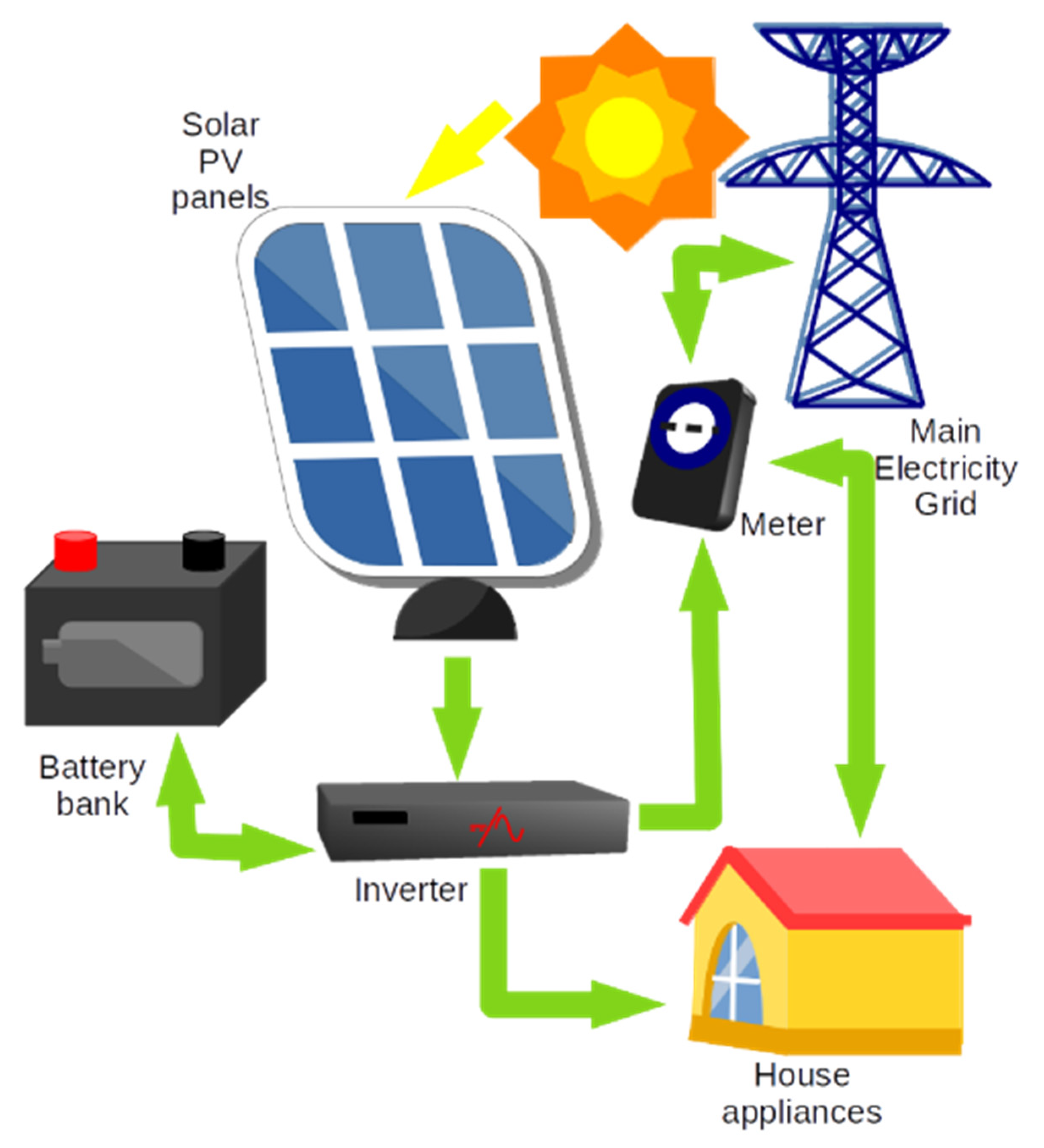
• The proposed model also integrated solar-based renewable-energy resources (RESs). Real data from [25] was used for validation.

2. Cooperative Game Theory

2.1. Overview of Game Theory

Game theory provides a series of analytical tools, which allows us to understand what is observed in decision-making interactions. The foundation of the theory is formed by two basic assumptions: decision-makers are rational, and reason strategically by considering the expectations of other decision-makers’ behaviors. Real-life situations are modeled by game theory through highly abstract representations, thus, allowing their use to study problems in many fields [26].

2.2. Types of Games

There are noncooperative games and cooperative (or coalitional) games. In the former, each action is taken by a single player in response to the other players [27]. In cooperative games, the model consists of the set of joint actions that each group of players (or coalition) can take in response to the other players. Cooperative games are concerned with the interactions among players, the value of each coalition and how the value can be distributed to the participating players.

2.3. Shapley Value

The Shapley Value [28] is a solution concept for coalitional games along with the core, nucleolus and Pareto optimal, among others. Given a coalitional game $\left(\mathcal{N},v\right)$, there is a unique feasible payoff division $x\left(v\right)=\phi \left(\mathcal{N},v\right)$ that divides the full payoff of the grand coalition. The Shapley Value can be defined as [29],

$${\phi }_i\left(\mathcal{N},v\right)=\frac{1}{N!}{\displaystyle \sum }_{R=1}^{N!}\left[v\left(P_i\left(R\right)\cup i\right)-v\left(P_i\left(R\right)\right)\right]$$

(1)

where $R$ is the set of all $N!$ orderings of $\mathcal{N}$, $P_i\left(R\right)$ is the set of players preceding $i$ in the ordering $R$ and ${\phi }_i\left(\mathcal{N},v\right)$ is the expected marginal contribution over all orders of player $i$ to the set of players who are preceding it [26].

The Shapley Value also satisfies the following axioms [30]:

• Symmetry: The symmetry axiom states that interchangeable players $i$ and $j$ should receive the same payments: ${\phi }_i\left(\mathcal{N},v\right)={\phi }_j\left(\mathcal{N},v\right)$. Two agents are interchangeable if they contribute the same amount to every coalition with the other agents.
• Dummy Axiom: The dummy player $i$ contributes to any coalition the same amount that $i$ can achieve alone. Thus, for any $v$, if $i$ is a dummy player, then ${\phi }_i\left(\mathcal{N},v\right)=v\left(i\right)$.
• Additivity: The additivity axiom states that for any two coalitional game problems, defined by $v_1$ and $v_2$, we have for any player $i$ that ${\phi }_i\left(\mathcal{N},v_1+v_2\right)$ = ${\phi }_i\left(\mathcal{N},v_1\right)$ + ${\phi }_i\left(\mathcal{N},v_2\right)$, where the game ${\phi }_i\left(\mathcal{N},v_1+v_2\right)$ is defined by $\left(v_1+v_2\right)\left(S\right)=v_1\left(S\right)+v_2\left(S\right)$ for every coalition $S$.
• Efficiency: The efficiency axioms states that the entire payoff is divided among the players, so $\sum _1^{\mathcal{N}}{\phi }_i=v\left(\mathcal{N}\right)$, where ${\phi }_i$ is the Shapley Value of player $i$.

3. Satisfaction Model

3.1. Satisfaction Concept

The human experience is complex to describe since it depends on the reality of each person. Satisfaction, on the other hand, is a more general concept and describes the user’s perception and how its expectation can be fulfilled [7]. This research proposes a model to quantify satisfaction in the context of a household with different devices. The use of each device provides different levels of satisfaction at different times of the day. Daily moments are captured and summed up to build the energy satisfaction concept. As part of this model, we also consider excessive and poor consumption.

3.2. User Input Satisfaction

The proposed algorithm will be finding the hours of the day for which energy should be allocated to achieve the maximum satisfaction at a minimum energy consumption. For the user satisfaction, it is assumed:

• Satisfaction among devices can be compared at two levels: time-based, satisfaction $\Omega$, and device-based satisfaction Δ, as defined by Ogunjuyigbe [8]. The former implies that if there is a device no. 1, then the satisfaction it is providing at time $t_1$, $\left({\Omega }_1\left(t_1\right)\right)$, can be compared with the satisfaction the same device is providing at different time $t_2$, $({\Omega }_1\left(t_2\right)$). For the latter, if the two devices need to be used at the same time, then there is a satisfaction derived from using device no. 1 $({\Delta }_1\left(t_1\right)$), which can be compared with the satisfaction derived from using device no. 2 $\left({\Delta }_2\left(t_1\right)\right)$ at that hour.
• Time-based satisfaction $\Omega$ has an integer numerical value from zero (0) to six (6), where six (6) means completely satisfied, three (3) means neutral, and small satisfaction values, such zero (0), one (1) and two (2) will denote dissatisfaction.
• Three (3) levels of time-based satisfaction are identified according with these seven (7) scores, see

  Table 1. Levels of Satisfaction.

  Level	Respondent’s Answer
  Satisfied	4, 5, 6
  Neutral	3
  Unsatisfied	0, 1, 2

  .

3.3. Power Satisfaction

The power satisfaction will not only depend on the user input satisfaction set by the household’s head. PS also depends on the energy consumption patterns at each hour of the day. Thus, PS depends on the number of hours of continuous usage (CLoU) and the total length of use in a day (LoU). To find the $PS$ at time $t$, we need to analyze the previous 24 h, i.e., from time $t-24$ until time $t-1$. It is suggested that $PS$ cannot be tested based on how satisfied a person is at t but it will be affected by its perception of the last 24 h.

3.4. Equation of Power Satisfaction

Power satisfaction at a given time/hour can be expressed as the function in Equation (2) below:

$$\begin{array}{l}P{S}_i\left[t\right]=({\alpha }_i\left[t\right]-{\beta }_i\left[t\right]\left|{\widehat{t_u}}_i\left[t\right]-t_{u_i}\right|-\gamma \left[t\right]\left|{\widehat{t_t}}_i\left[t\right]-t_{t_i}\right|)u_i\left[t\right]\end{array}$$

(2)

where,

$${\beta }_i\left[t\right]={\gamma }_i\left[t\right]=\frac{{\alpha }_i\left[t\right]+3}{48-t_{u_i}-t_{t_i}}$$

(3)

where, $\alpha$ is related to the customer’s answer, $\beta$ is related to CLoU and $\gamma$ is the related to LoU. The main idea is to penalize the initial satisfaction, $\alpha$ according to an excess or poor consumption. Variables $\beta$ and $\gamma$ depends on $\alpha$ and convert $\widehat{t_u}$ and $\widehat{t_t}$, respectively, into a value that can be deducted from α and,

$${\alpha }_i\left[t\right]=\frac{{\Omega }_i\left[t\right]}{t_{t_i}},$$

(4)

where ${\Omega }_i$ is the time-based input satisfaction for device $i$ and it is divided by the responsible LoU, $t_{t_i}$, hence $\alpha$ will reach its maximum if it used the expected time $t_{t_i}$ hours during a 24-h period. To find PS, 24 h of experiment is needed. For each device $i$, the array ${\mathit{u}}_{\mathit{i}}=\left\{u_n:n=1,2,\dots 24\right\}$ where $u_n$ is 0 or 1. It is the input vector for each device with the operational status of the devices, it will be one (1) when ‘ON’ and (0) if it is ‘OFF’. For further details, see previous work reference [19].

3.5. Energy Satisfaction

Each user has a subset $\left\{i:i=1,2,\dots ,N\right\}$ of $N$ participant devices. Following the well-known concept of electric energy, to find the energy satisfaction, $ES$, in time $t$, the previous 24 values of $PS$ are required, i.e., $\left\{P{S}_i\left[t-24\right],\dots ,P{S}_i\left[t-1\right]\right\}$. To compute the first $PS$, $P{S}_i\left[t-24\right]$, the past 24 h before this time are also required. Hence, to compute ES, 48 h of experiment are required. $ES$ is defined as in Equation (5).

$$ES\left[t\right]=\frac{1}{N}{\displaystyle \sum }_{i\in N}{\displaystyle \sum }_{n=k}P{S}_{i,n},$$

(5)

where $N$ is the number of participant devices, $k$ is the initial time of the experiment, $t=k+23$ and ${\Delta }_{i,t}$ is the device-based satisfaction.

Equation (5) is modified to include the concept of device-based satisfaction $\Delta$. ES becomes a weighted summation and reflects the specific needs at that current time $t$. Subsequently, the average is computed to obtain the $ES$ value at time $t$,

$$E{S}^{\prime }\left[t\right]=\frac{1}{N}\left({\displaystyle \sum }_{i\in N}{\Delta }_{i,t}P{S}_{i,t}+\left({\displaystyle \sum }_{n=k}^{t-1}P{S}_{i,n}\right)\right),$$

(6)

4. Problem Formulation

4.1. Electric Energy Function

The energy consumption in an hour from time $t$ until time $t+1$ is defined as in Equation (7),

$$L\left[t\right]={\displaystyle \sum }_{i\in N}{e}_{i,t}{u}_i\left[t\right],$$

(7)

where $e_{i,t}$ represents an usual energy consumption of device $i$ in one hour and ${\mathit{u}}_{\mathit{i}}$ is the input vector for each device $i$ with its operational status. It will be one (1) when ‘ON’ and zero (0) if it is ‘OFF’.

4.2. Optimization Problem

The problem of jointly maximizing the satisfaction while minimizing the power consumption $f_2\left(u\right)$ can be formulated as a multi-objective (MOO) problem:

$$min\left[f_1\left(u,t\right),-f_2\left(u,t\right)\right],$$

(8)

$$s.t.L\left[t\right]\le E_{con},$$

(9)

where,

$$f_1\left(t,u\right)=L\left[t\right],$$

(10)

$$f_2\left(t,u\right)=E{S}^{\prime }\left[t\right],$$

(11)

$$t\in \left\{k,k+1,\dots ,k+23\right\}$$

(12)

4.3. Constraint

The algorithm is subjected to the constraint that the total energy consumption of the user is less or equal to a pre-defined energy budget, $E_{con}$,

$$s.t.L\left[t\right]\le E_{con},$$

(13)

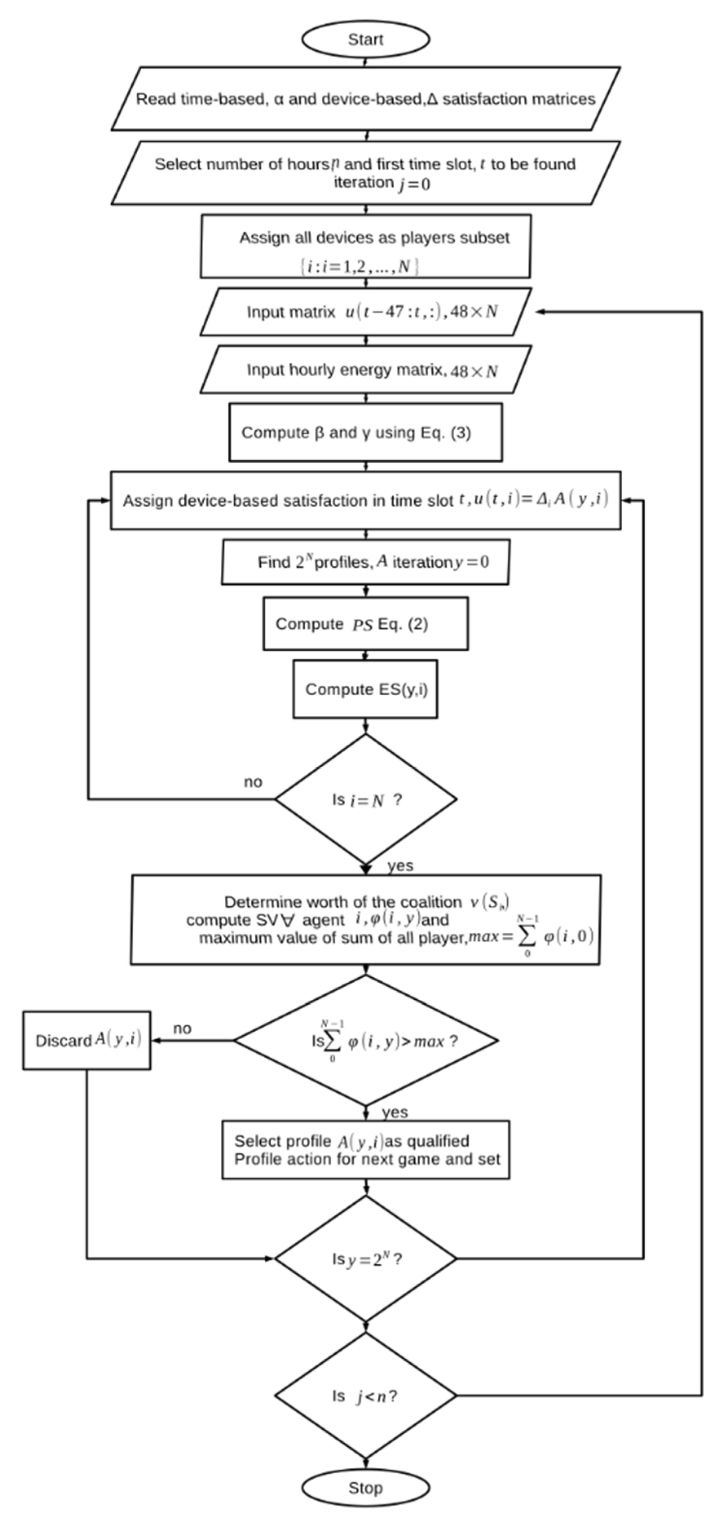
4.4. Cooperative Game Model Implementation

A mathematical model based on cooperative game theory is developed to capture the complex interactions among the different devices. The Shapley Value algorithm based on the cooperative game implementation is applied to all participating devices to obtain the ${\mathit{u}}_{\mathit{i}}$ vector. Such that energy can be allocated to simultaneously maximize the $E{S}^{\prime }$ and minimize the energy consumption $L$ for a corresponding energy reference. The flow chart for the proposed algorithm is shown in Figure 1. Time-based and device-based satisfaction tables and power consumption for each device are established. The proposed approach is to design a consumption scheduling for a selected number of hours $n$. Additionally, we should decide time $t$ to start the experiment and the number N of participating devices. Considering the experiment should collect energy data for the 48 h before this time t, then the status matrix is of size $48\times N$. The number of possible action profiles $A$, is found ($2^N$). Since each possible action profile contains the possible devices´ status, each of these possible profiles are multiplied for the correspondent Device-based satisfaction $\Delta$ according to the time of the day and the device. $PS$ and $ES$ are computed using Equations (2) and (6) at each time slot, respectively. Next, the worth of the coalition $v\left(S_k\right)$ can be found for each time slot for each profile. Lastly, the group of actions with maximum SV can be selected.

To implement this algorithm the following considerations are followed:

• Players:

Devices-agents $i=1,2,\dots ,N$ are considered the players.

• Actions:

Devices can be ON or OFF, so the actions would be turning ON or OFF the participant devices (players.) The ${\mathit{u}}_{\mathit{i}}$ array will be zeros or one depending on the device status.

• Payoffs:

Consumption and ES are combined and modeled as optimization function using the characteristic function.

• Value of coalition:

Agents form coalitions and every coalition and corresponding actions have different value. For $K\subseteq N$, $S_K$ is the group of $K$ devices that agreed to make a coalition to maximize the total expected payoff $v\left(S_K\right)$ that they can achieve together. The value of a coalition for this cooperative game is,

$$v{\left(S_K\right)}_t=\{\begin{array}{c}0,|L\left[t\right]>E_{ref}\cap E{S}^{\prime }\left[t\right]<4\\ \left[1-f\left|\frac{L\left[t\right]-P_{PV}\left[t\right]}{max\left(L\left[t\right],P_{PV}\left[t\right]\right)}\right|\right]\left[\frac{ES\left[t\right]}{6}\right],P_{PV}\left[t\right]<L\left[t\right]<E_{ref}\\ \left[1-\left|\frac{L\left[t\right]-P_{PV}\left[t\right]}{max\left(L\left[t\right],P_{PV}\left[t\right]\right)}\right|\right]\left[\frac{ES\left[t\right]}{6}\right]otherwise\end{array},$$

(14)

where $f$ is a factor to penalize level of consumption among the energy reference and solar energy less than cases when less then solar energy and $P_{PV}\left[t\right]$ is the minimum among the set of power output of generation($P_{pv}\left[t\right]$) and the power inverter ($P_{inv}\left[t\right]),$ i.e., $P_{PV}\left[t\right]=min\left(P_{pv}\left[t\right],P_{inv}\left[t\right]\right)$, for the cases with just utility and $P_{PV}\left[t\right]=min\left(P_{pv}\left[t\right]+P_{bat},P_{inv}\left[t\right]\right)$ for the cases with batteries and utility, where $P_{bat}$ is the set of power output from batteries.

There are three levels of consumption: $L\le P_{PV},P_{PV}<L\le E_{ref}$ and $L>E_{ref}$. Where $E_{ref}$ would be a consumption that is acceptable, there will be penalty if it is less than $P_{PV}$ or greater than $E_{ref}$.

5. Experimental Results and Discussion

5.1. Case Study: House with Photovolatic System (PV) and Utility or House with PV, Batteries and Utility

The proposed model is being validated by representing a single rural residential house that may contain a small photovoltaic (PV) system that is composed of one or more solar panels combined, a DC/AC inverter, and it is grid-connected. Figure 2 describes a generalized version of the system. Energy data to simulate the case study is obtained in two ways:

• Reference Energy Disaggregation Data Set (REDD) [31] for power ratings and status vector (u_i) for refrigerator, microwave, lighting, stove, and water heater.
• Power ratings for TV, AC, Radio and phone, are obtained from Ogunjuyigbe [8]. Status vectors for these four devices are randomly generated.

5.2. Data Characterization for the Algorithm Calibration

5.2.1. Household’s Load

For the load data, a single house’s devices (four of them) are analyzed, the REDD data [31] is used to represent a part of house’s loads. Data that is shown in

Table 2. Load Description.

Device	Rating (W)	tu	tt
Lightings	240	4	8
Refrigerator	170	24	24
Stove	2	3	9
Microwave (Oven)	1200	1	4

contains average power reading for the individual circuits of the house. The REDD data was sampled every three seconds. Hence, there are 20 data points per minute. The ${\mathit{u}}_{\mathit{i}}$ array is an hourly vector. For this vector, it needs to be decided how much time within an hour a certain device must be ON to assign a one (1) in that time slot.

5.2.2. House Head’s Satisfaction

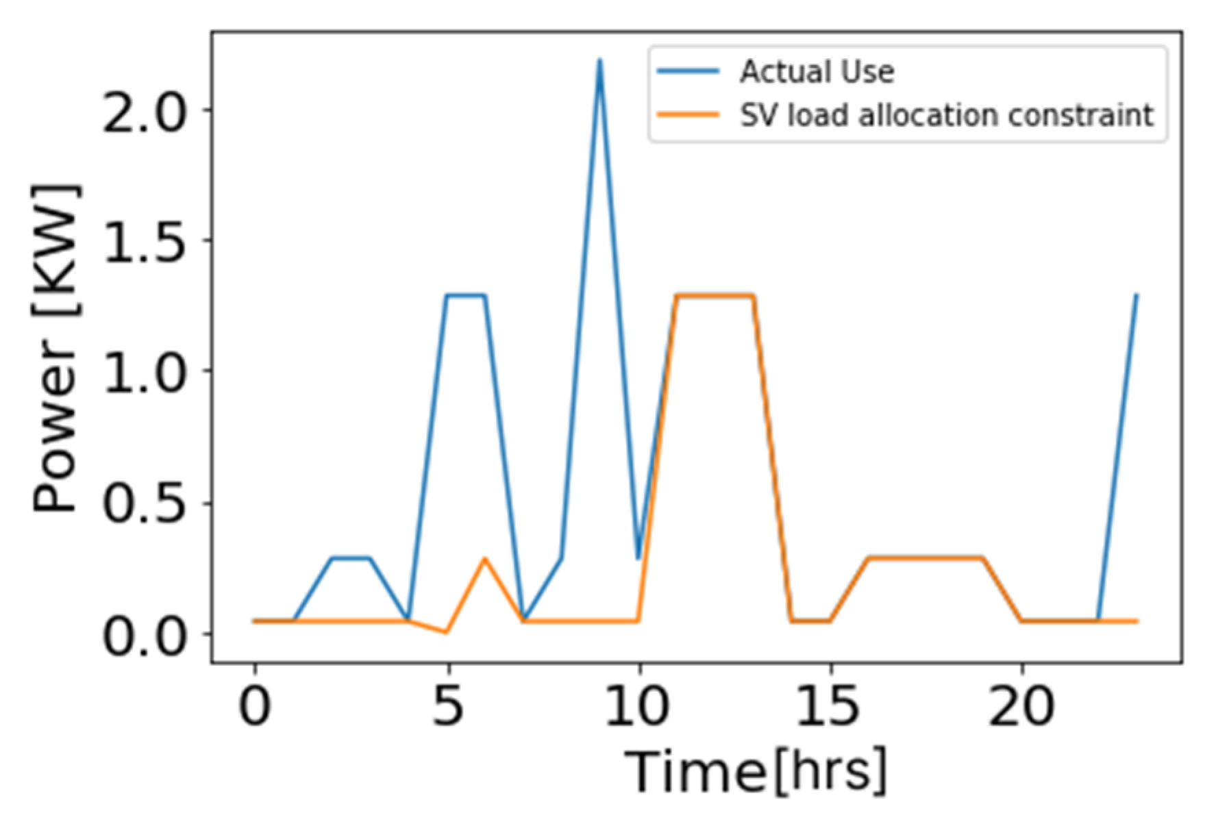
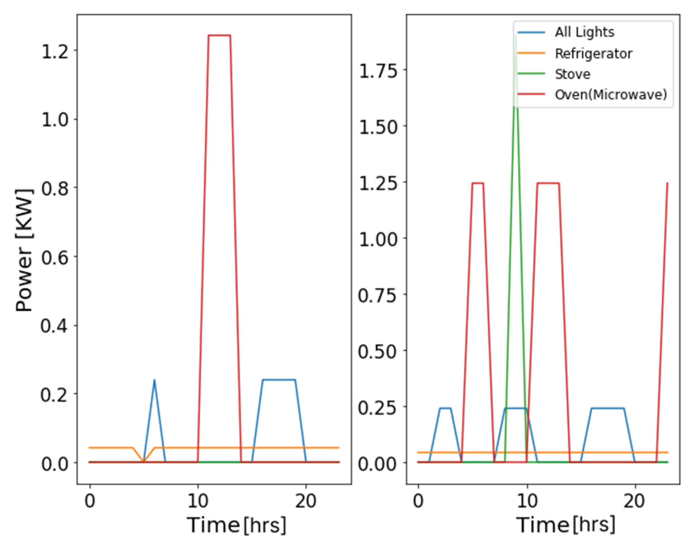
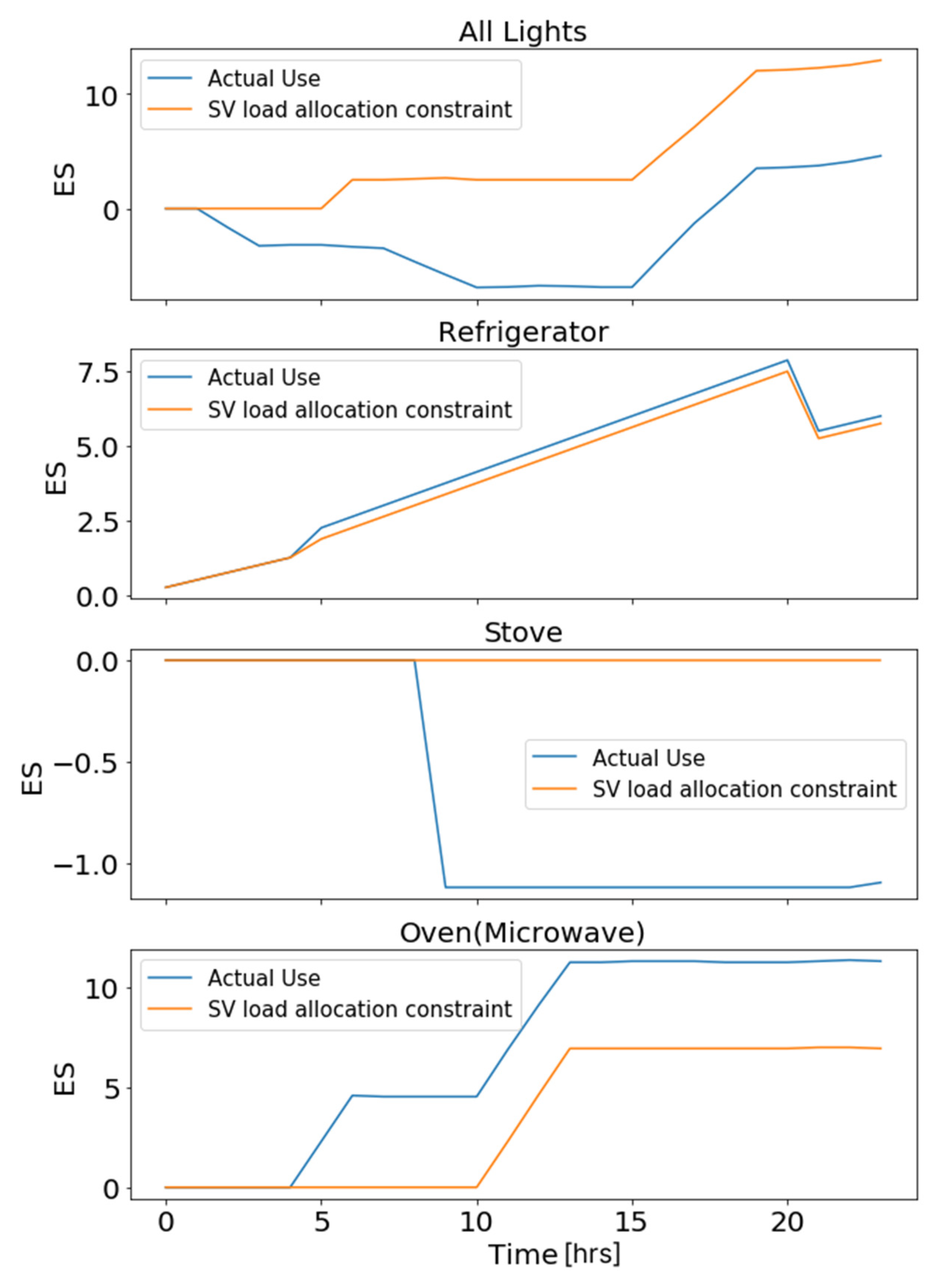
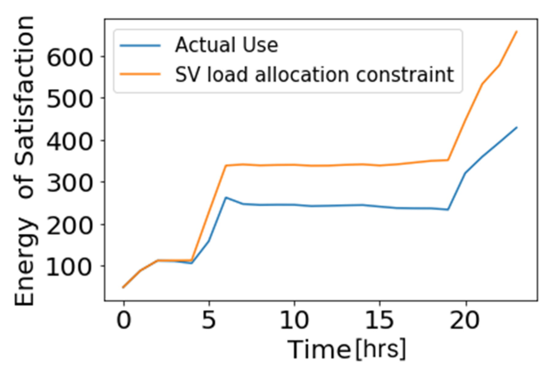
Satisfaction matrices were generated according to author’s personal experience and they are described in

Table 3. Time-based satisfaction.

S/N	Equipment	Hours
		1	2	3	4	5	6	7	8	9	10	11	12	13	14	15	16	17	18	19	20	21	22	23	24
1	Lightings	−3	−3	−3	−3	−3	6	6	6	−2	−2	−2	−2	−2	−2	−2	−2	6	6	6	6	6	−3	−3	−3
2	Refrigerator	4	4	4	4	4	6	6	6	6	6	6	6	6	6	6	6	6	6	6	6	6	4	4	4
3	Stove	−2	−2	−2	−2	−2	6	6	6	−2	−2	−2	5	6	6	5	−2	−2	−2	−2	6	6	−2	−2	−2
4	Microwave	4	4	0	0	0	6	6	6	6	0	0	6	6	6	0	0	0	0	6	6	6	0	0	0

and

Table 4. Device-based satisfaction.

S/N	Equipment	Hours
		1	2	3	4	5	6	7	8	9	10	11	12	13	14	15	16	17	18	19	20	21	22	23	24
1	Lightings	4	4	4	4	4	4	4	4	4	4	4	4	4	4	4	4	4	4	4	4	4	4	4	4
2	Refrigerator	1	1	1	1	1	1	1	1	1	1	1	1	1	1	1	1	1	1	1	1	1	1	1	1
3	Stove	−2	−2	−2	−2	−2	−2	−2	−2	−2	−2	−2	−2	−2	−2	−2	−2	−2	−2	−2	−2	−2	−2	−2	−2
4	Microwave	4	4	4	4	4	4	4	4	4	4	4	4	4	4	4	4	4	4	4	4	4	4	4	4

. This first stage of results is simply used as a sanity check. In the Section 5.3, actual load description (see

Table 5. Load description.

Device	Rating (W)	tu	tt
Lightings	135	4	8
Microwave (Oven)	1200	1	4
TV	200	2	4
AC	800	6	8
Radio	50	5	12
Water Heater	2000	1	2
Laptop	100	8	12
Phone	10	1	3

) is used for each device based on REDD database and Ogunjuyigbe et al.’s [8] work. Besides, actual values of satisfaction were used to generate

Table 6. Time-based satisfaction.

S/N	Equipment	Hours
		1	2	3	4	5	6	7	8	9	10	11	12	13	14	15	16	17	18	19	20	21	22	23	24
1	TV	0.0	0.0	0.0	0.0	0.0	0.0	−2.4	−2.4	0.0	0.0	0.0	0.0	0.0	0.0	−2.4	−2.4	−2.4	−1.8	4.4	6.0	6.0	5.2	4.4	−0.6
2	Lighting	0.0	0.0	0.0	0.0	0.0	4.8	4.0	−0.6	−2.4	0.0	0.0	0.0	0.0	0.0	0.0	0.0	−1.2	4.0	4.4	6.0	6.0	5.2	4.4	−1.2
3	AC	0.0	0.0	0.0	0.0	−2.4	−0.6	−1.8	−2.4	0.0	0.0	0.0	0.0	0.0	0.0	0.0	0.0	−2.4	−1.2	−1.2	4.4	6.0	6.0	−1.8	−2.4
4	Radio	0.0	0.0	0.0	0.0	−2.4	−1.8	6.0	−1.8	−1.8	−2.4	0.0	0.0	0.0	0.0	0.0	0.0	0.0	0.0	−2.4	−1.8	−1.8	0.0	0.0	0.0
5	Water Heater	0.0	0.0	0.0	−2.4	−1.2	6.0	4.0	−1.8	−2.4	0.0	0.0	0.0	0.0	0.0	0.0	0.0	0.0	0.0	0.0	0.0	0.0	0.0	0.0	0.0
6	Lighting	0.0	0.0	0.0	0.0	−1.2	6.0	−1.2	−1.8	−2.4	0.0	0.0	0.0	0.0	0.0	0.0	0.0	0.0	−1.8	−2.4	−1.8	6.0	4.0	−1.2	−1.8
7	Microwave Oven	0.0	0.0	0.0	0.0	−2.4	6.0	6.0	−2.4	0.0	0.0	0.0	0.0	0.0	0.0	0.0	0.0	−2.4	−2.4	4.8	6.0	−1.2	−2.4	0.0	0.0
8	Lighting	0.0	0.0	0.0	0.0	−1.2	6.0	4.0	−1.2	−2.4	0.0	0.0	0.0	0.0	0.0	0.0	0.0	0.0	−2.4	4.8	6.0	−0.6	−1.8	−2.4	0.0
9	Lighting	6.0	6.0	5.6	5.2	4.8	4.4	−1.2	−2.4	0.0	0.0	0.0	0.0	0.0	0.0	0.0	0.0	0.0	−2.4	−1.8	4.0	4.8	5.2	5.6	6.0
10	Lighting	0.0	0.0	0.0	0.0	−1.8	6.0	4.8	−1.2	−2.4	0.0	0.0	0.0	0.0	0.0	0.0	0.0	0.0	−2.4	−1.8	−0.6	4.0	4.8	6.0	−0.6
11	Laptop	0.0	0.0	0.0	0.0	−2.4	4.0	−1.2	−2.4	−2.4	0.0	0.0	0.0	0.0	0.0	0.0	0.0	0.0	0.0	−2.4	−2.4	−1.2	4.0	6.0	5.2
12	Phone	6.0	4.8	4.4	−0.6	−1.2	−1.2	−1.8	−2.4	0.0	0.0	0.0	0.0	0.0	0.0	0.0	0.0	0.0	0.0	−2.4	−2.4	−2.4	−1.2	4.0	6.0

and

Table 7. Device-based satisfaction.

S/N	Equipment	Hours
		1	2	3	4	5	6	7	8	9	10	11	12	13	14	15	16	17	18	19	20	21	22	23	24
1	TV	0.0	0.0	0.0	0.0	0.0	0.0	−2.4	−2.4	0.0	0.0	0.0	0.0	0.0	0.0	−2.4	−2.4	−2.4	−1.8	4.4	6.0	6.0	5.2	4.4	−0.6
2	Lighting	0.0	0.0	0.0	0.0	0.0	4.8	4.0	−0.6	−2.4	0.0	0.0	0.0	0.0	0.0	0.0	0.0	−1.2	4.0	4.4	6.0	6.0	5.2	4.4	−1.2
3	AC	0.0	0.0	0.0	0.0	−2.4	−0.6	−1.8	−2.4	0.0	0.0	0.0	0.0	0.0	0.0	0.0	0.0	−2.4	−1.2	−1.2	4.4	6.0	6.0	−1.8	−2.4
4	Radio	0.0	0.0	0.0	0.0	−2.4	−1.8	6.0	−1.8	−1.8	−2.4	0.0	0.0	0.0	0.0	0.0	0.0	0.0	0.0	−2.4	−1.8	−1.8	0.0	0.0	0.0
5	Water Heater	0.0	0.0	0.0	−2.4	−1.2	6.0	4.0	−1.8	−2.4	0.0	0.0	0.0	0.0	0.0	0.0	0.0	0.0	0.0	0.0	0.0	0.0	0.0	0.0	0.0
6	Lighting	0.0	0.0	0.0	0.0	−1.2	6.0	−1.2	−1.8	−2.4	0.0	0.0	0.0	0.0	0.0	0.0	0.0	0.0	−1.8	−2.4	−1.8	6.0	4.0	−1.2	−1.8
7	Microwave Oven	0.0	0.0	0.0	0.0	−2.4	6.0	6.0	−2.4	0.0	0.0	0.0	0.0	0.0	0.0	0.0	0.0	−2.4	−2.4	4.8	6.0	−1.2	−2.4	0.0	0.0
8	Lighting	0.0	0.0	0.0	0.0	−1.2	6.0	4.0	−1.2	−2.4	0.0	0.0	0.0	0.0	0.0	0.0	0.0	0.0	−2.4	4.8	6.0	−0.6	−1.8	−2.4	0.0
9	Lighting	6.0	6.0	5.6	5.2	4.8	4.4	−1.2	−2.4	0.0	0.0	0.0	0.0	0.0	0.0	0.0	0.0	0.0	−2.4	−1.8	4.0	4.8	5.2	5.6	6.0
10	Lighting	0.0	0.0	0.0	0.0	−1.8	6.0	4.8	−1.2	−2.4	0.0	0.0	0.0	0.0	0.0	0.0	0.0	0.0	−2.4	−1.8	−0.6	4.0	4.8	6.0	−0.6
11	Laptop	0.0	0.0	0.0	0.0	−2.4	4.0	−1.2	−2.4	−2.4	0.0	0.0	0.0	0.0	0.0	0.0	0.0	0.0	0.0	−2.4	−2.4	−1.2	4.0	6.0	5.2
12	Phone	6.0	4.8	4.4	−0.6	−1.2	−1.2	−1.8	−2.4	0.0	0.0	0.0	0.0	0.0	0.0	0.0	0.0	0.0	0.0	−2.4	−2.4	−2.4	−1.2	4.0	6.0

. The authors´ personal experience reflects and summarizes how devices were prioritized by most of the population in extreme conditions such as those experienced after hurricane Maria in 2017 in Puerto Rico. However, future work will include field data to build the time-based satisfaction and device-based satisfaction tables.

5.2.3. Results

Figure 3 depicts the amount of energy used by each of the four devices under the proposed SV allocation algorithm and the actual energy usage according to the REDD database [31]. The proposed optimization problem has been constrained. Thus, showing how with the same amount or less energy than in the actual REDD scenario. ES (see Figure 4) is higher at each time slot.

Figure 5 depicts how power is used in both scenarios. Figure 6 shows the resulting ES from that energy usage. Lighting is suggested to be on early in the morning and in the afternoon when the satisfaction derived from them is the highest. Therefore, the refrigerator needs to be off for one hour because it is a priority (see Table 4 to have lighting on since its contribution to the total ES is higher. However, analyzing ES brought by refrigerator in Figure 6 is slightly lower for the proposed algorithm since it was turned off. According to the REDD database [31], the stove is in on status during one hour but it is on at a time that is not bringing any satisfaction, hence the proposed algorithm recommends to not turn it on under the energy restrictions. For the microwave, in the REDD database [31], it is on at different times of the day however it is not on when the satisfaction is the highest. For example, in the morning it is preferable to have lighting on instead of the microwave, since the energy usage of lighting is less than the energy usage of the microwave.

For the calibration part, we made sure the algorithm was suggesting those profiles where the Energy Satisfaction was highest at a minimum energy usage. In the following section, we will be testing the algorithm for a different set of devices.

5.3. Data Characterization for the Algorithm Testing.

Eight devices were selected according to the ones used in Ogunjuyigbe et al. [8] for testing purposes. For the algorithm simplicity, all lights were considered as a single appliance. Ogunjuyigbe et al. [8] used some loads for which there are not data available in the REDD database [31], such as TV, AC, Radio, and phone. Hence, for these ones, Unit Wattage data from [8] was used. Additionally, ${\mathit{u}}_{\mathit{i}}$ was randomly generated for those devices, such that a comparison can be made with the proposed algorithm’s ${\mathit{u}}_{\mathit{i}}$ output. Table 5 describes the electrical appliances used by a user, their rating, their optimum CLoU, $t_u$ and their optimum LoU, $t_t$ for a responsible consumption.

5.3.1. House Head’s Satisfaction

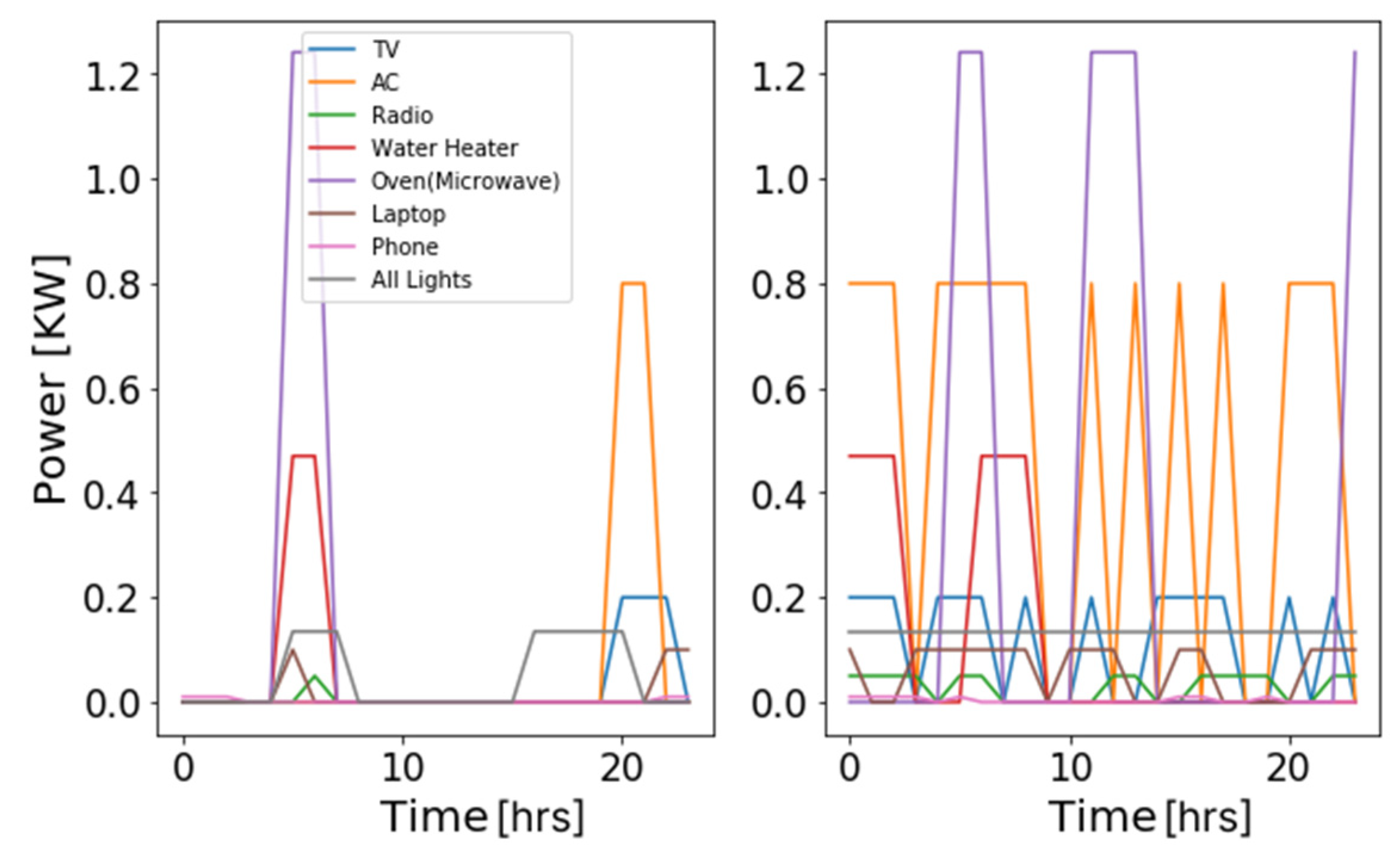
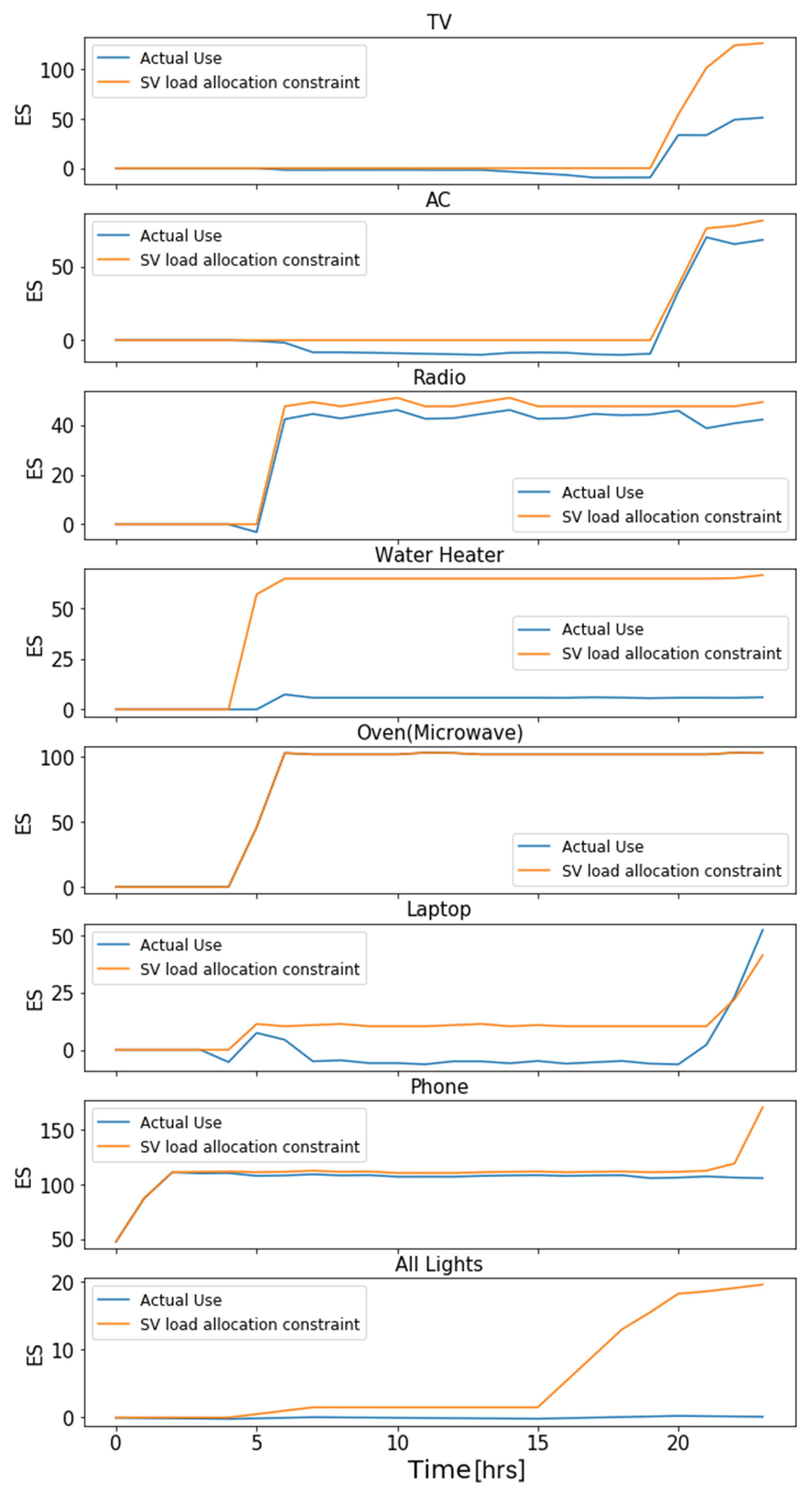
The algorithm also needs practical input data for satisfaction to create the model. Data from Ogunjuyigbe et al. [8] $({\sigma }^t$ and ${\sigma }^d$) are being used for this purpose. Data from time-based satisfaction was mapped into satisfaction levels described in Table 1 in the following fashion,

$${\Omega }_t=\{\begin{array}{c}0,if{\sigma }^t=0.5\\ 6-\frac{2\left(1-{\sigma }^t\left[t\right]\right)}{0.5},if{\sigma }^t\ge 0.5\\ 6{\sigma }^t\left[t\right]-3,if{\sigma }^t<0.5\end{array},$$

(15)

Dissatisfaction and ‘indifference’ values (0, 1, 2 and 3) are mapped into negative values and zero (−3, −2, −1 and 0, respectively). The proposed model introduced negative values when low satisfaction, thus making it preferable to have them ‘OFF’, representing by itself, before the optimization problem, a more accurate satisfaction model, which allows making decisions not only for energy and economic savings but also responsibly fulfilling the customer’s satisfaction. Table 6 shows complete resulting time-based satisfaction table and Table 7 shows device-based satisfaction after mapping d-domain satisfaction found in Ogunjuyigbe et al. [8] (${\sigma }^d$) by using Equation (16).

$$\Delta \left[t\right]=10{\sigma }^d\left[t\right],$$

(16)

5.3.2. Results

One of the main results to report is that the implementation of the SV optimization provided a consumption pattern that represents an energy consumption less or equal than the initial actual use and a higher energy satisfaction for almost all hours in all devices. Figure 7 provides the graphical comparison of the power consumption at each hour for the actual based case and the case with the SV optimization. Figure 8 presents the energy satisfaction at each hour showing how the SV optimization outperforms the base case, particularly increasing its advantage in the early morning hours and the late evening hours.

Figure 9 depicts a comparison of the hourly power consumption of all devices between the proposed SV allocation algorithm and the actual power consumption. In Figure 9 (left side), the algorithm attempts to meet desired time-based and device-based satisfaction tables (See Table 6 and Table 7) while consuming equal or less hourly power than the one shown in 9 (right side). The energy reduction was of approximately 75%, from 32.6 KWh to 7.35 KWh. Equally important is the energy satisfaction increase of 40% with the SV algorithm, from 5500 to 7825. A consumption plan is scheduled for the user by managing devices based on the SV game theory approach. Next, a reliability signal or economic signal will be sent to a Human-Machine Interface (HMI). A reliability signal will ensure that the electric system keeps operating when a house is not connected to the grid, while an economic signal ensures the same purpose when connected to the grid. This way, the customer is aware of the situation and can make a final decision based on the available information.

Figure 10 includes the ES for each device and it seems that the better SV performance is due mainly to the microwave use in the morning and the TV at night. Since operational status vectors, $\mathit{u}$ for TV, AC, Radio, and phone, were randomly generated, Figure 9 shows an atypical consumption pattern. Figure 10 shows a comparison between the hourly ES obtained through the SV allocation algorithm and the ES obtained in the actual case representation, for each of the devices. When attempting to meet the energy constraints imposed by the actual case scenario, with the proposed SV algorithm, the ES obtained at each hour is equal or higher for almost each of the hours for every device. This is one of the most important results of this study. Only in the case of the laptop, the ES is higher at the last hour of the day in the actual case scenario.

Similarly, Ogunjuyigbe et al. [8] presented their results in 24 h plots for three different daily budget constraints to provide a maximum satisfaction at those predefined budgets. On the other hand, the present research used energy constraints rather than budget, and thus including a key component of the research when penalizing excessive and low consumption, because of its detrimental impact in the quality of life. He compared a ‘desired satisfaction’ with an ‘achieved satisfaction’. The ‘achieved satisfaction’ was the output of their load-satisfaction algorithm, which is analogous to the present ‘SV load allocation’ algorithm. We did not choose to compare the output results with the ‘desired satisfaction’ (as Seen in Table 6 and Table 7). Instead, we compare it with an ‘actual’ scenario represented by using the REDD database. Ogunjuyigbe et al. [8] implemented a genetic algorithm (GA) approach. While the GA approach may have a good convergence speed and good efficiency, the present approach does not have to deal with convergence times and offers a more intuitive optimization framework.

6. Conclusions

A novel model to include customer’s satisfaction in an optimization problem was introduced. A quantifiable user satisfaction was developed. The satisfaction concept through the novel concepts of power satisfaction (PS) and energy satisfaction (ES) included the detrimental impact that excess consumption could have in the quality of life. The algorithm provided the hours of the day for which the energy should be allocated to achieve maximum satisfaction at an energy constraint imposed by the energy consumption in actual case scenarios. Actual case scenarios were represented by using the REDD database. The Shapley Value (SV) concept from the game theory framework was implemented to obtain a recommendation on how energy should be allocated. The results showed how the algorithm maximized user´s ES at a minimum energy consumption. The proposed approach reduced energy consumption 75%, while increasing ES 40%.

SV-based optimization successfully achieved to maximize satisfaction at a minimum energy consumption although it also has high computational complexity. Further work can be done to decrease computational complexity and thus the required reduction processing times. This could be achieved by using more powerful computers or through the derivation recursive and/or parallel implementation of the proposed algorithm. The proposed methodology is validated by simulating a rural single house with limited resources connected to the grid. It should be pointed out that the satisfaction model can be readily applied in a real case scenario of rural communities.

References

1. Access to Energy|Sustainable Energy for All. Available online: https://www.seforall.org/goal-7-targets/access (accessed on 24 February 2021).
2. Wu, Q.; Ren, H.; Gao, W.; Ren, J. Benefit allocation for distributed energy network participants applying game theory based solutions. Energy 2017, 119, 384–391. [Google Scholar] [CrossRef]
3. Tang, R.; Wang, S.; Wang, H. Optimal power demand management for cluster-level commercial buildings using the game theoretic method. Energy Procedia 2019, 159, 186–191. [Google Scholar] [CrossRef]
4. Lokeshgupta, B.; Sivasubramani, S. Cooperative game theory approach for multi-objective home energy management with renewable energy integration. IET Smart Grid 2019, 2, 34–41. [Google Scholar] [CrossRef]
5. Yang, P.; Tang, G.; Nehorai, A. A game-theoretic approach for optimal time-of-use electricity pricing. IEEE Trans. Power Syst. 2012, 28, 884–892. [Google Scholar] [CrossRef]
6. Marzband, M.; Ardeshiri, R.R.; Moafi, M.; Uppal, H. Distributed generation for economic benefit maximization through coalition formation–based game theory concept. Int. Trans. Electr. Energy Syst. 2017, 27, e2313. [Google Scholar] [CrossRef]
7. Shahzad, S.; Brennan, J.; Theodossopoulos, D.; Hughes, B.; Calautit, J.K. Energy and comfort in contemporary open plan and traditional personal offices. Appl. Energy 2017, 185, 1542–1555. [Google Scholar] [CrossRef]
8. Ogunjuyigbe, A.S.O.; Ayodele, T.R.; Akinola, O.A. User satisfaction-induced demand side load management in residential buildings with user budget constraint. Appl. Energy 2017, 187, 352–366. [Google Scholar] [CrossRef]
9. Yoon, S.G.; Choi, Y.J.; Park, J.K.; Bahk, S. Stackelberg-Game-Based Demand Response for At-Home Electric Vehicle Charging. IEEE Trans. Veh. Technol. 2016, 65, 4172–4184. [Google Scholar] [CrossRef]
10. Yu, M.; Hong, S.H. A Real-Time Demand-Response Algorithm for Smart Grids: A Stackelberg Game Approach. IEEE Trans. Smart Grid 2016, 7, 879–888. [Google Scholar] [CrossRef]
11. Azimian, B.; Fijani, R.F.; Ghotbi, E.; Wang, X. Stackelberg game approach on modeling of supply demand behavior considering BEV uncertainty. In Proceedings of the 2018 IEEE International Conference on Probabilistic Methods Applied to Power Systems (PMAPS), Boise, ID, USA, 24–28 June 2018. [Google Scholar] [CrossRef]
12. Jia, L.; Tong, L. Dynamic Pricing and Distributed Energy Management for Demand Response. IEEE Trans. Smart Grid 2016, 7, 1128–1136. [Google Scholar] [CrossRef]
13. Ma, L.; Liu, N.; Wang, L.; Zhang, J.; Lei, J.; Zeng, Z.; Wang, C.; Cheng, M. Multi-party energy management for smart building cluster with PV systems using automatic demand response. Energy Build. 2016, 121, 11–21. [Google Scholar] [CrossRef]
14. Agyeman, K.; Han, S.; Han, S. Real-Time Recognition Non-Intrusive Electrical Appliance Monitoring Algorithm for a Residential Building Energy Management System. Energies 2015, 8, 9029–9048. [Google Scholar] [CrossRef]
15. Pal, S.; Thakur, S.; Kumar, R.; Panigrahi, B.K. A strategical game theoretic based demand response model for residential consumers in a fair environment. Int. J. Electr. Power Energy Syst. 2018, 97, 201–210. [Google Scholar] [CrossRef]
16. Wang, Z.; Paranjape, R. Optimal Residential Demand Response for Multiple Heterogeneous Homes with Real-Time Price Prediction in a Multiagent Framework. IEEE Trans. Smart Grid 2017, 8, 1173–1184. [Google Scholar] [CrossRef]
17. Buchanan, K.; Banks, N.; Preston, I.; Russo, R. Corrigendum to The British public’s perception of the UK smart metering initiative: Threats and opportunities. Energy Policy 2016, 91, 87–97. [Google Scholar] [CrossRef] [Green Version]
18. Aked, J.; Cordon, C.; Marks, N. Five Ways to Wellbeing: A report Oresented to The Foresight Project on Communicating the Evidence Base for Improving People’s Well-Being|Repository for Arts and Health Resources. Available online: https://www.artshealthresources.org.uk/docs/five-ways-to-wellbeing-a-report-presented-to-the-foresight-project-on-communicating-the-evidence-base-for-improving-peoples-well-being/ (accessed on 5 February 2021).
19. Ortiz, S.; Ndoye, M.; Castro-Sitiriche, M. Toward an Energy Threshold Hypothesis Model for Social Benefit and Household Energy Usage. In Proceedings of the International Conference on Appropriate Technology 2020, Pretoria, South Africa, 23–27 November 2020; pp. 346–355. [Google Scholar]
20. Sarker, E.; Halder, P.; Seyedmahmoudian, M.; Jamei, E.; Horan, B.; Mekhilef, S.; Stojcevski, A. Progress on the demand side management in smart grid and optimization approaches. Int. J. Energy Res. 2021, 45, 36–64. [Google Scholar] [CrossRef]
21. Tzanetos, A.; Dounias, G. Nature inspired optimization algorithms or simply variations of metaheuristics? Artif. Intell. Rev. 2020. [Google Scholar] [CrossRef]
22. Robert, C. Editorial: Responsible well-being—A personal agenda for development. World Dev. 1997, 25, 1743–1754. Available online: https://ideas.repec.org/a/eee/wdevel/v25y1997i11p1743-1754.html (accessed on 5 February 2021).
23. Castro-Sitiriche, M.J.; Ndoye, M. On the Links between Sustainable Wellbeing and Electric Energy Consumption. Afr. J. Sci. Technol. Innov. Dev. 2013, 5, 327–335. [Google Scholar] [CrossRef]
24. Max-Neef, M. Economic growth and quality of life: A threshold hypothesis. Ecol. Econ. 1995, 15, 115–118. [Google Scholar] [CrossRef]
25. NREL. Solar Resource Data. Jurutungo Community, Puerto Rico. Available online: https://pvwatts.nrel.gov/pvwatts.php (accessed on 11 November 2020).
26. Osborne, M.J.; Rubinstein, A. A Course in Game Theory; The MIT Press: Cambridge, MA, USA, 2011. [Google Scholar]
27. O’Brien, G.; El Gamal, A.; Rajagopal, R. Shapley Value Estimation for Compensation of Participants in Demand Response Programs. IEEE Trans. Smart Grid 2015, 6, 2837–2844. [Google Scholar] [CrossRef]
28. Jackson, M.O.; Leyton-Brown, K.; Yoav, S. Game Theory Online. Available online: http://game-theory-class.org/game-theory-I.html (accessed on 24 February 2021).
29. Arif, M.A.; Ndoye, M.; Murphy, G.V.; Aganah, K. A cooperative game theory algorithm for distributed reactive power reserve optimization and voltage profile improvement. In Proceedings of the 2017 North American Power Symposium (NAPS), Morgantown, WV, USA, 17–19 September 2017. [Google Scholar] [CrossRef]
30. Leyton-Brown, K.; Shoham, Y. Essentials of Game Theory: A Concise Multidisciplinary Introduction. Synth. Lect. Artif. Intell. Mach. Learn. 2008, 2, 1–88. [Google Scholar] [CrossRef] [Green Version]
31. Kolter, J.Z.; Batra, S.; Ng, A.Y. Energy disaggregation via discriminative sparse coding. In Proceedings of the Advances in Neural Information Processing Systems 23: 24th Annual Conference on Neural Information Processing Systems 2010, Vancouver, BC, Canada, 6–9 December 2010. [Google Scholar]
Figure 1. Flowchart for cooperative game implementation.
Energies 14 01485 g001
Figure 2. Photovoltaic (PV) system.
Energies 14 01485 g002
Figure 3. Power usage with the proposed Shapley Value (SV) load allocation algorithm vs. real usage according with the REDD [31] database.
Energies 14 01485 g003
Figure 4. Energy satisfaction (ES) with the proposed SV load allocation using the same or less energy than real REDD [31] database vs. ES satisfaction using REDD [31] database.
Energies 14 01485 g004
Figure 5. Power usage by each device with the proposed SV load allocations vs. real usage according with the REDD [31] database.
Energies 14 01485 g005
Figure 6. ES derived from each device with the proposed SV load allocation algorithm vs. real usage according to the REDD [31] database.
Energies 14 01485 g006
Figure 7. Power usage by each device with the proposed SV load allocations vs. real usage according to the REDD [31] database.
Energies 14 01485 g007
Figure 8. ES Satisfaction with the proposed SV load allocation using the same or less energy than real REDD [31] database vs. real usage according to the REDD [31] database.
Energies 14 01485 g008
Figure 9. Power usage by each device with the proposed SV load allocations (left side) vs. real usage according to the REDD (right side) [31] database.
Energies 14 01485 g009
Figure 10. ES derived from each device with the proposed SV load allocation algorithm vs. real usage according to the REDD [31] database.
Energies 14 01485 g010