Abstract
Biochemical methane potential (BMP) of anaerobic co-digestion (co-AD) feedstocks is an essential basis for optimizing ratios of materials. Given the time-consuming shortage of conventional BMP tests, a rapid estimated method was proposed for BMP of co-AD—with straw and feces as feedstocks—based on near infrared spectroscopy (NIRS) combined with chemometrics. Partial least squares with several variable selection algorithms were used for establishing calibration models. Variable selection methods were constructed by the genetic simulated annealing algorithm (GSA) combined with interval partial least squares (iPLS), synergy iPLS, backward iPLS, and competitive adaptive reweighted sampling (CARS), respectively. By comparing the modeling performances of characteristic wavelengths selected by different algorithms, it was found that the model constructed using 57 characteristic wavelengths selected by CARS-GSA had the best prediction accuracy. For the validation set, the determination coefficient, root mean square error and relative root mean square error of the CARS-GSA model were 0.984, 6.293 and 2.600, respectively. The result shows that the NIRS regression model—constructed with characteristic wavelengths, selected by CARS-GSA—can meet actual detection requirements. Based on a large number of samples collected, the method proposed in this study can realize the rapid and accurate determination of the BMP for co-AD raw materials in biogas engineering.
1. Introduction
With the continuous improvement of energy demand and the excessive utilization of fossil fuels, people are paying more and more attention to the development of renewable energy in the world [1,2]. As a big agricultural country, China produces a great amount of organic waste, such as crop straw and livestock manure (LM), resulting in increasingly prominent environmental pollution problems [3,4]. Biogas production by anaerobic digestion (AD), as a renewable energy technology [5,6], is an essential way and development direction for achieving resource utilization of organic waste, enhancement of the environment and solutions to energy shortages [7,8]. The biochemical methane potential (BMP) represents the maximum methane yield of AD feedstocks, which is an important index to evaluate the suitability of feedstocks for producing biogas [9,10]. The BMP determination of AD feedstocks is an essential basis for guiding biogas engineering feed, optimizing the equipment of AD, monitoring the status of AD, and evaluating the economic feasibility of biogas production [11,12].
Anaerobic co-digestion (co-AD) is an effective way to solve the low efficiency and conversion rate of methane production, due to property constraints of the substrate, when producing biogas from a single feedstock during anaerobic mono-digestion (mono-AD) [13]. The carbon–nitrogen ratio (C/N) is an important determinant of the methane yield of AD. During the mono-AD process, when crop straw with a high C/N is taken as the substrate to produce biogas, methanogens consume N rapidly, resulting in lower methane yields. For LM, low C/N increases the pH of the fermentation system due to ammonia accumulation, restraining the growth of methanogenic bacteria. When using crop straw as the major substrate to produce biogas, the C/N is improved by mixing with LM for co-AD, to raise the efficiency and potential of biogas production [14]. To determine optimal proportioning of feedstocks and optimum conditions for methane production, it is necessary to perform the rapid BMP evaluation of co-AD raw materials [15]. However, conventional BMP tests take at least 20 days [16], and cannot satisfy the demand of rapid BMP evaluation for co-AD raw material. Therefore, it is necessary to develop a fast and reliable analytical method to realize the rapid detection of BMP. To this end, some rapid BMP evaluation methods were proposed to resolve deficiencies of conventional BMP tests [9,17,18]. Among them, the Buswell theoretical model—based on elemental analysis—had larger BMP prediction errors due to its lack of ability to distinguish between degradable and non-degradable components [19]. BMP prediction methods based on substrate properties have good BMP evaluated accuracies, because they associate with organic biodegradable components [14]. However, it is still necessary to determine the composition of feedstocks, such as lipids, carbohydrates and proteins, which is expensive and time-consuming.
Near infrared spectroscopy (NIRS) has the advantages of being simple, fast, non-destructive, low in cost and can achieve multicomponent synchronous detection [20,21]. It can realize qualitative analysis and quantitative detection of material composition based on the information of hydric groups such as -CH, -NH and -OH [22,23]. For organic waste resources, NRS can realize rapid analysis of physicochemical indexes, including protein, fat, cellulose, hemicellulose, lignin, total sugar and C/N [24,25]. The above physicochemical indexes of the organic matter directly relate to the biogas production capacity of AD [9,16]. Therefore, rapid evaluation methods based on NIRS were presented for directly estimating BMP of AD feedstocks, such as municipal organic solid waste [26], plant biomass materials [27], animal breeding waste [28], aquatic plants and energy algae [29], which solves the time-consuming shortage of conventional BMP tests and physicochemical index analysis [30].
With the improvements in the acquisition precision of NIRS instruments, the collected NIRS data contain abundant background noise, and irrelevant and collinear wavelength variables [31]. These redundant wavelengths not only increase the complexity of the model but also seriously affect its prediction accuracy [23]. By characteristic wavelength (CW) selection, the influence of irrelevant and collinearity wavelengths on model precision can be effectively eliminated [32]. The genetic algorithm (GA) has been widely used in NIRS CW selection because of its strong robustness and global search capability [33]. GA can effectively dispose of collinearity phenomena among spectral wavelengths based on its feature of random search, and can fuse other wavelength selection algorithms to select CW [34]. However, GA has the problem of premature convergence, and its search efficiency of late evolutionary needs to be further improved.
The genetic simulated annealing algorithm (GSA) is an improvement of GA, which combines the temperature parameter of the simulated annealing algorithm (SA) to design the fitness function and introduces the Metropolis selection replication strategy [25]. GSA solves the two shortcomings of GA, while effectively utilizing GA’s powerful search capability, and achieves a better application effect in NIRS CWs selection [24]. Therefore, this paper proposed that the GSA algorithm was, respectively, combined with the interval partial least squares (iPLS), the synergy iPLS (SiPLS), the backward iPLS (BiPLS) and the competitive adaptive reweighted sampling (CARS) to construct four CWs selection algorithms, namely as double GSA—partial least squares (DGSA-PLS), SiPLS-GSA, BiPLS-GSA and CARS-GSA, respectively, which was used to select CWs of BMP. The main objective of this study is to obtain effective modeling wavelengths with a high correlation to BMP, and realize the rapid detection of BMP of co-AD feedstocks based on NIRS.
2. Materials and Methods
2.1. Sample Preparation of Anaerobic Co-Digestion
Corn stover (CS) was collected from an experimental farm at the Northeast Agricultural University. After being collected, CS was naturally air-dried and then pulverized using 9FQ-36B hammer crusher with a 5 mm screen (Sida, Luoyang, China). Dairy manure (DM) was taken from the Yufeng Dairy Farmers’ Professional Cooperative of Harbin. Goat manure (GM) was sampled from the Acheng experimental and practical base of the Northeast Agricultural University. Swine manure (SM) was collected from the Sanyuan Livestock Industry Company of Harbin. The impurities in DM, GM and SM were picked out before being used. Before being used, CS fragments, DM, GM and SM were oven-dried at 60 °C up to a constant weight [35], and then produced into a powder (40 mesh) using FZ-102 Cyclone crusher (Taisite, Tianjin, China). After that, 27 samples of straw and manure mixtures were prepared in a fixed proportion. For each manure, 9 samples were prepared by mixing with CS, according to the total solid (TS) ratio with 9:1, 8:2, 7:3, 6:4, 5:5, 4:6, 3:7, 2:8 and 1:9. In addition, 9 samples of mixtures were prepared in a random proportion, including three mixtures of CS and DM, three for CS and GM, and CS and SM. Finally, a total of 40 samples of co-AD feedstocks were prepared for this study, including CS, DM, GM, SM and 36 mixtures. They were stored at room temperature in airtight bags, and protected from light in a dark box.
2.2. Measurement and Preprocessing of Spectral Data
The reflectance spectral data of samples were collected using a Fourier transform spectrometer (Bruker TANGO, Ettlingen, Germany). Each spectrum was scanned with a resolution of 8.0 cm−1 over 11,542–3946 cm−1 (866–2534 nm), with an average of 32 scans. The powder samples were loaded into 50 mm diameter quartz sampling tube filled up height of 10 mm and placed in a rotating sampler. Each sample was measured three times and reloaded for each replicate to maintain sample homogeneity. The average of triplicate scans was taken as the raw spectrum to establish the calibration model. Each spectrum had 1845 wavenumber variables with an interval of 3.86 cm−1. Various spectral preprocessing methods, including Savitzky–Golay (SG) smooth, multivariate scattering correction (MSC), standard normal variate, first derivative and their combination, were applied to correct the baseline offsets and spectral scattering of the raw spectra. By comparing the root mean square error (RMSE) of cross validation (RMSECV) of partial least squares (PLS) regression model constructed by different methods, the combination of MSC and SG smooth was selected as the optimal preprocessing method to obtain preprocessed spectra for NIRS quantitative analysis.
2.3. Determination of Biochemical Methane Potential
Traditional batch incubation tests were carried out for determining the BMP of co-AD feedstock materials. The assay was performed in triplicate with 0.5 L conical bottles (working volume of 0.35 L) as the batch reactor, in medium temperature conditions (37 °C), for a period of 30 d. The biogas slurry was taken from a 500 L mesophilic AD reactor with CS and DM as substrates, digested for 30 d in our laboratory, which was used as the inoculum and was filtered through 18 mesh sieve to maintain homogeneity. For each batch reactor, 220 g of inoculum, 10 g of substrate (dry base), 4 mL of nutrient solution and 120 mL distilled water were added for digestion [16]. Three batch reactors, without addition of substrate were taken as the blank control group to correct the biogas of co-AD feedstocks. Methane production of blanks was subtracted from that of the substrates, ensuring that the net methane yield of substrates was obtained. The net methane yield was divided by the content of volatile solid (VS) of substrate to obtain the BMP for each co-AD feedstocks. The reactors were flushed with nitrogen gas for 5 min, and sealed with a rubber stopper and then AD in a water bath (37 ± 1 °C) was performed with a circulating pump. During the experiment, the reactors were manually agitated for 15 s twice a day at a fixed time, and gas volume and the components were measured once per day at the fixed time. Biogas produced by AD was collected using gas sampling bags to analyze the methane concentration and biogas yield. The methane concentration was analyzed by GC-6890N gas chromatography (Agilent, Santa Clara, USA). The volume of biogas was determine by the acidified water displacement method, and converted to standard temperature and pressure state (273 K, 760 mmHg) volume uniformly [36]. The conversion equation is as follows:
where is the gas volume at standard temperature and pressure state (273 K, 760 mmHg), is the gas volume measured at the temperature of T °C, and are the actual gas volume and ambient temperature in laboratory.
2.4. Selection Algorithms of Characteristic Wavelengths
2.4.1. GSA Algorithm
To solve the shortage of traditional GA, GSA was constructed by combining GA with SA. GSA consisted of three parts, including algorithm initialization, design of fitness function and operation of genetic evolution. In addition to the basic parameter setting, the determination of initial temperature was most important in algorithm initialization. The initial temperature was defined using the equation , where and were the maximum and minimum of the target function in the initialization population, respectively, was the initial temperature coefficient (a positive integer). The equation was taken as the annealing function, where was cooling coefficient (0 < < 1). The parameters and were used to adjust the initial temperature and the annealing speed. When GSA was used to select the CWs, the RMSECV of the PLS regression model was adopted as the target function, and the fitness function was defined by combining with the temperature parameter as follows:
where and are the values of fitness function and target function, respectively; is the minimum of the target function in current population, is the current temperature. By improving the design of the fitness function, the difference of the fitness function values among different chromosomes was small at high temperatures, thereby avoiding convergence to the local optimal selection. At low temperatures, larger values of fitness function were calculated for the chromosomes with lower RMSECV values, thereby accelerating the convergence speed of the algorithm.
Aiming at effective selection of the CWs, the evolutionary process of GSA was improved and designed as four parts, including selection, crossover, mutation, and Metropolis selection replication. Gambling wheel selection with the optimum maintaining strategy was adopted as the selection operation. A discrete recombination operation was selected to complete the crossover process. A discrete multi-bit variation strategy was used to perform the mutation operation. Metropolis selection replication consisted of neighborhood solution construction based on multi-bit mutation strategy and state acceptance function based on Metropolis discriminant criteria.
2.4.2. SiPLS-GSA and BiPLS-GSA
SiPLS and BiPLS are two characteristic spectral intervals (CSI) selection algorithms developed based on iPLS [23]. After SiPLS divides the entire spectral region into multiple equal-width intervals, the RMSECV values corresponding to all possible 2–4 interval combinations are calculated, and the interval combination with the minimum RMSECV is selected as the CSI of SiPLS [37]. After BiPLS divides the entire spectral region into multiple equal-width intervals, the intervals with the maximum RMSECV values are removed successively, the PLS regression model is established using the remaining multiple intervals, and the corresponding RMSECV is calculated. The combination of multiple intervals corresponding to the lowest RMSECV values is selected as the CSI of BiPLS [38].
SiPLS-GSA and BiPLS-GSA first used SiPLS and BiPLS to select the CSI, respectively, for preliminary positioning of CWs. After that, GSA was used to select CWs from the above CSIs, and the redundant wavelengths existing in the spectral intervals were eliminated. SiPLS-GSA and BiPLS-GSA took the number of CWs in the selected CSI as the code length (CL) for binary gene coding and chromosomes population initialization. The values “1” and “0” indicated whether the data related to the wavelength gene were selected to participate in the calculation (“1” meant “selected” and “0” meant “unselected”). According to the result of population initialization, the RMSECV of each chromosome was calculated as the target function value to determine the initial temperature and annealing operation, and calculate the value of fitness function of each chromosome [25]. After that, multiple rounds of roulette wheel selection with optimal reservation strategy, discrete recombination crossover, discrete mutation, and Metropolis perturbation evolution were executed to select CWs [23]. SiPLS-GSA and BiPLS-GSA performed GSA multiple times, and took the repeatedly selected wavelengths as CWs, according to the number of repeated selection with the lowest RMSECV, which effectively solved the randomness of the GSA optimized results.
2.4.3. DGSA-PLS
DGSA-PLS consisted of GSA-iPLS CSI selection and GSA CWs optimization. GSA-iPLS was used to select the CSI with high correlations, and GSA was used to further eliminate the irrelevant and collinear redundant wavelengths in CSI.
GSA-iPLS combined the idea of iPLS with the powerful random search capability of GSA [37]. GSA-iPLS divided NIRS data into N equal-width intervals, and then, GSA was used to select the effective CSI for modeling to improve the model accuracy. GSA-iPLS used binary gene coding, taking the number of intervals as the CL, to execute the population initialization of GSA. Values of “1” and “0” indicated whether the data corresponding to all wavelengths contained in the interval gene were selected to participate in the operation. After multiple rounds of population evolution, the CSI was selected after reaching the algorithm termination condition. According to the above method, the CSI selection algorithm was executed multiple times, the multiple alternative characteristic interval combinations corresponding to the different number of intervals were calculated. In addition, the optimal number of interval division and optimal CSI were determined by selecting the combination of alternative characteristic intervals with the lowest RMSECV. After that, the number of CWs contained in CSI selected by GSA-iPLS was taken as the CL of DGSA-PLS for the further selection of CWs. Other selection procedures of DGSA-PLS were consistent with SiPLS-GSA and BiPLS-GSA.
2.4.4. CARS-GSA
CARS is a classical selection method of CWs, based on the principle of “survival of the fittest” [39]. CARS first constructs multiple subsets of wavelengths based on Monte Carlo sampling (MCS). Through exponentially decreasing processing and adaptive reweighted sampling (ARS), the optimal subset with the lowest RMSECV is taken as the CWs. However, there is weak consistency among multiple selection results due to introduction of two random factors (MCS and ARS) in the iterative search process of CARS.
To solve the inconsistency of CWs selected by CARS, a multiple CARS (MCARS) method was proposed to select CWs with higher correlations to the target attribute by performing the CARS multiple times [40]. Repeatedly selected wavelengths represented the key wavelengths with high pertinence, and the greater the number of selections, the higher the correlation. Taking these repeatedly selected wavelengths as CWs can significantly improve the modeling performance. After determining the optimal number of repeated selection, according to the lowest RMSECV, the wavelengths with the number of selections greater than optimal number were taken as the CWs selected by MCARS. CARS-GSA took the number of CWs selected by MCARS as the CL to perform the GSA selection. Other selection procedures of CARS-GSA were consistent with SiPLS-GSA and BiPLS-GSA.
2.5. Evaluation Indexes of Calibration Models
A total of 31 co-AD feedstocks were taken as the calibration set to construct calibration models, including 27 mixtures prepared in the fixed proportion and four pure samples of CS, DM, GM and SM. Nine mixtures mixed in a random proportion were selected as the validation set to evaluate the performance of predicted models. To evaluate the modeling performance of different CW selection algorithms, the corresponding PLS calibration models were established using CWs selected by each algorithm. Coefficient of determination (), RMSE and relative RMSE (rRMSE) ware taken as performance indicators to systematically analyze the validity of the predicted models. For high-accuracy predicted model, should be higher, and RMSE and rRMSE should be lower [24]. The included and , which represented for the calibration set and validation set, respectively. The RMSE included RMSEC and RMSEP for the calibration set and validation set, respectively. The rRMSE included rRMSEC and rRMSEP for the calibration set and validation set, respectively. , RMSE and rRMSE were defined as follows:
where, represented the actual values, represented the predicted values, represented the average of actual values, n was the total of samples, i was the ith samples.
Analysis of experimental data, preprocessing of spectral data, selection of CWs, construction of calibration model and analysis of the predicted performance were conducted by Matlab software version R2016b (Mathworks, Natick, MA, USA).
3. Results and Discussion
3.1. Analysis of Collected Data
Table 1 shows the physicochemical indexes of AD raw materials, such as CS, DM, GM, SM and inoculum, which were measured by the methods in the literature [40]. Compared with CS, three animal feces samples contained less lignocellulose and more crude protein, and their carbon–nitrogen ratios were lower. The lignocellulosic content of DM and GM is higher than that of SM, because the crude fiber content in the feed of the cattle and goat is higher, while the crude protein and fat components in SM are higher. The BMP values indicate that SM has a higher methanogenic capacity than CS, DM and GM during mono-AD.

Table 1.
Physicochemical indexes of anaerobic digestion feedstocks.
Figure 1a shows that the daily methane yields of co-AD feedstocks in the start-up stage were higher than those of the mono-AD raw materials. The main reason for this is that the nutrients of the co-AD feedstocks are more balanced [41], and the C/N is more suitable for methanogens growth [14], thereby reducing the lag phase time and increasing the methane yield in the start-up stage [42]. Figure 1b shows that the BMP of co-AD with CS and SM as feedstocks was higher than the mixed materials of CS with DM or GM. The main reason for this is that SM has higher contents of crude protein and fat than CS, DM and GM. Crude protein and fat have higher degradable and methanogenic capacity compared with the lignocellulose with high content in CS, DM and GM [40]. After testing, it was found that the BMP data showed a normal distribution (Figure 1c). The boxplot and histogram display broad distributions of BMP data, which provides a basis for establishing a high-performance regression model [43].
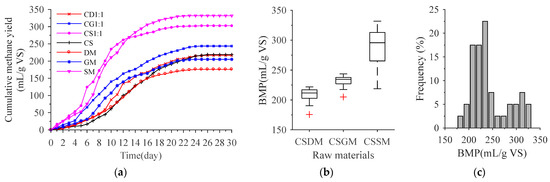
Figure 1.
BMP statistics of the anaerobic co-digestion feedstocks. (a) cumulative methane production of partial samples; (b) BMP boxplot of different sample categories; (c) BMP histogram of all samples. CD1:1, CG1:1 and CS1:1 represent the 1:1 mixtures of corn stover with dairy manure, goat manure and swine manure, respectively. CSDM, CSGM and CSSM represent the mixtures of corn stover with dairy manure, goat manure and swine manure, respectively.
BMP statistical data of co-AD feedstocks are shown in Table 2. The coefficient of variation is equal to the ratio of standard deviation to mean value, which can effectively eliminate the negative influence of differences of units or average values on the modeling performance [40]. As shown in Table 2, the coefficient of variation was 16.83% for the calibration set and 17.26% for the validation set, correspondingly, which showed that the large amount of variation among the BMP data was beneficial for constructing a robust model [24]. The result of the sample set partitioning ensured that the BMP data in the calibration set were consistent with those of the validation set and covered the validation set, which was suitable for development of the calibration model [44].
Table 2.
Biochemical methane potential statistical data of anaerobic co-digestion feedstocks.
Figure 2a shows that there are strong baseline offsets in the raw spectra. Figure 2b shows that the interference of baseline offsets and background noise in the spectral data is eliminated by preprocessing of MSC combined with SG smooth, thereby enhancing the resolution of spectral data, and raising the signal–noise ratio [45]. MSC can correct baseline offsets and spectral scattering, and SG smooth can effectively eliminate the influence of random noise on the modeling. For pretreated spectra, the low wavenumber region of 9000–4000 cm−1 has a stronger absorption peak, sharper waveform, better resolution and higher signal–noise ratio [46]. However, there are still plenty of redundant wavelengths in pretreated spectra, resulting in adverse influences on the accuracy and stability of the models. Therefore, it is necessary to perform CW selection to obtain key wavelengths for modeling [25].
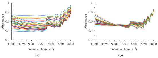
Figure 2.
Spectral data of the samples. (a,b) represent raw and pretreated spectra, respectively.
3.2. Selection of Characteristic Wavelengths
3.2.1. Characteristic Wavelengths Selected by SiPLS-GSA
When using SiPLS-GSA to select the CWs of the BMP, SiPLS was used to select the CSI first. To analyze the influence of the number of spectral interval divisions on the CWs selection and the modeling performance, whole spectra were partitioned into 15, 18, 23, 31, 37, 46 and 61 intervals, respectively, according to about 120, 100, 80, 60, 50, 40 and 30 wavelength variables contained in one interval. The RMSECV value corresponding to the combination of two to four intervals was calculated for each number of segmentation. By comparing RMSECV values of different interval combinations, the intervals (9 11 13 21) were taken as the CSI of BMP with 320 wavelength variables when spectra were divided into 23 intervals (gray shaded area in Figure 3).
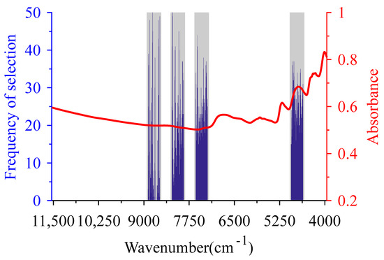
Figure 3.
Characteristic wavelengths of biochemical methane potential optimized by synergy iPLS—GSA (SiPLS-GSA). The gray bars are the characteristic spectra intervals selected by SiPLS, the blue histograms are the characteristic wavelengths selected by SiPLS-GSA, and the red line is the mean of the pretreated spectra.
When using GSA to further select CWs, the parameters of the algorithm were set as follows: CL of 320, population size of 110, initial temperature coefficient of 200, cooling coefficient of 0.95, evolutional algebra of 200, crossover probability of 0.7, mutation probability of 0.01, and disturbance bits of neighborhood solutions of 16. To resolve the uncertainty of the results selected by GSA, the procedure was executed 50 times to select wavelength variables in the CSIs of BMP. Then the corresponding RMSECV was calculated along with increasing the number of repeated selections. Wavelength variables corresponded to the number of repeated selections with the lowest RMSECV values being taken as the selected CWs of SiPLS-GSA. SiPLS-GSA was performed to obtain 285 wavelength variables as CWs with four repeated selections (blue histogram in Figure 3). Among the CWs selected by SiPLS-GSA, there was a higher frequency of selection corresponding to the second overtone region of carbon-containing groups such as C-H. The wavelengths in the second overtone and combination regions of N-H and C=O groups were selected more frequently. These C-H, N-H and C=O groups correspond to the carbohydrate, protein and lipid in organic matter [29,47]. This indicates that these three chemical components played a major role in the methane yield potential of co-AD [48].
3.2.2. Characteristic Wavelengths Selected by BiPLS-GSA
When BiPLS-GSA was used to select CWs of BMP, the same interval division scheme as SiPLS-GSA was adopted. BiPLS was used to select the combination of intervals for each number of segmentations first, and intervals (2 3 26 27 28 38 46 55 59) corresponding to the minimum RMSECV were taken as the CSI of BMP, with a total of 272 wavelength variables when spectra were divided into 61 intervals (gray shaded area in Figure 4).
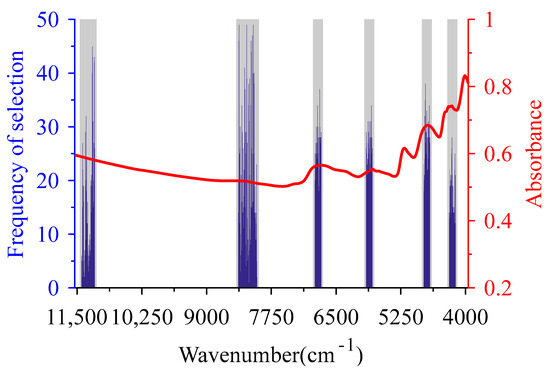
Figure 4.
Characteristic wavelengths of biochemical methane potential optimized by backward iPLS—GSA (BiPLS-GSA). The gray bars are the characteristic spectra intervals selected by BiPLS, the blue histograms are the characteristic wavelengths selected by BiPLS-GSA, and the red line is the mean of the pretreated spectra.
The number of wavelength variables (272) in CSI selected by BiPLS was taken as the CL, and 90 chromosomes were randomly generated to construct the initial population to execute the GSA for the further selection of CWs. The number of disturbance bits of neighborhood solutions was set to 14, and other parameters were consistent with SiPLS-GSA. After performing GSA 50 times, 260 wavelength variables with the number of repeated selections of four were selected as CWs of BiPLS-GSA (blue histogram in Figure 4). In the wavenumber of 11,100–11,400 cm−1 and 8000–8400 cm−1, there were wavelength variables with the higher frequency of selection corresponding to C-H group in CWs. While in other ranges, the wavelength variables corresponding to C=O, C-H and N-H groups were selected more frequently. These wavelength variables, which were selected more frequently, corresponded to the relevant groups in lignocellulose, protein and lipid components of the co-AD feedstocks.
3.2.3. Characteristic Wavelengths Selected by DGSA-PLS
GSA-iPLS adopted the same interval division scheme as SiPLS-GSA. For each number of intervals, the GSA-iPLS algorithm was executed 10 times, and the effective interval combinations were selected as the selected CSI according to RMSECV. When using GSA-iPLS to select the CSI, the number of interval partitions was taken as the CL, the population size was set to 100, and the number of disturbance bits of neighborhood solutions was set to one tenth of the CL (up rounding). Other parameters of GSA-iPLS were consistent with SiPLS-GSA. According to RMSECV, the intervals (8 14 16 17 21 26 33 34) were taken as the CSI of BMP with 398 wavelength variables when spectra were divided into 37 intervals (gray shaded area in Figure 5).
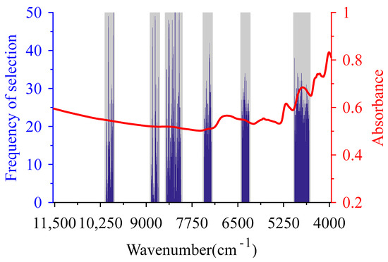
Figure 5.
Characteristic wavelengths of biochemical methane potential optimized by double GSA—partial least squares (DGSA-PLS). The gray bars are the characteristic spectra intervals selected by GSA-iPLS, the blue histograms are the characteristic wavelengths selected by DGSA-PLS, and the red line is the mean of the pretreated spectra.
DGSA-PLS took the number of wavelengths in the CSI selected by GSA-iPLS as CL, generated 160 chromosomes with CL of 398 to construct the initial population, and the number of perturbation bits of neighborhood solution was set to 20. Other initial parameters of the algorithm were consistent with SiPLS-iPLS. After performing GSA 50 times, 344 wavelength variables with eight repeated selections were selected as CWs of DGSA-PLS (blue histogram in Figure 5). There were 31 wavelength variables selected more than 35 times, which corresponded to second and third overtone regions of the C-H group, the overtones and combination band regions of N-H, and the combination band region of the C=O group.
3.2.4. Characteristic Wavelengths Selected by CARS-GSA
When using MCARS to select the CWs of BMP, CARS was executed 500 times first, and then the corresponding RMSECV was calculated along with increasing the number of repeated selections. The number of repeated selections with the lowest RMSECV corresponded to the wavelength variables as the selected BMP CWs of MCARS. MCARS was performed to obtain 383 alternative wavelengths, and 77 wavelength variables were selected as the CWs of MCARS corresponding to the number of repeated selections of 39 (Figure 6). This result indicates that MCARS can realize the effective compression of collinear wavelength variables while eliminating irrelevant wavelengths [40].
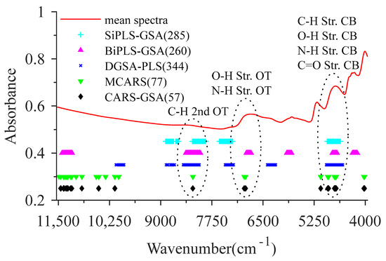
Figure 6.
Comparison of characteristic wavelengths selected by different variables selection methods. Str., OT and CB are short for stretch, overtone and combination, respectively.
When the CARS-GSA was used to select CWs of BMP, the number of CWs selected by MCARS was taken as the CL to randomly generate 40 chromosomes for the construction of the initial population. The number of perturbation bits of neighborhood solution was set to eight, and other parameters were consistent with SiPLS-GSA. After performing GSA for 50 times, 57 wavelength variables with the number of repeated selections of seven were selected as CWs of CARS-GSA (Figure 6). The CWs of MCAR and CARS-GSA mainly corresponded to the overtone region of the C-H group, the overtones and combination band regions of the N-H group, and the second, third overtones and combination band regions of the C=O group. CARS-GSA mainly eliminated wavelength variables of the third overtone region in CWs selected by MCARS.
For the CW selection algorithms proposed in the study, the repeatedly selected CWs, by four algorithms mainly located in the wavenumber ranges of 7750–8375 cm−1 and 4625–5250 cm−1. The CWs in 7750–8375 cm−1 relate to the C-H second overtone [23]. The absorption bands within 4625–5250 cm−1 are mainly attributed to the stretch and combination of the C-H, O-H, N-H and C=O groups [24]. In addition, the stretch first overtone of the O-H and N-H groups are indicated by spectral regions from 6500–7125 cm−1 [40]. Judging from the number of CWs selected by these four algorithms, CARS-GSA displayed the best capability in CWs selection for eliminating the uninformative wavelengths, which can improve the efficiency of the regression model.
3.3. Performance Analysis of Models
To investigate the modeling performance of different CW selection methods, the PLS regression models of BMP were established using CWs selected by SiPLS-GSA, BiPLS-GSA, DGSA-PLS and CARS-GSA, respectively. Predicted performances of the models were compared with those of the models constructed using whole wavelengths (denoted as Full-PLS) and CWs selected by SiPLS, BiPLS, CARS, and MCARS. Performance indicators of different models are shown in Table 3.
Table 3.
Evaluation indexes of regression models constructed by different wavelength selection methods.
Table 3 shows that the of models constructed using different wavelength selection algorithms is larger than 0.95, rRMSEP is less than 4.84, and their performances are superior to the Full-PLS model. This indicates that the redundant wavelengths of NIRS have a significant negative influence on the modeling accuracy [23]. It is necessary to eliminate the irrelevant wavelengths by the variables selection to establish a high-performance NIRS regression model [33]. It is important to note that the CARS-GSA algorithm acquired the best modeling performance with the of 0.984, RMSEP of 6.293 and rRMSEP of 2.600% for the validation set.
Figure 7 shows the scatter plots of the actual values and the predicted values for the CARS-GSA model. Overall, scatter points of the actual values and the predicted values were distributed along the 1:1 line, and the fit line coincided basically with the 1:1 line, indicating that the prediction precision of the model is excellent [49]. The results illustrate that the predicted model of BMP constructed by PLS combined with CARS-GSA can meet the requirement of rapid evaluation for methane production capacity of co-AD feedstocks.
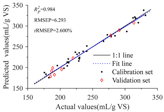
Figure 7.
Scatter diagrams of actual and predicted values for biochemical methane potential. : coefficient of determination for validation set, RMSEP: root mean square error for validation set, rRMSEP: relative root mean square error for validation set.
3.4. Discussion of the Description Results
For the CSI selection algorithms, the modeling performances of their selected wavelengths was ranked as GSA-iPLS > BiPLS > SiPLS. The reasons are as follows: Firstly, SiPLS searches two to four fixed number spectral intervals to obtain the key wavelengths, and it has a good advantage for the concentrated distribution of CWs [23]. Secondly, BiPLS eliminates the intervals one by one, and selects the combination intervals with the lowest RMSECV as the CSI. Compared with SiPLS, BiPLS is more suitable for solving the problem that CWs are widely distributed in the spectral region [25]. Thirdly, GSA-iPLS combines the partition strategy of iPLS with the search capability of GSA, and constructs the initial chromosome through the random combination of intervals [50]. Combining RMSECV with the temperature parameter to design the fitness function, GSA-iPLS completed the CSI selection through evolutionary operations. GSA-iPLS has greater random search capability and higher performance of wavelengths selection than SiPLS and BiPLS [51]. Finally, many degradable organic compounds (especially carbohydrates, lipids and crude proteins) in co-AD feedstocks have important effects on their methanogenic ability, and their corresponding groups are widely distributed throughout the spectral space [40]. Therefore, the predicted precision of the model constructed using CWs selected by GSA-iPLS outperformed models based on SiPLS and BiPLS.
Compared with the SiPLS, BiPLS and GSA-iPLS, CARS has a better modeling performance. It not only shows the high efficiency of CARS CWs selection, but also shows that the uninformative redundant wavelengths in CSI selected by SiPLS, BiPLS and GA-iPLS seriously affect the modeling performance [32]. It is necessary to use other algorithms to further eliminate the uninformative variables in CSI [45]. SiPLS-GSA, BiPLS-GSA and DGSA-PLS used GSA to select CWs from the preliminary results of SiPLS, BiPLS and GSA-iPLS, respectively. They can effectively eliminate the redundant wavelength variables in CSI selected by SiPLS, BiPLS and GSA-iPLS, thereby further improving the predicted performance of the regression model [31]. The main reason for this is that GSA can select the key wavelengths with high correlation to BMP, eliminate the variables with weak correlation and improve the regression accuracy of the model by selecting RMSECV as the target function [25]. Based on the powerful random search ability, GSA not only eliminates the weak correlation variables, but also solves the collinearity problem among wavelengths [24].
CARS constructs multiple subsets of CWs based on the RMSECV and the absolute value of the regression coefficient, which can effectively remove irrelevant and collinearity wavelength variables [52]. By taking repeatedly selected wavelengths as CWs after performing CARS for multiple times, MCARS not only resolves the inconsistency of results for CWs selected by CARS, but also effectively improves the modeling performance [40]. There may be some weak correlation wavelengths in the CWs selected by MCARS, which can be eliminated by the CARS-GSA. By the further selection of GSA, the number of CWs selected by CARS-GSA decreased to 57 and decreased by 25.97% compared with that of MCARS. The RMSEP of CARS-GSA model was 6.293, which decreased by 4.64% compared with that of MCARS. The rRMSEP decreased from 2.727% in MCARS model to 2.6000% in CARS-GSA model. These results indicate that CARS-GSA has an excellent performance in the CWs selection of BMP by combining MCARS with GSA.
For prediction accuracy of BMP regression model, the proposed NIRS models based on CARS-GSA is superior to the study results in the literature [27,29,36], such as an RMSEP of 37 and rRMSEP of 14.52% in the literature [35], RMSEP of 34 and rRMSEP of 11.83% in the literature [28], and RMSEP of 44 and rRMSEP of 7.42% in the literature [26]. The main reasons include two aspects: First, it is attributed to the efficiency of CW selection for CARS-GSA, and the other is that the sample type is relatively singular in this study. Aiming at the detection demand of BMP for co-AD with CS and LM as the substrate, mixtures of straw and manure were taken as feedstocks to construct the prediction model of BMP. It is beneficial to the construction of a special NIRS rapid detection system. However, the application scope of the model is limited. If the proposed CARS-GSA model is to be applied for the BMP detection of actual biogas engineering, it is necessary to extend the samples set to establish the more robust regression model. Especially, to detect BMP of other raw materials, such as chicken manure and rice straw, the model should be adjusted in addition to the new sample sampling, which is also the first task to establish a high availability NIRS detection model. Yao et al. [29] reported that the BMP of aquatic plants and algae was rapidly evaluated by the NIRS regression model, which was constructed by GA combined with a support vector machine. The predicted results, with an RMSEP of 16.61 and rRMSEP of 2.08%, indicate that the combination of CW selection and nonlinear modeling has good performance in modeling the NIRS regression model of BMP [33]. The combination of the proposed CW selection methods with nonlinear modeling methods, such as support vector machine and extreme learning machine, to establish a high-performance BMP prediction model also represents an important research direction in the future.
4. Conclusions
Quantitative models were developed with the NIRS data and BMP of co-AD feedstocks using four CWs selection algorithms, including SiPLS-GSA, BiPLS-GSA, DGSA-PLS and CARS-GSA. Among them, SiPLS-GSA, BiPLS-GSA, and DGSA-PLS realized the combination of characteristic spectral region selection and wavelengths for further optimization. CARS-GSA combined the CW preliminary positioning of MCARS with the further selection of GSA. By comparing the performance of regression models, it was found that the CARS-GSA model presented a better performance than other different models. For the CARS-GSA model, the RMSEP, rRMSEP and number of CWs were 6.293, 2.600% and 57, respectively, indicating that key variable selection by CARS-GSA could significantly improve the predicted performance of regression model. These results show that NIRS combined with CARS-GSA model can be successfully used for determination of the BMP for co-AD feedstocks.
Author Contributions
Conceptualization, C.L. and Y.S.; methodology, J.L.; validation, C.Z. and B.Z.; data curation, N.W. and J.S.; writing—original draft preparation, J.L. and C.Z.; writing—review and editing, C.L.; supervision, C.L. and Y.S. All authors have read and agreed to the published version of the manuscript.
Funding
This research was funded by the National Natural Science Foundation of China, grant number 52076034; the National Key R&D Program of China, grant number 2018YFE0206300-12; the Daqing Guidance Science and Technology Planned Project of China, grant number zd-2019-27; the Open Project Program of Key Laboratory of Technology and Model for Cyclic Utilization from Agricultural Resources, Ministry of Agriculture and Rural of China, grant number KLTMCUAR2020-2; the Scientific Research Foundation for Talent of Heilongjiang Bayi Agricultural University, grant number XDB202006 and the Postdoctoral Funding of Heilongjiang Province of China, grant number LBH-Z19087.
Institutional Review Board Statement
Not applicable.
Informed Consent Statement
Not applicable.
Data Availability Statement
Not applicable.
Acknowledgments
We would like to thank Zhengguang Chen at the College of Information and Electrical Engineering of Heilongjiang Bayi Agricultural University for his generosity to let us use their near infrared spectrometer for collecting spectral data.
Conflicts of Interest
The authors declare no conflict of interest.
References
- Sun, Y.; Zhang, Z.Z.; Sun, Y.M.; Yang, G.X. One-pot pyrolysis route to Fe−N-Doped carbon nanosheets with outstanding electrochemical performance as cathode materials for microbial fuel cell. Int. J. Agric. Biol. Eng. 2020, 13, 207–214. [Google Scholar] [CrossRef]
- Rekleitis, G.; Haralambous, K.; Loizidou, M.; Aravossis, K. Utilization of Agricultural and Livestock Waste in Anaerobic Digestion (A.D): Applying the Biorefinery Concept in a Circular Economy. Energies 2020, 13, 4428. [Google Scholar] [CrossRef]
- Yang, Y.; Ni, J.Q.; Zhu, W.; Xie, G. Life Cycle Assessment of Large-scale Compressed Bio-natural Gas Production in China: A Case Study on Manure Co-digestion with Corn Stover. Energies 2019, 12, 429. [Google Scholar] [CrossRef]
- Li, P.; Li, W.; Sun, M.; Xu, X.; Zhang, B.; Sun, Y. Evaluation of Biochemical Methane Potential and Kinetics on the Anaerobic Digestion of Vegetable Crop Residues. Energies 2019, 12, 26. [Google Scholar] [CrossRef]
- Qu, J.; Sun, Y.; Awasthi, M.K.; Liu, Y.; Xu, X.; Meng, X.; Zhang, H. Effect of different aerobic hydrolysis time on the anaerobic digestion characteristics and energy consumption analysis. Bioresour. Technol. 2021, 320, 124332. [Google Scholar] [CrossRef] [PubMed]
- Seruga, P.; Krzywonos, M.; Seruga, A.; Niedzwiecki, L.; Pawlak-Kruczek, H.; Urbanowska, A. Anaerobic Digestion Performance: Separate Collected vs. Mechanical Segregated Organic Fractions of Municipal Solid Waste as Feedstock. Energies 2020, 13, 3768. [Google Scholar] [CrossRef]
- Hamedani, S.R.; Villarini, M.; Colantoni, A.; Carlini, M.; Cecchini, M.; Santoro, F.; Pantaleo, A. Environmental and Economic Analysis of an Anaerobic Co-Digestion Power Plant Integrated with a Compost Plant. Energies 2020, 13, 2724. [Google Scholar] [CrossRef]
- Damtie, M.M.; Shin, J.; Jang, H.M.; Kim, Y.M. Synergistic Co-Digestion of Microalgae and Primary Sludge to Enhance Methane Yield from Temperature-Phased Anaerobic Digestion. Energies 2020, 13, 4547. [Google Scholar] [CrossRef]
- Rodrigues, R.P.; Rodrigues, D.P.; Klepacz-Smolka, A.; Martins, R.C.; Quina, M.J. Comparative analysis of methods and models for predicting biochemical methane potential of various organic substrates. Sci. Total Environ. 2019, 649, 1599–1608. [Google Scholar] [CrossRef]
- Mioduszewska, N.; Pilarska, A.A.; Pilarski, K.; Adamski, M. The Influence of the Process of Sugar Beet Storage on Its Biochemical Methane Potential. Energies 2020, 13, 5104. [Google Scholar] [CrossRef]
- Da Silva, C.; Astals, S.; Peces, M.; Campos, J.L.; Guerrero, L. Biochemical methane potential (BMP) tests: Reducing test time by early parameter estimation. Waste Manag. 2018, 71, 19–24. [Google Scholar] [CrossRef]
- Pilarski, K.; Pilarska, A.A.; Boniecki, P.; Niedbala, G.; Durczak, K.; Witaszek, K.; Mioduszewska, N.; Kowalik, I. The Efficiency of Industrial and Laboratory Anaerobic Digesters of Organic Substrates: The Use of the Biochemical Methane Potential Correction Coefficient. Energies 2020, 13, 1280. [Google Scholar] [CrossRef]
- Papirio, S.; Matassa, S.; Pirozzi, F.; Esposito, G. Anaerobic Co-Digestion of Cheese Whey and Industrial Hemp Residues Opens New Perspectives for the Valorization of Agri-Food Waste. Energies 2020, 13, 2820. [Google Scholar] [CrossRef]
- Yu, Q.; Sun, C.; Liu, R.; Yellezuome, D.; Zhu, X.; Bai, R.; Liu, M.; Sun, M. Anaerobic co-digestion of corn stover and chicken manure using continuous stirred tank reactor: The effect of biochar addition and urea pretreatment. Bioresour. Technol. 2021, 319, 124197. [Google Scholar] [CrossRef] [PubMed]
- Wei, L.; Qin, K.; Ding, J.; Xue, M.; Yang, C.; Jiang, J.; Zhao, Q. Optimization of the co-digestion of sewage sludge, maize straw and cow manure: Microbial responses and effect of fractional organic characteristics. Sci. Rep. 2019, 9, 2374. [Google Scholar] [CrossRef]
- Xu, Y.; Awasthi, M.K.; Li, P.; Meng, X.; Wang, Z. Comparative analysis of prediction models for methane potential based on spent edible fungus substrate. Bioresour. Technol. 2020, 317, 124052. [Google Scholar] [CrossRef] [PubMed]
- Khan, S.; Lu, F.; Jiang, Q.; Jiang, C.; Kashif, M.; Shen, P. Assessment of Multiple Anaerobic Co-Digestions and Related Microbial Community of Molasses with Rice-Alcohol Wastewater. Energies 2020, 13, 4866. [Google Scholar] [CrossRef]
- Thaemngoen, A.; Phuttaro, C.; Saritpongteeraka, K.; Leu, S.-Y.; Chaiprapat, S. Biochemical Methane Potential Assay Using Single Versus Dual Sludge Inocula and Gap in Energy Recovery from Napier Grass Digestion. Bioenergy Res. 2020, 13, 1321–1329. [Google Scholar] [CrossRef]
- Davidsson, Å.; Gruvberger, C.; Christensen, T.H.; Hansen, T.L.; Jansen, J.l.C. Methane yield in source-sorted organic fraction of municipal solid waste. Waste Manag. 2007, 27, 406–414. [Google Scholar] [CrossRef] [PubMed]
- Dong, J.; Dong, X.; Li, Y.; Peng, Y.; Chao, K.; Gao, C.; Tang, X. Identification of unfertilized duck eggs before hatching using visible/near infrared transmittance spectroscopy. Comput. Electron. Agric. 2019, 157, 471–478. [Google Scholar] [CrossRef]
- Li, J.; Zhang, M.; Dowell, F.; Wang, D.H. Rapid Determination of Acetic Acid, Furfural, and 5-Hydroxymethylfurfural in Biomass Hydrolysates Using Near-Infrared Spectroscopy. ACS Omega 2018, 3, 5355–5361. [Google Scholar] [CrossRef] [PubMed]
- Li, Y.; Altaner, C.M. Effects of variable selection and processing of NIR and ATR-IR spectra on the prediction of extractive content in Eucalyptus bosistoana heartwood. Spectrochim. Acta A 2019, 213, 111–117. [Google Scholar] [CrossRef]
- Liu, J.; Chu, X.; Wang, Z.; Xu, Y.; Li, W.; Sun, Y. Optimization of Characteristic Wavelength Variables of Near Infrared Spectroscopy for Detecting Contents of Cellulose and Hemicellulose in Corn Stover. Spectrosc. Spect. Anal. 2019, 39, 743–750. [Google Scholar] [CrossRef]
- Liu, J.; Jin, S.; Bao, C.; Sun, Y.; Li, W. Rapid determination of lignocellulose in corn stover based on near-infrared reflectance spectroscopy and chemometrics methods. Bioresour. Technol. 2021, 321, 124449. [Google Scholar] [CrossRef] [PubMed]
- Liu, J.; Li, N.; Zhen, F.; Xu, Y.; Li, W.; Sun, Y. Rapid detection of carbon-nitrogen ratio for anaerobic fermentation feedstocks using near-infrared spectroscopy combined with BiPLS and GSA. Appl. Optics 2019, 58, 5090–5097. [Google Scholar] [CrossRef]
- Fitamo, T.; Triolo, J.M.; Boldrin, A.; Scheutz, C. Rapid biochemical methane potential prediction of urban organic waste with near-infrared reflectance spectroscopy. Water Res. 2017, 119, 242–251. [Google Scholar] [CrossRef]
- Godin, B.; Mayer, F.; Agneessens, R.; Gerin, P.; Dardenne, P.; Delfosse, P.; Delcarte, J. Biochemical methane potential prediction of plant biomasses: Comparing chemical composition versus near infrared methods and linear versus non-linear models. Bioresour. Technol. 2015, 175, 382–390. [Google Scholar] [CrossRef]
- Mortreuil, P.; Baggio, S.; Lagnet, C.; Schraauwers, B.; Monlau, F. Fast prediction of organic wastes methane potential by near infrared reflectance spectroscopy: A successful tool for farm-scale biogas plant monitoring. Waste Manag. Res. 2018, 36, 800–809. [Google Scholar] [CrossRef]
- Yao, Y.; Shen, X.; Qiu, Q.; Wang, J.; Cai, J.; Zeng, J.; Lang, X. Predicting the Biochemical Methane Potential of Organic Waste with Near-Infrared Reflectance Spectroscopy Based on GA-SVM. Spectrosc. Spect. Anal. 2020, 40, 1857–1861. [Google Scholar] [CrossRef]
- Ward, A.J. Near-Infrared Spectroscopy for Determination of the Biochemical Methane Potential: State of the Art. Chem. Eng. Technol. 2016, 39, 611–619. [Google Scholar] [CrossRef]
- Yun, Y.H.; Bin, J.; Liu, D.L.; Xu, L.; Yan, T.L.; Cao, D.S.; Xu, Q.S. A hybrid variable selection strategy based on continuous shrinkage of variable space in multivariate calibration. Anal. Chim. Acta 2019, 1058, 58–69. [Google Scholar] [CrossRef]
- Chen, Y.; Ma, H.; Zhang, Q.; Zhang, S.; Chen, M.; Wu, Y. Comparison of several variable selection methods for quantitative analysis and monitoring of the Yangxinshi tablet process using near-infrared spectroscopy. Infrared Phys. Technol. 2020, 105, 103188. [Google Scholar] [CrossRef]
- Ren, G.; Ning, J.; Zhang, Z. Multi-variable selection strategy based on near-infrared spectra for the rapid description of dianhong black tea quality. Spectrochim. Acta A 2021, 245, 118918. [Google Scholar] [CrossRef] [PubMed]
- Huang, J.; Ren, G.; Sun, Y.; Jin, S.; Li, L.; Wang, Y.; Ning, J.; Zhang, Z. Qualitative discrimination of Chinese dianhong black tea grades based on a handheld spectroscopy system coupled with chemometrics. Food Sci. Nutr. 2020, 8, 2015–2024. [Google Scholar] [CrossRef] [PubMed]
- Triolo, J.M.; Ward, A.J.; Pedersen, L.; Løkke, M.M.; Qu, H.; Sommer, S.G. Near Infrared Reflectance Spectroscopy (NIRS) for rapid determination of biochemical methane potential of plant biomass. Appl. Energ. 2014, 116, 52–57. [Google Scholar] [CrossRef]
- Zhang, B.; Li, W.; Xu, X.; Li, P.; Li, N.; Zhang, H.; Sun, Y. Effect of Aerobic Hydrolysis on Anaerobic Fermentation Characteristics of Various Parts of Corn Stover and the Scum Layer. Energies 2019, 12, 381. [Google Scholar] [CrossRef]
- Nørgaard, L.; Saudland, A.; Wagner, J.; Nielsen, J.P.; Munck, L.; Engelsen, S.B. Interval Partial Least-Squares Regression (iPLS): A Comparative Chemometric Study with an Example from Near-Infrared Spectroscopy. Appl. Spectrosc. 2000, 54, 413–419. [Google Scholar] [CrossRef]
- Leardi, R.; Norgaard, L. Sequential application of backward interval partial least squares and genetic of relevant spectral regions. J. Chemometrics 2004, 18, 486–497. [Google Scholar] [CrossRef]
- Li, H.D.; Liang, Y.Z.; Xu, Q.S.; Cao, D.S. Key wavelengths screening using competitive adaptive reweighted sampling method for multivariate calibration. Anal. Chim. Acta 2009, 648, 77–84. [Google Scholar] [CrossRef]
- Yang, G.; Li, Y.; Zhen, F.; Xu, Y.; Liu, J.; Li, N.; Sun, Y.; Luo, L.; Wang, M.; Zhang, L. Biochemical methane potential prediction for mixed feedstocks of straw and manure in anaerobic co-digestion. Bioresour. Technol. 2021, 326, 124745. [Google Scholar] [CrossRef] [PubMed]
- Gaballah, E.S.; Abomohra, A.E.-F.; Xu, C.; Elsayed, M.; Abdelkader, T.K.; Lin, J.; Yuan, Q. Enhancement of biogas production from rape straw using different co-pretreatment techniques and anaerobic co-digestion with cattle manure. Bioresour. Technol. 2020, 309, 123311. [Google Scholar] [CrossRef]
- Wang, Y.; Zhang, J.; Li, Y.; Jia, S.; Song, Y.; Sun, Y.; Zheng, Z.; Yu, J.; Cui, Z.; Han, Y.; et al. Methane production from the co-digestion of pig manure and corn stover with the addition of cucumber residue: Role of the total solids content and feedstock-to-inoculum ratio. Bioresour. Technol. 2020, 306, 123172. [Google Scholar] [CrossRef]
- Xue, J.; Yang, Z.; Han, L.; Liu, Y.; Liu, Y.; Zhou, C. On-line measurement of proximates and lignocellulose components of corn stover using NIRS. Appl. Energ. 2015, 137, 18–25. [Google Scholar] [CrossRef]
- Liang, L.; Wei, L.; Fang, G.; Xu, F.; Deng, Y.; Shen, K.; Tian, Q.; Wu, T.; Zhu, B. Prediction of holocellulose and lignin content of pulp wood feedstock using near infrared spectroscopy and variable selection. Spectrochim. Acta A 2019, 225, 117515. [Google Scholar] [CrossRef] [PubMed]
- Cheng, J.; Chen, Z. Wavelength Selection of Near-Infrared Spectra Based on Improved SiPLS-Random Frog Algorithm. Spectrosc. Spect. Anal. 2020, 40, 3451–3456. [Google Scholar] [CrossRef]
- Xie, H.; Chen, Z.G. Application of Genetic Simulated Annealing Algorithm in Detection of Corn Straw Cellulose. Chin. J. Anal. Chem. 2019, 47, 1987–1994. [Google Scholar] [CrossRef]
- Charnier, C.; Latrille, E.; Roger, J.M.; Miroux, J.; Steyer, J.P. Near-Infrared Spectrum Analysis to Determine Relationships between Biochemical Composition and Anaerobic Digestion Performances. Chem. Eng. Technol. 2018, 41, 727–738. [Google Scholar] [CrossRef]
- Raposo, F.; Borja, R.; Ibelli-Bianco, C. Predictive regression models for biochemical methane potential tests of biomass samples: Pitfalls and challenges of laboratory measurements. Renew. Sustain. Energ. Rev. 2020, 127, 109890. [Google Scholar] [CrossRef]
- Guo, Q.; Nie, L.; Li, L.; Zang, H. Estimation of the critical quality attributes for hydroxypropyl methylcellulose with near-infrared spectroscopy and chemometrics. Spectrochim. Acta A 2017, 177, 158–163. [Google Scholar] [CrossRef] [PubMed]
- Zhao, J.; Tian, G.; Qiu, Y.; Qu, H. Rapid quantification of active pharmaceutical ingredient for sugar-free Yangwei granules in commercial production using FT-NIR spectroscopy based on machine learning techniques. Spectrochim. Acta A 2020, 245, 118878. [Google Scholar] [CrossRef]
- Yang, M.; Xu, D.; Chen, S.; Li, H.; Shi, Z. Evaluation of Machine Learning Approaches to Predict Soil Organic Matter and pH Using vis-NIR Spectra. Sensors 2019, 19, 263. [Google Scholar] [CrossRef] [PubMed]
- Weng, S.; Guo, B.; Tang, P.; Yin, X.; Pan, F.; Zhao, J.; Huang, L.; Zhang, D. Rapid detection of adulteration of minced beef using Vis/NIR reflectance spectroscopy with multivariate methods. Spectrochim. Acta A 2020, 230, 118005. [Google Scholar] [CrossRef] [PubMed]
Publisher’s Note: MDPI stays neutral with regard to jurisdictional claims in published maps and institutional affiliations. |
© 2021 by the authors. Licensee MDPI, Basel, Switzerland. This article is an open access article distributed under the terms and conditions of the Creative Commons Attribution (CC BY) license (http://creativecommons.org/licenses/by/4.0/).