Article

A Long Short-Term Memory Neural Network for the Low-Cost Prediction of Soot Concentration in a Time-Dependent Flame

Department of Mechanical and Industrial Engineering, Ryerson University, Toronto, ON M5B 2K3, Canada
*
Author to whom correspondence should be addressed.
Energies 2021, 14(5), 1394; https://doi.org/10.3390/en14051394
Submission received: 28 January 2021 / Revised: 16 February 2021 / Accepted: 27 February 2021 / Published: 3 March 2021
(This article belongs to the Special Issue Machine Learning Applications to Combustion Engines)

Abstract

:
Particulate matter (soot) emissions from combustion processes have damaging health and environmental effects. Numerical techniques with varying levels of accuracy and computational time have been developed to model soot formation in flames. High-fidelity soot models come with a significant computational cost and as a result, accurate soot modelling becomes numerically prohibitive for simulations of industrial combustion devices. In the present study, an accurate and computationally inexpensive soot-estimating tool has been developed using a long short-term memory (LSTM) neural network. The LSTM network is used to estimate the soot volume fraction ( f v ) in a time-varying, laminar, ethylene/air coflow diffusion flame with 20 Hz periodic fluctuation on the fuel velocity and a 50% amplitude of modulation. The LSTM neural network is trained using data from CFD, where the network inputs are gas properties that are known to impact soot formation (such as temperature) and the network output is f v . The LSTM is shown to give accurate estimations of f v , achieving an average error (relative to CFD) in the peak f v of approximately 30% for the training data and 22% for the test data, all in a computational time that is orders-of-magnitude less than that of high-fidelity CFD modelling. The neural network approach shows great potential to be applied in industrial applications because it can accurately estimate the soot characteristics without the need to solve the soot-related terms and equations.

1. Introduction

Soot emission from combustion systems can be a substantial threat to human health and to the environment [1]. Increasingly strict emissions regulations (e.g., the EURO 6 standard) are emerging to combat the negative effects of soot emission, leaving designers with two major avenues-experiments and numerical simulations—to model, understand, and reduce soot formation in combustion systems. A general advance in the knowledge and capabilities of the soot modelling community has allowed a push past empirical or semi-empirical soot models and into robust soot models inspired by the underlying physico-chemical processes of soot formation. These high-fidelity soot models (e.g., [2]) generally give detailed consideration to phenomena such as nucleation from polycyclic aromatic hydrocarbons (PAHs), PAH condensation, physical coagulation, surface growth by the hydrogen-abstraction-carbon-addition (HACA) mechanism, oxidation, and oxidation-induced fragmentation on soot formation and evolution. Recent advancements, including reversible nucleation [3] and condensation [4,5] models, detailed models to track soot maturity [6] and internal structure [7], and the consideration of chemical bond formation in the inception process [8], have greatly advanced high-fidelity CFD models. However, many knowledge gaps, particularly in the inception step [9], still remain in CFD soot modelling.
In general, the consideration of the above-mentioned phenomena is extremely time-consuming, especially as the sub-models become more detailed and physically realistic. The cumbersome nature of high-fidelity models has pushed many industries to use semi-empirical soot models which, although faster, may sacrifice a good deal of accuracy compared to their high-fidelity counterparts (relative errors of 1–2 orders of magnitude in soot volume fraction prediction [10,11,12,13]). To circumvent the clash between accuracy and cost in traditional soot modelling methods, a novel computational concept called the “soot estimator” has been recently introduced [14,15,16,17]. In the soot estimator concept, only a validated combustion model is needed, and the soot characteristics are estimated without solving the soot-related terms and equations. In a practical context, relieving the need to calculate the soot-related terms will save valuable computational time and may greatly facilitate the design process in industry. The soot estimator approach is essentially a soot post-processing tool that is linked to computational fluid dynamics (CFD) simulations of combustion environments. In this approach, gas-related properties such as temperature and species mass fractions are obtained from the solution of gas-phase conservation equations (mass, momentum, energy and species mass fractions). The gas properties are then used to estimate the soot characteristics, such as soot volume fraction f v :
f v ( t ) = f ( T ( t ) , Y i ( t ) , P ( t ) , ) ,
where T is the gas temperature, Y i is the mass fraction of species i, P is the pressure, and t is the time. Bozorgzadeh [14], who first introduced the soot estimator concept in 2014, reasoned that the larger timescales of soot formation and destruction relative to those of flow and gas-phase chemistry implied that the residence time of the soot particles should be considered. Therefore, Bozorgzadeh suggested that local instantaneous soot properties such as soot volume fraction should be a function of the temporal (time-integrated) histories of the above-mentioned gas-related variables. Temporal integration was performed over the pathlines of the soot particles, which were extracted from CFD using the Lagrangian approach. Equation (1) then becomes:
f v ( t ) = f ( T h ( t ) , Y i , h ( t ) , P h ( t ) , ) ,
where the subscript h represents the time-integrated history of the corresponding variable. To keep true to the premise of a low-cost (yet accurate) soot estimator, it was necessary to select key variables to track, so as to limit the dimensionality and reduce computational cost. For example, Equation (3) below:
f v ( t ) f ( T h ( t ) , M F h ( t ) , H 2 , h ( t ) ) ,
would attempt to relate the soot volume fraction in the flame to selected gas parameters, namely: the histories of temperature, mixture fraction, and H2 concentration, respectively. The relationship between the soot characteristics and the gas-related parameters (i.e., the function f in Equation (3)) is central to the soot estimator concept and was a major focus in previous developments [14,15,16,17].
In [14,15,16,17], previous versions of the soot estimator were used to estimate the soot characteristics of steady coflow laminar diffusion flames at atmospheric pressure. In these studies, the CFD code called CoFlame [2] was used to generate the required data, i.e., the gas parameters such as temperature and species concentrations. In the work of Bozorgzadeh [14], polynomial functions were used to link the CFD results to the desired soot characteristic. At first, soot concentration was related to temperature history, and later to both temperature and acetylene histories. The author found that in both cases, polynomial functions were not able to reproduce the soot concentration accurately. The addition of other parameters such as 0 2 , h (which can be considered an indicator of oxidation and soot reduction) helped increase the estimation accuracy. However, this increase in the dimensionality of the function was accompanied by a steep increase in computational cost, leading to a new estimation approach in [15,16]—tabulating the relationships between the histories of gas-related variables and the soot concentration.
To generate the lookup tables (also referred to as the libraries), Alexander et al. [15] and Zimmer et al. [16] grouped the histories of the gas-related variables into bins. Each variable is a “dimension” of the table and each dimension has a certain number of bins. In [16], 4D tables (i.e., f v and the histories of three variables) were generated for steady laminar diffusion flames using 300 bins in each dimension. In these studies, the number of dimensions and the number of bins were very sensitive parameters. An increase in the number of dimensions or bins could result in a disproportionate increase in memory requirement and computational time. In addition, the variable selection had a large impact on the results. For example, Zimmer et al. [16] showed that changing the variables in the table from [ T h ( t ) , M F h ( t ) , H 2 , h ( t ) ] to [ T h ( t ) , M F h ( t ), O 2 , h ( t ) ] increased the error (measured relative to model predictions) in f v estimation by around 57%. Furthermore, the tabular scheme may not scale well to more complex problems. As originally discussed by Zimmer et al. [16], the dimensionality issues become more significant when the tool is extended to transient and turbulent diffusion flames, where the the amount of required data can be much larger than in steady laminar flame simulations.
The above-mentioned limitations inspired the deep learning approach recently developed by Jadidi et al. [17]. As in many fields, the use of deep learning and artificial neural networks (ANN) is becoming increasingly pervasive in combustion research. As far back as the mid 1990s, Christo et al. [18,19] used an ANN to estimate the reaction chemistry in turbulent flames. Christo et al. [18] found that the ANN can yield predictions of “reasonable” accuracy (absolute errors on the order of 10 7 ) in a computational time that was one order of magnitude less than the direct integration approach. The authors went on to stress that the accuracy of the ANN model was strongly dependent on the selection of the training data sets and that a broad, dynamic range of training samples can improve the accuracy and generality of the ANN. In the recent work of Ranade et al. [20], an ANN was used to develop a computationally inexpensive chemical kinetics model. As the authors explain, an ANN may be applied to relieve some of the complexity and computational requirements inherent in the development of a detailed chemistry model. In [20], a shallow ANN was used to fit temporal profiles of fuel fragments, and a deep ANN was used to predict chemical reaction rates during pyrolysis. The ANN approach showed reasonable agreement with the detailed chemistry results.
These works, and a selection of others (e.g., [21,22,23,24,25,26,27]), show that an ANN is a versatile tool that can be used to reduce computational time at the expense of a minor decrease in accuracy (compared to traditional tools). As such, a handful of recent works have applied ANNs to the field of soot estimation [17,28,29,30,31]. The work of Talebi-Moghaddam et al. [28] used an ANN to efficiently and accurately estimate the light scattering kernel that is used in experiments to infer the morphological characteristics of soot particles. Furthermore, a handful of studies [29,30,31] have used ANNs to couple engine operational parameters such as crank angle or fuel consumption to the soot emissions from engines. In [29], a shallow (1 hidden layer) multilayer perceptron ANN was used to predict the soot, C O 2 , and NO x emissions from a direct injection diesel engine. The study used the CFD-computed quantities of crank angle, temperature, pressure, liquid mass evaporated, equivalence ratio, and O 2 concentration as input to the ANN. The optimal ANN architecture achieved a mean squared error on the order of 10 4 for the soot, C O 2 , and NO x predictions (soot, C O 2 , and NO x predictions on the order of 10 3 , 10 2 , and 10 4 , respectively). The study of Ghazikhani and Mirzaii [30] used a shallow multilayer perceptron ANN to predict the soot density in the exhaust of a turbo-charged diesel engine. Six experimentally measured parameters (inlet manifold pressure, inlet manifold temperature, inlet air mass flow rate, fuel consumption, engine torque, and speed) were used as input to the neural network and the network achieved a mean absolute percent error of about 6% relative to experimental measurements.
The study of Alcan et al. [31] used a gated recurrent unit (GRU) neural network (which is similar to the long short-term memory neural network used in the present study) to estimate the soot emission from a diesel engine. The network inputs were experimentally determined and consisted of engine speed, total injected fuel quantity, main start of injection, rail pressure, and intake oxygen ratio. The results showed accuracies of 77% on the training data and 57% on the validation data. Finally, the study of Yang et al. [32] used a long short-term memory (LSTM) neural network—the same type of neural network used in the present study—to predict NO x emissions from coal burners. The study used 35 experimentally measured parameters that are relevant to NO x emissions from a coal burner as input to the LSTM. The authors concluded that the LSTM could give reasonably accurate NO x estimations, with 54% of the test data showing a relative error less than 0.01 and an overall root mean squared error of 2.271 (for NO x emission levels on the order of 10 2 ). While these studies have laid the groundwork for the present objective of devising a more broadly applicable ANN system of soot prediction, each of them considers one or few specific operating configurations. By contrast, the present work is a step toward developing an ANN to predict soot characteristics in a broad range of conditions and configurations.
In the recent work of Jadidi et al. [17], the authors used a multilayer perceptron ANN to pair the combustion conditions (the input) to the resulting soot characteristics (the target). As in the previous studies [14,15,16], CoFlame [2] was used to generate the flame data. After generation of the combustion data, the Lagrangian histories of soot-containing fluid parcels were calculated using the approach developed by Zimmer et al. [16]. Subsequently, eight parameters, selected due to their significant influence on soot formation, were fed to the network as the input dataset. These eight parameters were the temperature history ( T h ), mixture fraction history ( M F h ), oxygen history ( O 2 , h ), carbon monoxide history ( C O h ), carbon dioxide history ( C O 2 , h ), hydrogen history ( H 2 , h ), hydroxide history ( O H h ), and acetylene history ( C 2 H 2 h ). The soot volume fraction was the output of the network. Overall, the ANN approach of Jadidi et al. [17] was successful; the authors found that the network could estimate the shape of the soot regions as well as the values of soot concentration very well and with low computational cost. Additionally, the use of eight parameters highlighted the network’s ability to handle a high-dimensional input, providing a degree of flexibility that was not present in the previous studies [14,15,16] (i.e., the amount of dimensions can be changed depending on the accuracy and computational requirements).
While the multilayer perceptron ANN of [17] was applicable to a steady flame, there exist more complex and versatile neural network architectures (namely, recurrent neural networks or RNNs) that were designed specially for time-series data. Therefore, as practical combustion devices are inherently transient, the main objective of the current study is to extend the capability of the ANN-based soot estimator to time-dependent flames. Ultimately, the aim of this and future works is to develop the ANN-based soot estimator into a tool for industry end use that quickly and accurately estimates soot characteristics without requiring a large amount of computing resources. In the present study, a time-varying, laminar, ethylene/air coflow diffusion flame with 20 Hz periodic fluctuation on the fuel velocity and a 50% amplitude of modulation, the same as [33], is considered. An LSTM neural network, a type of RNN, will be used for the soot estimator tool. The numerical simulation of this flame, which was performed and validated by Dworkin et al. [33], is used as the LSTM neural network’s training and testing data. The use of an LSTM neural network for soot estimation is, to the authors’ knowledge, novel. Further novelty (relative to the above-mentioned ANN/soot studies) of the present work (as well as [17]) stems from the soot estimator tool being trained using a detailed CFD model. The ANN is trained using inputs that are fundamental to the soot inception, growth, and oxidation processes (such as O H and C 2 H 2 mass fractions), thereby training the ANN to recognize the foundational relationships between the gas phase and soot concentration.
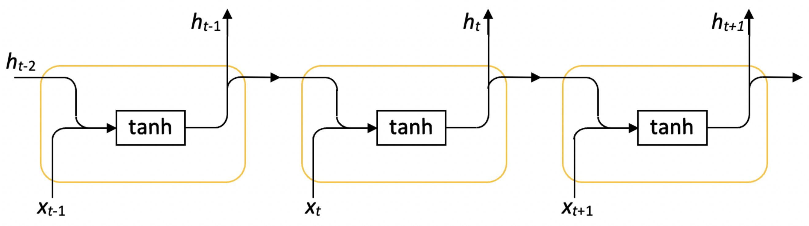
An LSTM network is better-suited for transient flame predictions, compared to a multilayer perceptron ANN, due to the LSTM’s inherent ability to learn long-term temporal interdependencies between time steps of sequential data [32]. Furthermore, the use of an LSTM will eliminate assumptions and potential sources of error that were present in the previous works. In the previous implementations of the soot estimator tool [16,17], it was necessary to (1) calculate the pathlines of soot containing fluid parcels, (2) compute the history of a given variable (i.e., the time integration of the variable over its lifetime), and (3) perform linear interpolation to distribute the estimated f v values from the pathlines onto the r-z coordinate system [17]. In the present work, the gas-related variables computed by CFD can be fed directly to the LSTM (eliminating the need for steps 1–3), since the LSTM inherently considers time-dependence. By design, the LSTM learns the temporal relationships between the input and output data. Therefore, the widely varying characteristic time scales between combustion kinetics and soot formation are accounted for without issue. Previously, step 2 assumed, without validation, the simplest form of the time integration, i.e., it assumed that the history of a variable had a linear relationship with the variable itself, with an implied weighting function of unity. The use of the LSTM network eliminates the need for that assumption and the potential error associated with it.
In the following section, the CFD simulations, flame conditions, and LSTM fundamentals are explained. Subsequently, the data preprocessing, network architecture, and the LSTM’s performance and error relative to CFD are discussed.

2. Methodology

2.1. CFD Simulations and Flame Conditions

In the present study, the numerical simulation of Dworkin et al. [33] is used to train and test the neural network. In the numerical study of Dworkin et al. [33], a high-fidelity, parallelized CFD code was used to solve the time-dependent, 2D axisymmetric equations for the conservation of vorticity, velocity, chemical species, energy, and soot. The CFD employed a sectional soot model with 20 logarithmically spaced sections. The soot model considers inception, coalescence, surface growth, and oxidation. Briefly, the following boundary conditions were applied: a symmetry condition at the centerline of the diffusion flame (r = 0), a free slip condition (normal component of axial velocity set to 0) at the far-radial boundary ( r ), a zero gradient condition at the axial outlet ( z ), and velocity inlet conditions for fuel and air at the burner (z = 0). Full expressions for the governing equations and the boundary conditions are given in the original study [33].
The flame, originally considered in [33], is a transient laminar sooting ethylene/air coflow diffusion flame with a periodic fluctuation of 20 Hz on the fuel velocity. The fuel was a mixture with a mass fraction of 0.32 for ethylene and 0.68 for nitrogen. Different amplitudes of modulation (30%, 50%, 70%, and 90%) were imposed on the fuel velocity in [33], although only the 50% case was taken for the present study since those results were validated against experimental data. The equation for the inlet fuel velocity is:
v z , i n l e t , f u e l = 2 v z , a v g ( 1 + α sin 2 π f t ) 1 r r 1 2 ,
where v z , a v g is the average spatial and temporal fuel inlet velocity (35 cm/s), r is the radial value, r 1 is the inner radius of the fuel tube, α is the amplitude of modulation, and f is the frequency of modulation.
It is pertinent to mention here that, as input to the soot estimator, any errors in the CFD modelling (relative to experiment) would propagate into the soot estimator. While the error between CFD and experiment varies depending on the complexity of the flame and CFD submodels, most CFD models are able to capture the trends and gradients of soot characteristics very well (e.g., see [2,5,34,35]). As the soot estimator tool is geared towards industry design use, the ability to estimate trends in soot emissions is a valuable trait. Moreover, as CFD simulations become more accurate, the propagation of error between CFD and the LSTM will be reduced.

2.2. LSTM Theory

Before LSTM networks are discussed in detail, a brief review of ANNs is warranted. An ANN is a computational tool that is used to predict an output when given input data. The network has layers of “neurons” (also referred to as nodes) that have weights and biases. Input data is passed to a neuron, multiplied by the weight, the bias is added on, and then the result is passed through an activation function (for example, the hyperbolic tangent function). The result of the activation function is passed to the nodes in the next layer, where the process continues until the final layer of nodes in the network (the output layer). This output is the prediction of the neural network.
In the current context, the input data is computed CFD data, such as temperature and gas composition, and the output is the soot volume fraction in the flame. A training data set is assembled, where the inputs and outputs are known. The prediction from the network is compared to the expected “answer” in the training data and the weights and biases are updated such that the difference between the network’s prediction and the expected answer is minimized. This process is repeated for a specified number of epochs, where an epoch is one pass through the whole training data set. After the network is trained, it is ready to be applied to a new problem and predict an output without needing to have the answer pre-computed. Neural networks are at the heart of deep learning and have facilitated sensational progress in fields such as finance, medicine, natural language processing, and autonomous vehicle operation [36]. Further detail on the theory and operation behind fully connected (or dense) neural networks may be found in [17].
An LSTM network [37] is an advanced neural network architecture that is used in problems with sequential or time series input data such as in fluid mechanics and combustion. LSTM networks were based on the recurrent neural network (RNN) architecture and were designed to solve the stability issues inherent to traditional RNNs [38]. An RNN is a broad class of neural networks where the output of the hidden layer (the layer of nodes where weights and biases are applied) is returned back into the network [38]. Figure 1 shows an illustration of the general RNN concept. In Figure 1, the input at time step t 1 (i.e., x t 1 ) is fed to a neuron with a t a n h activation function, and the output ( h t 1 ) from that time step is fed as input (along with x t ) to the subsequent node. This procedure allows the network to “remember” information from previous time steps and make predictions in an environment where knowledge of prior information is necessary (for example, predicting the next word in a sentence). This method effectively permits time-history consideration that is necessary for soot prediction, especially given the varying timescales of soot growth and combustion kinetics. However, the self-feedback of the basic RNN model can lead to an amplification problem, where the gradients computed during process of updating the weights and biases can either explode or vanish over many time steps (the so-called exploding or vanishing gradient problems) [32,38].
LSTM networks retain the basic concept of RNNs, but use a set of gates to control the passage of information between neurons. An LSTM layer is composed of “memory cells” which consist of the following 4 components: a forget ( f t ), input ( i t ), and output gate ( o t ), as well as an input node ( C ˜ t ) [32,38]. The structure of an LSTM memory cell is shown below in Figure 2, where the squares represent trainable nodes (i.e., they have weights and biases) and the circles represent pointwise mathematical operations. The writing inside the squares and circles shows the activation function and the mathematical operation, respectively. The 2 activation functions, sigmoid (denoted by σ ) and hyperbolic tangent (denoted by t a n h ) are defined below in Equations (5) and (6) [32].
σ ( z ) = 1 1 + e z ,
t a n h ( z ) = e z e z e z + e z .
Within the memory cell, the input gate controls how much of the input the network should retain (i.e., it “gates” the input) [38]. The sigmoid activation function is used because it ranges from 0 to 1, where 0 would denote that none of the input is retained and 1 would denote that all of the input is retained. The outputs of the input gate and the input node undergo a pointwise multiplication and the result is then added to the internal state of the memory cell. The internal state can be thought of as the cell’s memory because information from the previous cells are stored there (from the input C t 1 ). This retention of information from previous nodes is the key element to LSTM networks and allows them to work well with data where patterns or important information is spread across large gaps [38]. The forget gate also interacts with the internal state, and it determines how much of the internal state to neglect [38]. In essence, the forget gate drops part of the cell’s memory after seeing the current input. The input gate and input node are multiplied and after the addition of that quantity to the internal state, the hyperbolic tangent function is used to scale the result between −1 and 1. The scaled result is multiplied by the result of the output gate, which controls how much of the internal state to send to the next cell [38].
In Figure 2, the input to the memory cell, x t , is from the input data set. Vertically, the cell outputs h t to the corresponding cell in the next LSTM layer. Horizontally, C t and h t send the cell’s internal state and output, respectively, to the next LSTM cell in the current layer. The mathematical expressions for the LSTM memory cell are listed below in Equations (7)–(12) [38].
f t = σ ( W f x x t + W f h h t 1 + b f ) ,
i t = σ ( W i x x t + W i h h t 1 + b i ) ,
C ˜ t = t a n h ( W C ˜ x x t + W C ˜ h h t 1 + b C ˜ ) ,
o t = σ ( W o x x t + W o h h t 1 + b o ) ,
C t = f t · C t 1 + i t · C ˜ t ,
h t = t a n h ( C t ) · o t ,
where W j k is the weight vector for gate j and connection k (i.e., either the input connection x or the recurrent connection h), b j is the bias for gate j, σ and t a n h are the sigmoid and hyperbolic tangent functions defined above, and · represents the pointwise multiplication of vectors [38].

2.3. LSTM Application

As mentioned above, the input to the soot estimator is a selection of gas-related properties and the output of the soot estimator is the soot volume fraction f v . In this study, the gas-phase temperature as well as the mass fractions of C 2 H 4 , O 2 , O H , H 2 , C 2 H 2 with respect to time, are the inputs to the LSTM neural network. Note that the LSTM does not receive any soot-related terms as input, which can save a large amount of computational time. The merit of the soot estimator approach rests in the fact that, for a well-trained neural network, the savings in computational time do not sacrifice significant accuracy compared to CFD predictions. In fact, the results of [17] have shown that a neural network can predict soot volume fraction (given non-soot related terms as inputs) to within 20% of a high-fidelity CFD model such as CoFlame [2]. Here, it is also worth reiterating the scope and application of this tool. The soot estimator is built for industry end use, where acceptably accurate temperature and species data can be obtained through experiment or CFD modelling and fed as a correct input to the soot estimator.
Figure 3 shows a visual example of part of the input data set. Figure 3 shows the H 2 mass fraction, computed by CFD, at 10 equally spaced time steps between 0.7475 and 0.7925 s. The input from T, C 2 H 4 , O 2 , O H , C 2 H 2 take the same form. The first 9 time steps were taken as the the training data for the network and the last time step was taken as the test data. In neural networks, the training data set is the data that is used to update the weights and biases. The test data set is only used to compare the network’s prediction to the expected answer. It is not used to update the weights and biases and thus represents an independent evaluation of the network’s predictive accuracy.
In this problem, both the input and output data are functions of space (axially and radially) and time. As such, the data from each input variable was collapsed into a “spatiotemporal array”, where the values from the rows of the CFD’s computational mesh were concatenated into a vector containing all of the time steps in the simulation. Figure 4 shows the concatenation process and the final form of the spatiotemporal array for each input variable. The grids shown are a simple representation of the computational mesh (in reality the mesh is non-uniform), where i and j are indicative of the radial and axial directions, respectively, and k indexes the 10 time steps from the CFD simulation. The soot volume fraction (the output of the LSTM) was also a spatiotemporal array. The structure and contents of the spatiotemporal arrays for soot volume fraction and temperature are shown in Figures S1 and S2 in the Supplementary Materials. MATLAB R2019b was used to create the spatiotemporal arrays and to use and train the LSTM neural network.

3. Results and Discussion

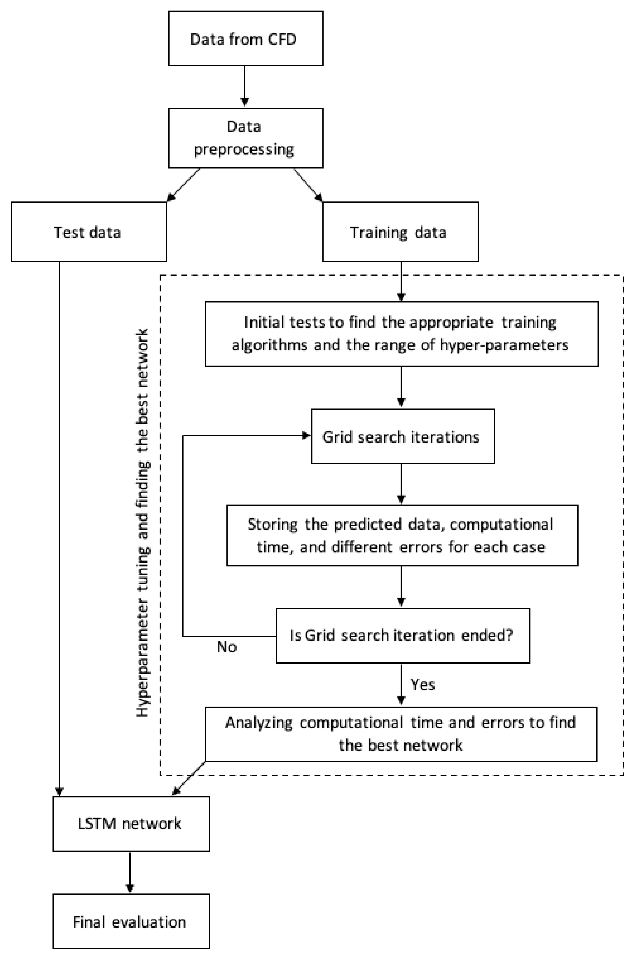
Given as a generalized algorithm, developing a model on the basis of an ANN should proceed as follows: (1) identification and collection of input/output data pairs (which in the present study are CFD-obtained gas parameters and soot volume fraction), (2) data preprocessing, (3) testing and optimization of the network architecture, (4) training the network, (5) testing the network, and (6) evaluation of the network predictions. Figure 5 illustrates the general model development procedure when using a deep learning approach. As in the previous study [17], data preprocessing was an essential step in obtaining satisfactory results. Recall that the core principle of training an artificial neural network is to update the network’s weights and biases such that the error between the network’s prediction and the actual outcome is minimized. Without some form of data preprocessing, differences in scale between the input and target data (potentially coupled with large variances within the data itself) may make the weights and biases hypersensitive to change. Updating the weights and biases in that kind of environment may lead to inaccuracies, low reproducibility, and inefficiency in the training process. Indeed, in the previous study [17], the greatest enhancement to the network’s predictive accuracy was the inclusion of data preprocessing. Prior to data preprocessing, the data was highly skewed (far from a normal distribution) and the network was predicting nonphysical results. The application of a log transformation gave a much more symmetric, bell-shaped distribution [17]. Similar results were obtained by Christo et al. [19] upon the application of a log transformation to their data set. In the current study, the unprepared data (both the input and target data sets) was processed by applying a log transformation and by standardizing the data (i.e., ensuring a mean of 0 and a standard deviation of 1).
The network architecture has a significant impact on training time and predictive accuracy. The time-dependent nature of this problem implied that LSTM layers should be the core of the network. Beyond this initial framework, it is important to realize that there is no definitive way to determine the ideal features of the neural network. This is due to the inherent complexity of a neural network. For example, consider the learning rate parameter. The learning rate of the network is the rate at which the weights and biases of the network are updated. While it is clear that the learning rate should not be too high (or else there may be instability in the training process), the optimal value is not immediately clear for a given problem.
Overfitting, one of the most significant issues in the training and application of ANNs, is a common example of a phenomenon that the network architecture impacts in a vague manner. Overfitting is a network behaviour that occurs when the predictive accuracy is higher for the training data than for the test data. The amount of overfitting is regarded as a measure of the general applicability of the network (i.e., the range of problems the network can successfully handle) and is a result of the network being excessively tuned to noise or specific features in the training data. The problem of excessive training can occur when there are many more trainable parameters (weights and biases) than data points. Consequently, a neural network with more layers or nodes is not guaranteed to give an increase in predictive accuracy. It is for this reason that structural parameters such as the number of hidden layers and number of nodes per layer become subject to experimentation.
The dropout process [39] is a regularization technique that is used to help reduce overfitting [32]. Dropout refers to the removal of certain nodes during the training process. Essentially, some nodes in a layer (chosen randomly) are dropped out and the network is trained without them for that iteration [32]. When the network is used after training, neurons are not dropped out. Rather, their output is scaled by 1 p , where p is the probability of being dropped out during training [
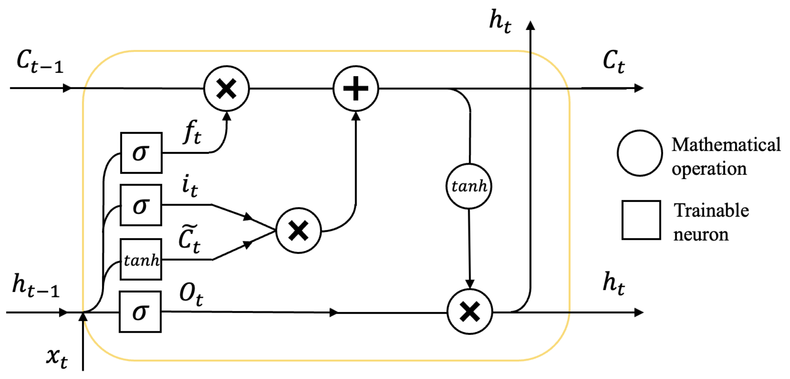
39]. Dropout may be thought of as an averaging process, where the final network has a predictive capability averaged over all the different networks from the training process (the networks with different nodes dropped out). Dropout aims to prevent the network from overemphasizing the importance of any specific piece of data in the training data set, hopefully broadening its range of use. In the current network, dropout is only applied between nodes transferring information in the same time step t [32], i.e., it is used in the vertical direction only (referring to Figure 2). The percentage of nodes to be dropped out and the number of layers to apply dropout on are more characteristics that must be tested.
In the present study, a grid search was performed to explore the parameter space and select the network with the best performance. The network’s accuracy and its computational time (time taken to train the network) are the major considerations in assessing network performance, with accuracy being the more dominant consideration. Readers are referred to the previous work [17] for more detail on the selection of the network parameters. The accuracy of the network was evaluated using 3 metrics: the relative error in the peak f v prediction, the relative error in the volume integral of f v across the whole domain, and the root mean squared error (RMSE), where all errors are relative to the CFD predictions. The error in peak f v measures the LSTM’s ability to predict the flame’s maximum soot concentration. The RMSE and error in the f v volume integral approximately quantifies the LSTM’s ability to predict the shape and distribution of the whole f v field. The errors for peak f v , the volume integral, and the RMSE are defined below in Equations (13,14,15), respectively. Note that in the discussion on the performance of the LSTM, Equations (13,14) are expressed in percentages.
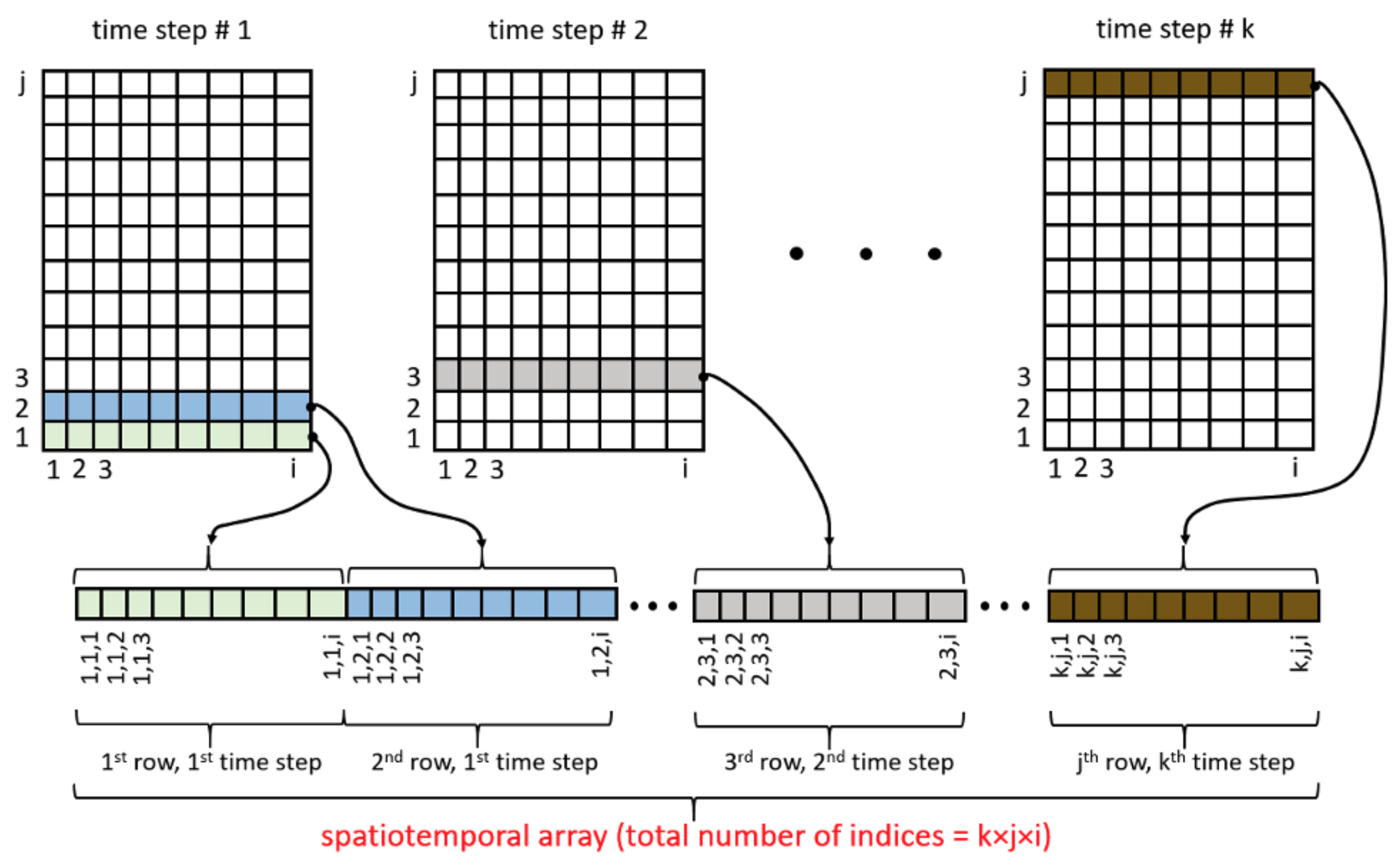
e p e a k = | f v m a x C F D f v m a x L S T M | f v m a x C F D
e i n t = | V 2 π r f v ( r , z ) d r d z C F D V 2 π r f v ( r , z ) d r d z L S T M | V 2 π r f v ( r , z ) d r d z C F D
R M S E = i = 1 n ( f v i C F D f v i L S T M ) 2 n
where r and z are the radial and axial coordinates in the 2D axisymmetric domain, respectively, i represents the index in the spatiotemporal array, and n is the total number of points in the spatiotemporal array.
The full list of hyperparameters and their tested values are shown in 
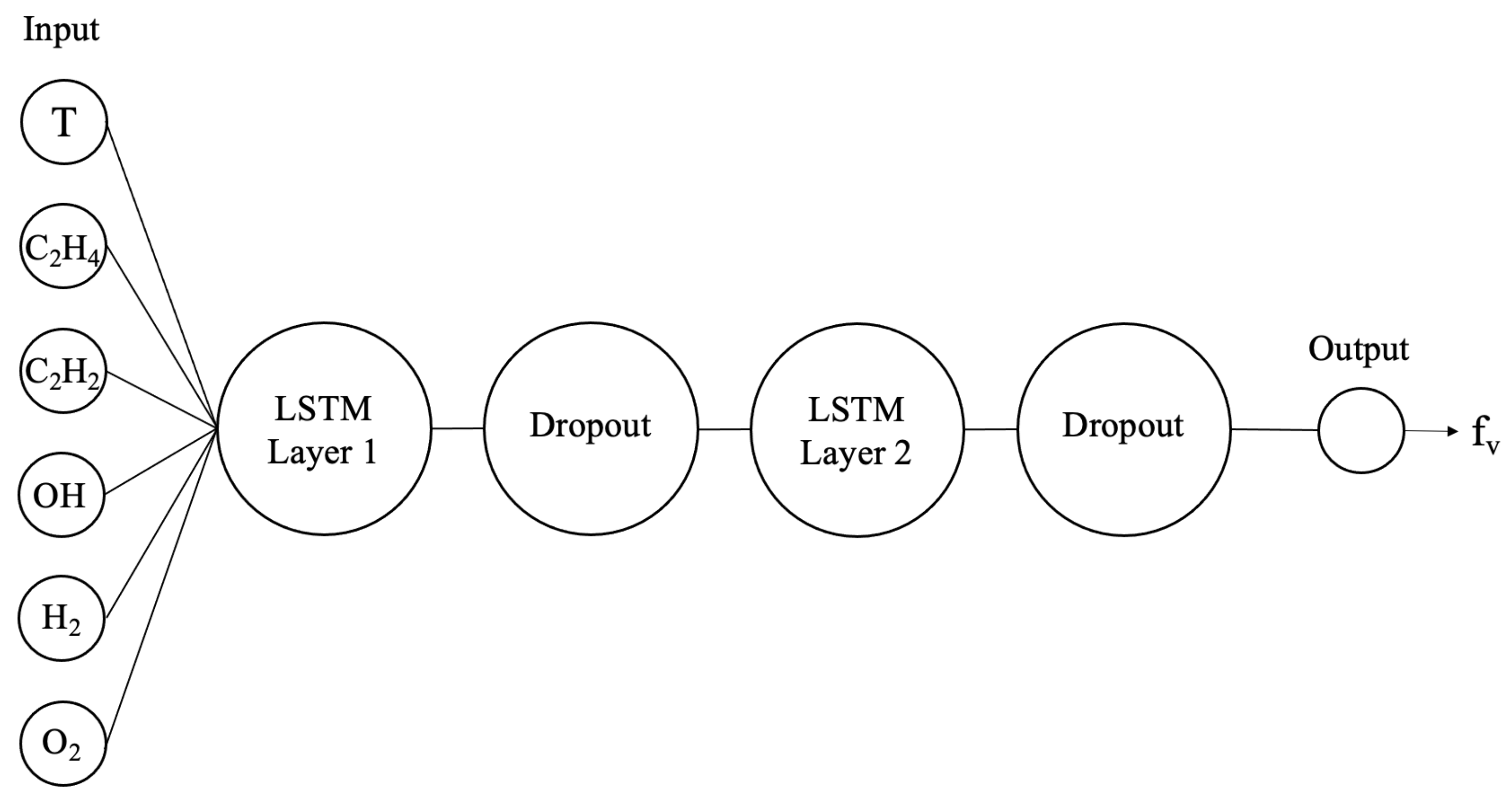
Table 1, where the parameters of the selected network are shown in bold. The selected network exhibited the best balance between accuracy and computational time, taking about 1 h to train on an NVIDIA GeForce GTX 1660 desktop graphics processing unit (GPU) and displaying good accuracy (to be discussed in detail below). A visualization of the final network is shown in Figure 6. Note that in Table 1, a dropout layer is not actually a layer of nodes. Rather, it signals that dropout has been applied to the previous layer of nodes. After the LSTM layers, there is a fully connected layer containing one node. This was the output node that returned the soot volume fraction and therefore was not changed throughout the grid search. For further information regarding the training options for a neural network, the reader is referred to the Mathworks documentation [40].
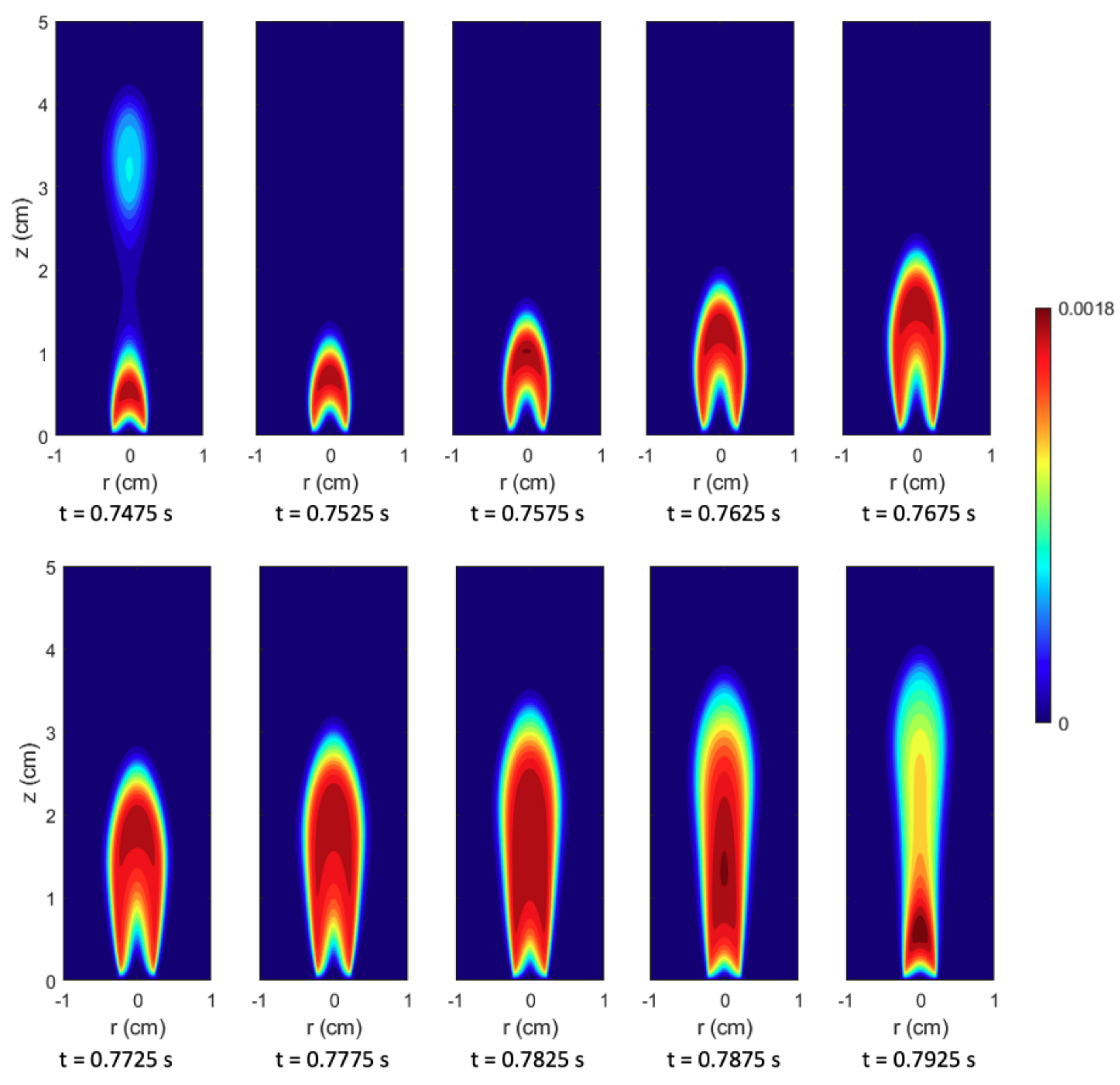
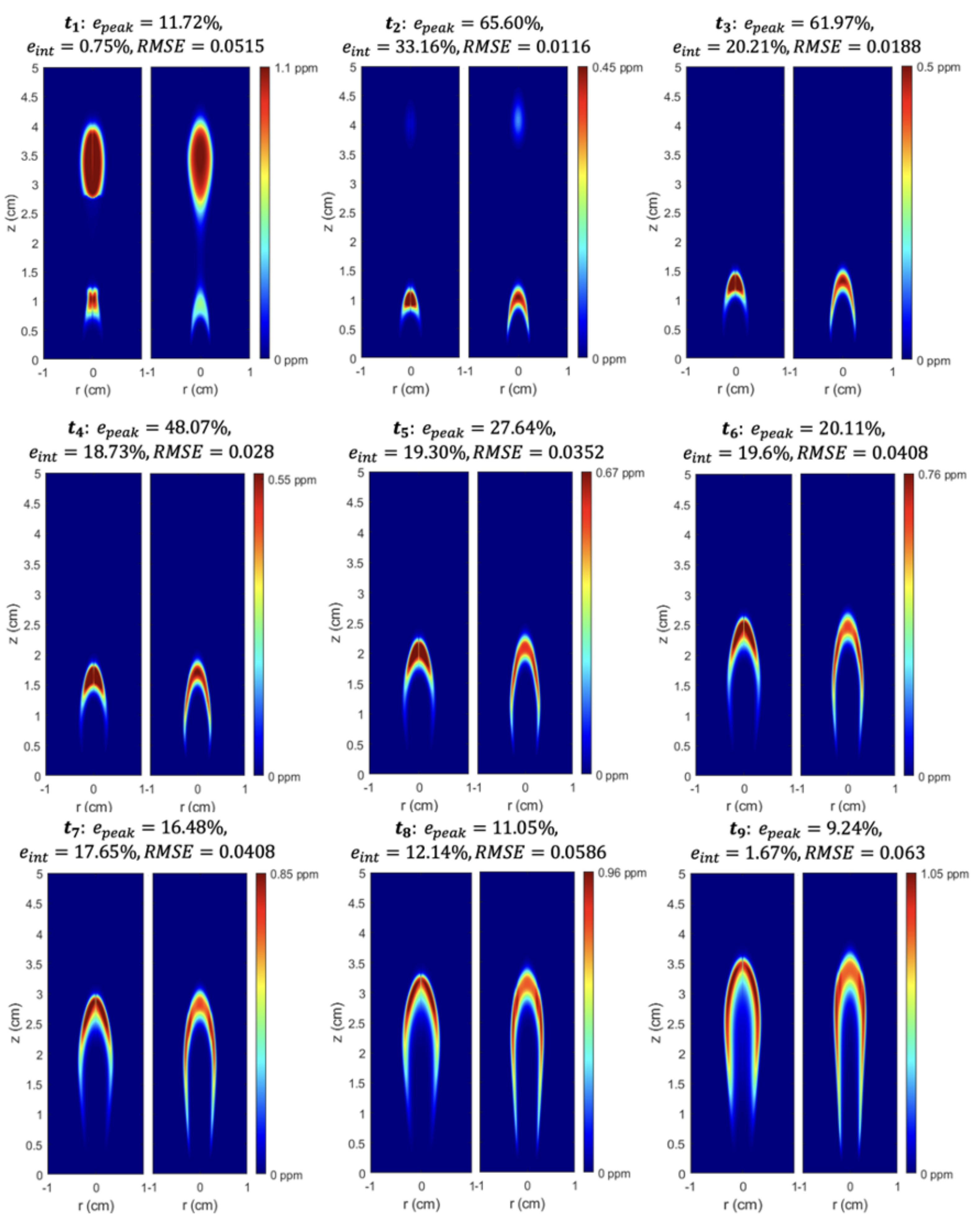
Figure 7 shows the predictions of the selected network compared to the CFD predictions. The images show the soot volume fraction at the 9 time steps in the training data set, where the left side is the prediction from the neural network and the right side is the CFD simulation. The network’s predictions on the training data match very well with the corresponding CFD prediction; the general shape and magnitude of the soot volume fraction contour is very similar between the CFD and the LSTM. The largest errors in e p e a k and e i n t (defined above in Equations (13) and (14)) occur in the earlier time steps, with accuracy steadily increasing from e p e a k = 65.60 % , e i n t = 33.16 % at t 2 to e p e a k = 9.24 % , e i n t = 1.67 % at t 9 . Note that the color bar on the right hand side of each pair of images corresponds to the CFD prediction. For example, at t 2 , the peak f v prediction from CFD was 0.45 and the peak prediction from the neural network was 65.60% higher than that (0.75 ppm). Table S1 in the Supplementary Materials shows the values of f v m a x , e i n t , and R M S E for CFD and the LSTM for each time step (rather than expressing them in a relative error percentage). The approximately fivefold decrease in e p e a k between t 2 4 and t 7 9 may be because the overall shape of the f v contour changes less rapidly at larger time steps, i.e., the change in f v shape from t 2 to t 5 is more pronounced than from t 5 to t 9 . Effectively, this may mean that the weights and biases are more tuned to predict an f v field that is similar to t 9 than one that is similar to t 2 (since there are more shapes in the training data that are similar to t 9 than to t 2 ). This may be resolved by including more data in the training data set that resembles the shape of the f v contour at t 2 .
Overall, the shape of the soot volume fraction contours predicted by the LSTM are very similar to the CFD contours. Early on ( t 1 to t 5 ), the neural network does not predict enough soot in the “tails”; however, this issue seemed to decrease as time increased (likely for the reasons stated in the previous paragraph). Even at t 1 , which is notably different than the rest of the time steps, the shape of the f v profile is fairly similar between the LSTM and CFD.
The average relative errors across all time steps in the training data were: e p e a k a v g = 30.21 % , e i n t a v g = 15.91 % , and R M S E a v g = 0.0393 . Despite the errors in peak f v for t 2 , t 3 and t 4 , the accuracy of the network is beyond satisfactory when one considers the massive reduction in computational time awarded by the neural network. As mentioned above, the selected neural network only took about 1 h to train on a desktop GPU, which is orders-of-magnitude less than the time it took to obtain a converged solution with CFD. The CFD calculations take on the order of 1 week to converge using approximately 400 CPUs. Furthermore, once the network was trained, it took seconds to run on the test data. This incredible speed-up, accompanied only by an average error of ∼30% in peak f v (relative to a high-fidelity CFD code) may be very valuable in an industry setting. In an industry use-case, high-fidelity CFD tools may not be practical and the designer may turn to semi-empirical soot models that are generally inaccurate yet expedient. Therefore, the availability of a soot estimating tool that can replicate a high-fidelty CFD model to within ∼30% in e p e a k and ∼15% in e i n t may not only facilitate the design cycle (through fast predictions), but provide an increase in accuracy relative to a semi-empirical model.
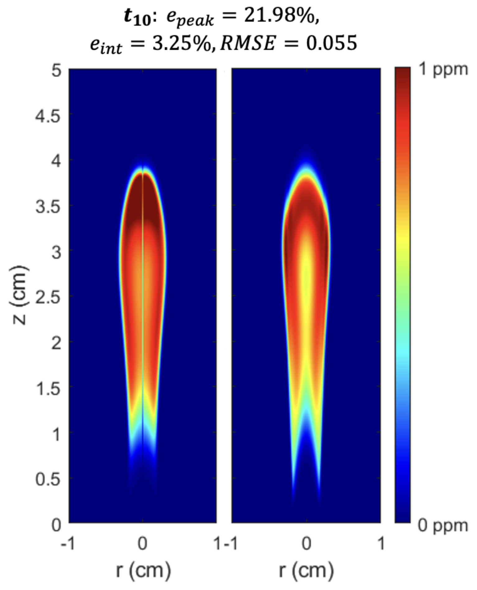
Figure 8 compares the prediction of the LSTM to CFD on the test data set (the 10 th time step). Recall that the test data was not used to update the weights and biases of the neural network and therefore represents an independent measure of the network’s accuracy and general applicability. The results on the test data were very reasonable: e p e a k = 21.98 % , e i n t = 3.25 % , and R M S E = 0.055 . The error with the LSTM predictions in the present study is comparable to the error in a recent study that used an LSTM to predict NO x emissions from a coal burner [32]; in both studies, the R M S E values were approximately 1–2 orders of magnitude lower than the magnitudes of the predicted quantities (i.e., soot and NO x ). In the results on the test data, there is perhaps some under-prediction of f v in the tails of the flame and some over-prediction of f v in the center and top; however, the overall shape and distribution of the f v field is quite similar between CFD and the LSTM.
The test results are encouraging because (1) e p e a k t e s t and e i n t t e s t were similar to e p e a k a v g and e i n t a v g from the training data set, indicating negligible overfitting and (2) the test results were fairly accurate despite the challenges associated with the f v contour at t 10 being qualitatively dissimilar to the f v contour from t 1 to t 9 . The fact that the network can still give reasonable accuracy (compared to CFD) for a f v contour that is dissimilar to the f v contours in the training data set indicates that it could potentially be applied to a wide range of problems. As in many problems that involve neural networks, the best way to increase the network’s general applicability is to broaden the training data set. Therefore, improvement to this network will involve an expansion of the training data set. Additional changes may be made to try to improve the accuracy of the prediction tool in future uses, including the use of a deeper network (more hidden layers) and an exploration of more advanced deep learning techniques (such as attention).
Given the novelty of the soot estimator and its potential application over a wide range of f v , it is appropriate to discuss different types of error. Equation (16) below was developed in [17] to analyze the absolute error for the soot estimator and will be applied here.
e = | 0 1 2 π r f v C F D ( r , z ) d r 0 1 2 π r f v L S T M ( r , z ) d r | 0 1 2 π r d r .
Equation (16) is only a function of z (axial height) because it is averaged in the radial direction. The averaging process in the radial direction reduces the error fluctuations significantly and makes the presentation and interpretation clearer. The error is averaged over r ∈ [0,1] because it covers the sooting region for all time steps.
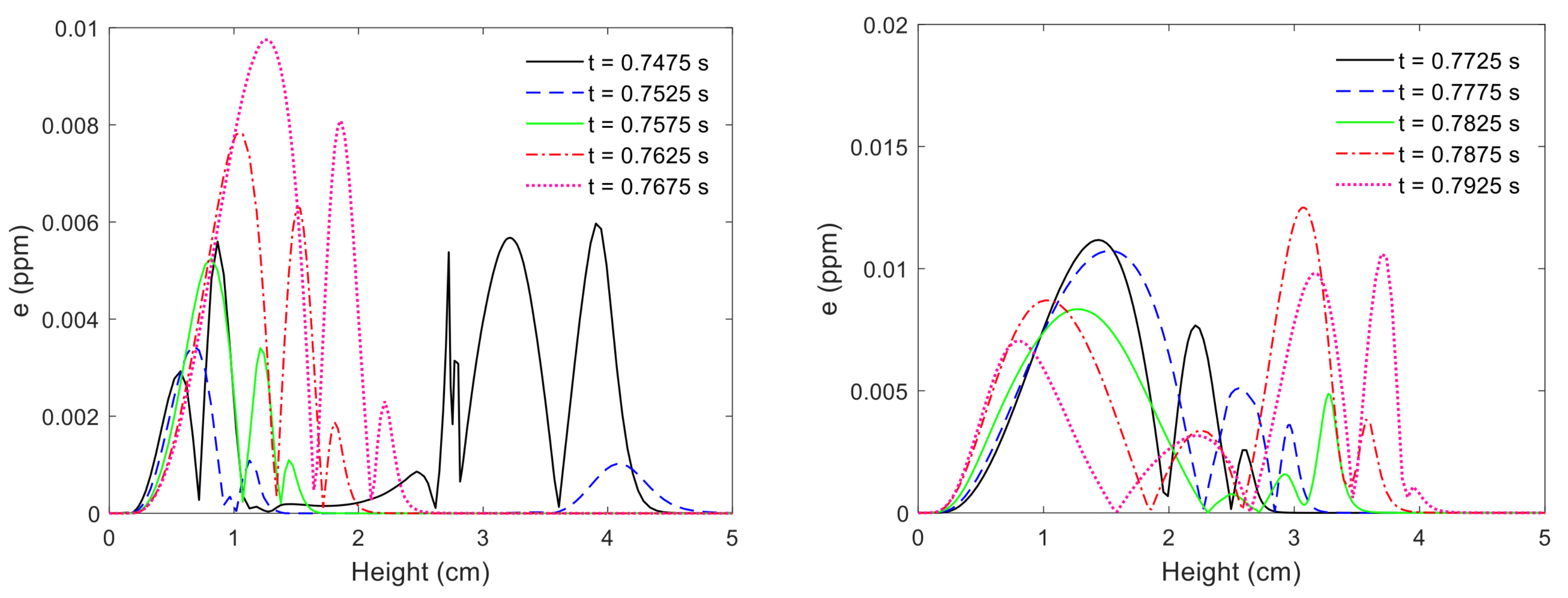
 Figure 9 shows e for all time steps in the training and test data (the test case is the largest time step). Interestingly, the largest values of e are for the time steps where e p e a k and e i n t are lowest, which indicates that the LSTM can give accurate predictions for all time steps if the predictions are averaged in the radial direction. Across all time steps, the maximum error is slightly over 0.012 ppm.
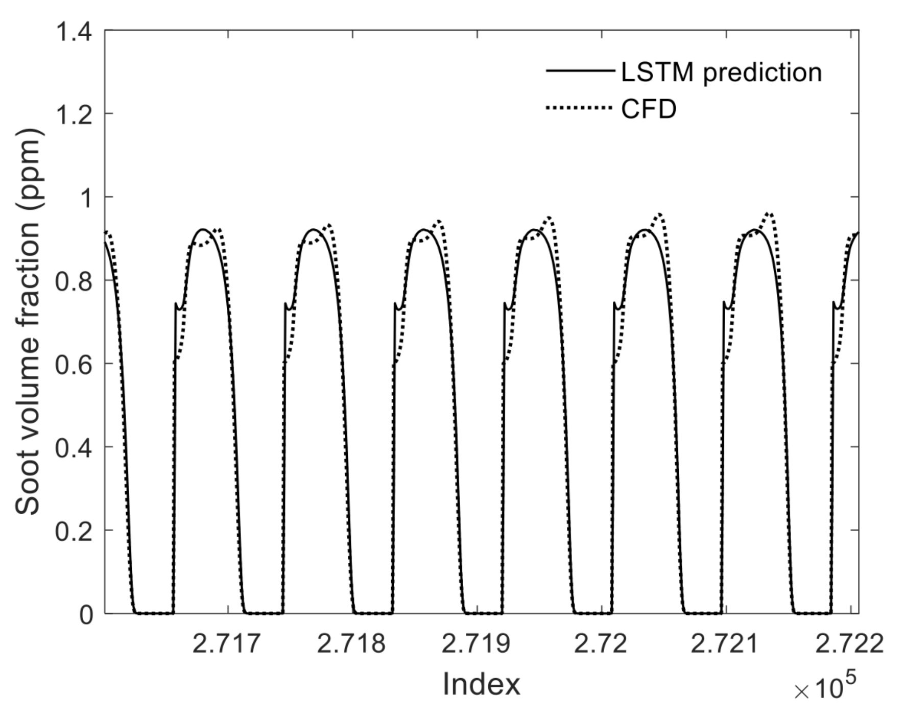
Figure 10 shows a graph of the LSTM and CFD predictions of soot volume fraction as a function of their index in the spatiotemporal array. Since the spatiotemporal arrays have tens of thousands of entries, the x-axis was limited to about 500 entries in order to improve readability. Figure 10 shows that the neural network can follow the CFD data across rapid changes in f v , which may bode well for its potential use in more complicated problems such as turbulent combustion. However, it remains to be seen whether this approach will thrive in a turbulent environment, where there may be many random or irregular changes in f v or any of the input parameters. The application of this LSTM to complex problems like transient, turbulent diffusion flames may be the subject of future works.

4. Conclusions and Recommendations

This study used an LSTM neural network to accurately estimate the soot volume fraction from a time dependent laminar sooting coflow diffusion flame, originally considered by Dworkin et al. in [33]. A high-fidelity CFD code was used to simulate this flame in Dworkin et al. [33] and the data from that simulation was used to train this neural network. The LSTM network received 6 input parameters from CFD (temperature and mass fractions of H 2 , C 2 H 4 , O 2 , O H , and C 2 H 2 ) and outputted soot volume fraction f v . The input data was collapsed into a spatiotemporal array and the network was trained on 9 consecutive time steps and tested on the 10th time step.
The input data was preprocessed by applying a log transformation and by standardization, which helped give a more normal distribution to the data, and subsequently, more accurate results to the network. The final LSTM neural network had 2 LSTM layers (each with 10% dropout), 100 LSTM hidden units per layer, and 35 epochs. The LSTM showed excellent estimation capability, closely matching the neural network in both shape and strength of the soot volume fraction contour for most time steps. The reduced computational time of the neural network compared to CFD is a major advantage; the trained LSTM only takes seconds to run on a modern desktop computer (after being trained for approximately 1 h), while a high-fidelity CFD model like CoFlame [2] may take weeks on a large supercomputer.
The successful implementation of this approach is a step forward in advancing the capabilities of the soot estimator idea. Although [32] has used LSTM neural networks to predict NO x emissions from a coal burner, this approach is, to the best of the authors’ knowledge, the first attempt to use an LSTM for soot prediction. Combined with the previous study [17], these works represent the first uses of neural networks to estimate soot concentration based on a detailed and high-fidelity CFD input. This detailed CFD input trained the network to recognize the foundational relationships between the gas phase properties and soot concentration. The reasonably accurate predictions on the training and test data bodes well for the use of the LSTM approach in more complex problems like transient, turbulent combustion. Overall, the success of the soot estimator tool in increasingly complex flames paves the way toward its adoption as the accurate, easy-to-use, and computationally inexpensive tool that the combustion industry acutely needs.

Supplementary Materials

The following are available online at https://www.mdpi.com/1996-1073/14/5/1394/s1, Figure S1: The contents of the spatiotemporal array for temperature. From top to bottom, the figure is zoomed in., Figure S2: The contents of the spatiotemporal array for soot volume fraction. From top to bottom, the figure is zoomed in., Table S1: The peak f v , volume integral, R M S E , and relative errors for LSTM and CFD at each time step.

Author Contributions

Conceptualization, M.J. and S.B.D.; methodology, M.J. and L.D.L.; software, M.J.; formal analysis, L.D.L.; writing—original draft preparation, L.D.L. and M.J.; writing—review and editing, L.D.L., M.J. and S.B.D.; supervision, S.B.D. All authors have read and agreed to the published version of the manuscript.

Funding

This research was funded by the Canadian Research Chairs Program, the Natural Sciences and Engineering Research Council of Canada (NSERC, grants. RGPIN-2019-04628 and RGPAS-2019-00123), and the Mitacs Research Training Award program.

Institutional Review Board Statement

Not applicable.

Informed Consent Statement

Not applicable.

Data Availability Statement

Not applicable.

Conflicts of Interest

The authors declare no conflict of interest.

References

  1. Shindell, D.; Kuylenstierna, J.C.; Vignati, E.; van Dingenen, R.; Amann, M.; Klimont, Z.; Anenberg, S.C.; Muller, N.; Janssens-Maenhout, G.; Raes, F.; et al. Simultaneously mitigating near-term climate change and improving human health and food security. Science 2012, 335, 183–189. [Google Scholar] [CrossRef] [PubMed] [Green Version]
  2. Eaves, N.A.; Zhang, Q.; Liu, F.; Guo, H.; Dworkin, S.B.; Thomson, M.J. CoFlame: A refined and validated numerical algorithm for modeling sooting laminar coflow diffusion flames. Comput. Phys. Commun. 2016, 207, 464–477. [Google Scholar] [CrossRef]
  3. Eaves, N.; Dworkin, S.; Thomson, M. The importance of reversibility in modeling soot nucleation and condensation processes. Proc. Combust. Inst. 2015, 35, 1787–1794. [Google Scholar] [CrossRef]
  4. Veshkini, A.; Eaves, N.A.; Dworkin, S.B.; Thomson, M.J. Application of PAH-condensation reversibility in modeling soot growth in laminar premixed and nonpremixed flames. Combust. Flame 2016, 167, 335–352. [Google Scholar] [CrossRef]
  5. Aubagnac-Karkar, D.; El Bakali, A.; Desgroux, P. Soot particles inception and PAH condensation modelling applied in a soot model utilizing a sectional method. Combust. Flame 2018, 189, 190–206. [Google Scholar] [CrossRef]
  6. Kholghy, M.R.; Veshkini, A.; Thomson, M.J. The core–shell internal nanostructure of soot–A criterion to model soot maturity. Carbon 2016, 100, 508–536. [Google Scholar] [CrossRef]
  7. D’Anna, A.; Sirignano, M.; Kent, J. A model of particle nucleation in premixed ethylene flames. Combust. Flame 2010, 157, 2106–2115. [Google Scholar] [CrossRef]
  8. Kholghy, M.R.; Eaves, N.A.; Veshkini, A.; Thomson, M.J. The role of reactive PAH dimerization in reducing soot nucleation reversibility. Proc. Combust. Inst. 2019, 37, 1003–1011. [Google Scholar] [CrossRef]
  9. Frenklach, M.; Mebel, A.M. On the mechanism of soot nucleation. Phys. Chem. Chem. Phys. 2020, 22, 5314–5331. [Google Scholar] [CrossRef]
  10. Mueller, M.E.; Pitsch, H. LES model for sooting turbulent nonpremixed flames. Combust. Flame 2012, 159, 2166–2180. [Google Scholar] [CrossRef]
  11. Mueller, M.E.; Pitsch, H. Large eddy simulation of soot evolution in an aircraft combustor. Phys. Fluids 2013, 25, 110812. [Google Scholar] [CrossRef] [Green Version]
  12. Tolpadi, A.K.; Danis, A.M.; Mongia, H.C.; Lindstedt, R.P. Soot Modeling in Gas Turbine Combustors. In Proceedings of the ASME Turbo Expo, Orlando, FL, USA, 2–5 June 1997. [Google Scholar]
  13. Brocklehurst, H.T.; Priddin, C.H.; Moss, J.B. Soot predictions within an aero gas turbine combustion chamber. In Proceedings of the ASME Turbo Expo, Orlando, FL, USA, 2–5 June 1997. [Google Scholar]
  14. Bozorgzadeh, S. Development of a Soot Concentration Estimator for Industrial Combustion Applications. Master’s Thesis, Ryerson University, Toronto, ON, Canada, 2014. [Google Scholar]
  15. Alexander, R.; Bozorgzadeh, S.; Khosousi, A.; Dworkin, S.B. Development and testing of a soot particle concentration estimator using Lagrangian post-processing. Eng. Appl. Comput. Fluid Mech. 2018, 12, 236–249. [Google Scholar] [CrossRef]
  16. Zimmer, L.; Kostic, S.; Dworkin, S. A novel soot concentration field estimator applied to sooting ethylene/air laminar flames. Eng. Appl. Comput. Fluid Mech. 2019, 13, 470–481. [Google Scholar] [CrossRef] [Green Version]
  17. Jadidi, M.; Kostic, S.; Zimmer, L.; Dworkin, S.B. An artificial neural network for the low-cost prediction of soot emissions. Energies 2020, 13, 4787. [Google Scholar] [CrossRef]
  18. Christo, F.; Masri, A.; Nebot, E.; Turányi, T. Utilising artificial neural network and repro-modelling in turbulent combustion. Proceedings of ICNN’95—International Conference on Neural Networks, Perth, Australia, 27 November–1 December 1995; Volume 2, pp. 911–916. [Google Scholar]
  19. Christo, F.; Masri, A.; Nebot, E.; Pope, S. An integrated PDF/neural network approach for simulating turbulent reacting systems. Symp. Int. Combust. 1996, 26, 43–48. [Google Scholar] [CrossRef]
  20. Ranade, R.; Alqahtani, S.; Farooq, A.; Echekki, T. An ANN based hybrid chemistry framework for complex fuels. Fuel 2019, 241, 625–636. [Google Scholar] [CrossRef]
  21. Pulga, L.; Bianchi, G.; Falfari, S.; Forte, C. A machine learning methodology for improving the accuracy of laminar flame simulations with reduced chemical kinetics mechanisms. Combust. Flame 2020, 216, 72–81. [Google Scholar] [CrossRef]
  22. Ranade, R.; Echekki, T. A framework for data-based turbulent combustion closure: A posteriori validation. Combust. Flame 2019, 210, 279–291. [Google Scholar] [CrossRef] [Green Version]
  23. Laubscher, R. Utilization of basic multi-layer perceptron artificial neural networks to resolve turbulent fine structure chemical kinetics applied to a CFD model of a methane/air piloted jet flame. J. Therm. Eng. 2018, 4, 1828–1846. [Google Scholar] [CrossRef]
  24. Li, S.; Yang, B.; Qi, F. Accelerate global sensitivity analysis using artificial neural network algorithm: Case studies for combustion kinetic model. Combust. Flame 2016, 168, 53–64. [Google Scholar] [CrossRef]
  25. Aceves, S.M.; Flowers, D.L.; Chen, J.Y.; Babajimopoulos, A. Fast Prediction of HCCI Combustion with an Artificial Neural Network Linked to a Fluid Mechanics Code; Technical Report, SAE Technical Paper; SAE: Warrendale, PA, USA, 2006. [Google Scholar]
  26. Blasco, J.; Fueyo, N.; Dopazo, C.; Ballester, J. Modelling the temporal evolution of a reduced combustion chemical system with an artificial neural network. Combust. Flame 1998, 113, 38–52. [Google Scholar] [CrossRef]
  27. Blasco, J.A.; Fueyo, N.; Larroya, J.; Dopazo, C.; Chen, Y.J. A single-step time-integrator of a methane–air chemical system using artificial neural networks. Comput. Chem. Eng. 1999, 23, 1127–1133. [Google Scholar] [CrossRef]
  28. Talebi-Moghaddam, S.; Bauer, F.; Huber, F.; Will, S.; Daun, K. Inferring soot morphology through multi-angle light scattering using an artificial neural network. J. Quant. Spectrosc. Radiat. Transf. 2020, 251, 106957. [Google Scholar] [CrossRef]
  29. Taghavifar, H.; Taghavifar, H.; Mardani, A.; Mohebbi, A.; Khalilarya, S.; Jafarmadar, S. Appraisal of artificial neural networks to the emission analysis and prediction of CO2, soot, and NOx of n-heptane fueled engine. J. Clean. Prod. 2016, 112, 1729–1739. [Google Scholar] [CrossRef]
  30. Ghazikhani, M.; Mirzaii, I. Soot emission prediction of a waste-gated turbo-charged DI diesel engine using artificial neural network. Neural Comput. Appl. 2011, 20, 303–308. [Google Scholar] [CrossRef]
  31. Alcan, G.; Yilmaz, E.; Unel, M.; Aran, V.; Yilmaz, M.; Gurel, C.; Koprubasi, K. Estimating soot emission in diesel engines using gated recurrent unit networks. IFAC-PapersOnLine 2019, 52, 544–549. [Google Scholar] [CrossRef]
  32. Yang, G.; Wang, Y.; Li, X. Prediction of the NOx emissions from thermal power plant using long-short term memory neural network. Energy 2020, 192, 116597. [Google Scholar] [CrossRef]
  33. Dworkin, S.; Cooke, J.; Bennett, B.; Connelly, B.; Long, M.; Smooke, M.; Hall, R.; Colket, M. Distributed-memory parallel computation of a forced, time-dependent, sooting, ethylene/air coflow diffusion flame. Combust. Theory Model. 2009, 13, 795–822. [Google Scholar] [CrossRef]
  34. Dworkin, S.B.; Zhang, Q.; Thomson, M.J.; Slavinskaya, N.A.; Riedel, U. Application of an enhanced PAH growth model to soot formation in a laminar coflow ethylene/air diffusion flame. Combust. Flame 2011, 158, 1682–1695. [Google Scholar] [CrossRef] [Green Version]
  35. Mueller, M.; Blanquart, G.; Pitsch, H. Hybrid method of moments for modeling soot formation and growth. Combust. Flame 2009, 156, 1143–1155. [Google Scholar] [CrossRef]
  36. LeCun, Y.; Bengio, Y.; Hinton, G. Deep learning. Nature 2015, 521, 436–444. [Google Scholar] [CrossRef] [PubMed]
  37. Hochreiter, S.; Schmidhuber, J. Long short-term memory. Neural Comput. 1997, 9, 1735–1780. [Google Scholar] [CrossRef] [PubMed]
  38. Yu, Y.; Si, X.; Hu, C.; Zhang, J. A review of recurrent neural networks: LSTM cells and network architectures. Neural Comput. 2019, 31, 1235–1270. [Google Scholar] [CrossRef] [PubMed]
  39. Srivastava, N.; Hinton, G.; Krizhevsky, A.; Sutskever, I.; Salakhutdinov, R. Dropout: A simple way to prevent neural networks from overfitting. J. Mach. Learn. Res. 2014, 15, 1929–1958. [Google Scholar]
  40. The Mathworks Inc. TrainingOptions. Available online: https://www.mathworks.com/help/deeplearning/ref/trainingoptions.html (accessed on 12 January 2021).
Figure 1. An illustration of an RNN network.
Energies 14 01394 g001
Figure 2. A schematic of the inner workings of an LSTM memory cell.
Energies 14 01394 g002
Figure 3. An example of part of the input data: H2 mass fraction at 10 time steps. The first 9 time steps is the training data while the last time step is the test data.
Energies 14 01394 g003
Figure 4. The concatenation process to convert the 3 dimensional input (time plus the axial and radial dimensions in space) into a spatiotemporal array. Every input variable, as well as the output variable of soot volume fraction, has its own spatiotemporal array.
Energies 14 01394 g004
Figure 5. A generalized algorithm for the development of an ANN-based model.
Energies 14 01394 g005
Figure 6. The architecture of the selected neural network. Note that the dropout bubbles are not their own layers of nodes, but they signal that dropout has been applied on the previous layer of nodes.
Energies 14 01394 g006
Figure 7. Soot volume fraction f v (ppm) compared at different time steps between CFD and the neural network (training data only). Left: LSTM neural network, right: CFD.
Energies 14 01394 g007
Figure 8. Soot volume fraction f v (ppm) compared between CFD and the neural network for the test data (the 10 th time step). Left: LSTM neural network, right: CFD.
Energies 14 01394 g008
Figure 9. Absolute error for all time steps. Left: time steps 1–5, right: time steps 6–10.
Energies 14 01394 g009
Figure 10. LSTM and CFD predictions of f v over a select range of the spatiotemporal index.
Energies 14 01394 g010
Table 1. Hyperparameters tested for the LSTM structure. Bold entries represent the selected hyperparameters.
No. of LSTM layers1, 2, 3
No. of dropout layers1, 2, 3
No. of hidden units/LSTM layer10, 20, 30, 50, 75, 100, 150, 200, 250, 300
No. of epochs20, 25, 30, 35, 50, 75, 100, 200, 300, 500, 1000
Gradient threshold0.1, 0.25, 0.5, 1, 1.5, 2, 5
Learning rate schedulePiecewise
Initial learning rate0.001, 0.005, 0.01, 0.05, 0.1, 0.2, 0.5
Learning rate drop period10, 20, 50, 100
Learning rate drop factor0.0001, 0.0005, 0.001, 0.005, 0.01, 0.05, 0.1
Dropout (%)1, 5, 10, 50
Training algorithmAdam, Stochastic Gradient Descent
Publisher’s Note: MDPI stays neutral with regard to jurisdictional claims in published maps and institutional affiliations.

