Article

Learning to Calibrate Battery Models in Real-Time with Deep Reinforcement Learning

ETH Zürich, Rämistrasse 101, 8092 Zürich, Switzerland
*
Author to whom correspondence should be addressed.
Energies 2021, 14(5), 1361; https://doi.org/10.3390/en14051361
Submission received: 27 January 2021 / Revised: 16 February 2021 / Accepted: 22 February 2021 / Published: 2 March 2021

Abstract

:
Lithium-ion (Li-I) batteries have recently become pervasive and are used in many physical assets. For the effective management of the batteries, reliable predictions of the end-of-discharge (EOD) and end-of-life (EOL) are essential. Many detailed electrochemical models have been developed for the batteries. Their parameters are calibrated before they are taken into operation and are typically not re-calibrated during operation. However, the degradation of batteries increases the reality gap between the computational models and the physical systems and leads to inaccurate predictions of EOD/EOL. The current calibration approaches are either computationally expensive (model-based calibration) or require large amounts of ground truth data for degradation parameters (supervised data-driven calibration). This is often infeasible for many practical applications. In this paper, we introduce a reinforcement learning-based framework for reliably inferring calibration parameters of battery models in real time. Most importantly, the proposed methodology does not need any labeled data samples of observations and the ground truth parameters. The experimental results demonstrate that our framework is capable of inferring the model parameters in real time with better accuracy compared to approaches based on unscented Kalman filters. Furthermore, our results show better generalizability than supervised learning approaches even though our methodology does not rely on ground truth information during training.

1. Introduction

Recent advancements in lithium-ion (Li-I) battery technology have increased their usage in various applications ranging from electric vehicles to drones [1], smart grids [2], and space exploration [3]. Particularly for autonomous systems, it is essential to plan the missions reliably, which requires an accurate prediction of the end-of-discharge (EOD) time for the batteries. Several battery models have been introduced to model the discharge process of the batteries for accurate prediction of EOD [4,5,6]. However, most of these models suffer from an increasing uncertainty in their EOD predictions over time [7]. This is because the batteries degrade with aging and computational models suffer from a reality gap between the physical process and the simulated one. The relationship between battery age and degradation parameters is complex and requires sophisticated modeling techniques to estimate battery degradation parameters that are part of the EOD time prediction [8]. Estimating degradation parameters of the battery model is also known as “model calibration” [9]. Hence, we use these terms interchangeably in this manuscript.
Previous research studies on battery model calibration have mainly focused on understanding and modeling the electrochemical aging processes [8,10,11]. Such methods are known as prognostics and health management (PHM) models, which assume an underlying model for the aging process. However, the calibration problem can also be modeled as a parameter tracking and inference problem. The model parameters are then inferred from the empirical observations. Previous works have focused on traditional variants of Kalman filters, such as the extended Kalman filter (EKF) and unscented Kalman filter (UKF) [12,13], or Bayesian filters such as particle filters, [14] for tracking degradation parameters of the batteries. Parameter tracking approaches do not require an underlying degradation model. However, they suffer from a high computational burden and parameter divergence problems. Several data-driven methods based on empirical learning models have also been proposed for battery end-of-life (EOL) or state of health (SOH) prediction [12,15]. These supervised data-driven methods suffer from a strong dependence on labeled data, also requiring for each training sample the ground truth calibration parameters. However, measuring the ground truth values of the degradation parameters during operation is not practical in many scenarios. These shortcomings limit the applicability of the supervised data-driven approaches in real-world problems.
Reinforcement learning (RL) provides an alternative to parameter tracking approaches by formulating real-time calibration as a Markov decision process (MDP). Combined with powerful function approximators, such as deep neural networks, RL methods can work with complex large-state spaces. RL methods have been applied to various control problems in robotics [16,17,18], water systems management [19], computational biology [20], and AutoML [21]. RL methods have multiple advantages over traditional methods: (1) RL agents can learn to solve tasks without any knowledge of the underlying model. Such methods are known as model-free methods that directly learn by sampling interactions from the environment [22]. (2) The policies learned via RL are robust to model uncertainty [23]. (3) RL methods provide almost real-time performance since they only require evaluating the learned policies. These characteristics make reinforcement learning a compelling alternative to other data-driven methods for battery model calibration.
In this paper, we adopt a reinforcement learning framework [24] to solve the battery model calibration process, which can work in real time and does not require an underlying degradation model. Specifically, we define the battery model calibration problem as a tracking problem using MDP and solve it with the Lyapunov-based maximum entropy reinforcement learning algorithm [24]. We use the battery model from the NASA prognostic model library [25,26] to simulate the RL environment. It is important to emphasize that the applied simulation method models the physical process of the discharge but does not explicitly model the battery aging process, which is the main focus of this paper. To the best of our knowledge, the framework proposed here is the first method applying reinforcement learning to battery model calibration.
The remainder of this paper is structured as follows. In Section 2, we discuss related work. In Section 3, we present the battery discharge model and our reinforcement learning-based calibration framework. In Section 4, we present the datasets, model design, and comparison methods. We discuss our findings in Section 5.

2. Related Work

In this section, we provide a brief overview of three primary methods for battery model calibration: (1) methods based on Bayesian tracking principle; (2) model-based prognostics based on an explicit aging model; (3) direct estimation from observations.
Firstly, methods based on filtering approaches model the parameters of the battery as an internal state and try to track these parameters by external observations. Variants of Kalman filters, such as the unscented Kalman filter (UKF) [13] and extended Kalman filter (EKF) [12] have been used to calibrate battery models. Particle filtering (PF) approaches are similar to UKF. PF-based approaches try to approximate the probability density function of the battery parameters using particles [14]. However, particle filters suffer from particle degeneracy, which results in large estimation errors. The authors of [27] proposed inheritance-based particle filtering to tackle this problem. Such tracking algorithms provide model-agnostic parameter estimations. However, these methods are computationally expensive at the application time and suffer from a drift in parameter tracking.
Secondly, model-based prognostic methods assume an underlying degradation model for the aging parameters as a function of its usage. The authors of [8] used system identification techniques to estimate the parameters of the degradation model. Furthermore, the authors of [10,11] used electrochemical process knowledge to model battery degradation. These techniques provide accurate estimates as long as the physical degradation process follows the assumed model.
Thirdly, in the direct estimation methods, observations are used to learn the mapping from the battery outputs to the degradation parameters. For example, the authors of [15] used support vector machines (SVM) to learn this mapping. In another study, structured neural networks (SNN) were used to exploit knowledge of the degradation process [12]. Such approaches show promising results in certain scenarios where it is possible to obtain a representative set of labeled samples comprising observations and degradation parameters covering all relevant operating conditions.
Reinforcement learning provides an alternative solution to these three types of approaches while overcoming some of their limitations. Especially, in the scenarios where labeled data are not available, RL can learn from the observations and infer the model parameters. Furthermore, RL is typically computationally very efficient in real-time applications compared to the model-based Kalman filter and its variants. Previous works have highlighted the importance of reinforcement learning in SOH estimation and battery scheduling operations. The authors of [28] used reinforcement learning to estimate the parameters of EKF, which in turn was used to estimate SOH for the batteries. Our method goes one step beyond this—we try to estimate the parameters directly from the observations. Hence, we remove the dependence on the model-based EKF approach. The authors of [29] also highlighted the effectiveness of reinforcement learning in designing an optimal control policy to reduce transmission losses.
With deep function approximators and sophisticated exploration techniques, RL methods have recently made some significant progress. In our work, we focus on model-free RL methods based on the actor–critic (AC) approach [22,30]. Model-free methods can learn the policy without knowing the underlying model. Actor–critic methods provide a framework for generalized policy iteration algorithms in which two networks (actor and critic) are updated continuously. Especially, maximum entropy-based RL formulation such as soft actor–critic (SAC) [31,32] algorithms have shown good performance in different applications [33,34]. Tian et al. [24] proposed a variant of the maximum entropy-based RL algorithms for the model calibration of turbofan engines. In that work, the authors proposed to use the Lyapunov-based critic (LAC) approach, which has been proven to provide guaranteed stable control [23]. We adapt the proposed approach to the battery calibration problem.

3. Materials and Methods

As discussed earlier, to solve calibration using reinforcement learning, we need to define the environment for our RL agent. We integrate the battery discharge model described below in OpenAI gym [35] to build the RL environment. We also discuss our RL framework and propose to use a Lyapunov actor–critic [23] algorithm for battery model calibration.

3.1. Battery Discharge Model

In this research, we apply the Li-I battery model from NASA the prognostic model library [25,26]. It captures significant electrochemical processes of the discharge. The effect of aging is included in the model by the corresponding degradation parameters. However, the degradation is not modeled explicitly. The model assumes that the degradation parameters are provided. Those are essential for an accurate estimation of the EOD time.
The battery state is modeled by seven parameters as described below. The state changes over time as a function of input load and degradation parameters. In the following, we just denote the state mathematically and refer the readers to the original paper for more details on the battery model [25].
x t = [ q s , p q b , p q b , n q s , n V o V η , p V η , n ] ,
In the first four parameters in Equation (1), q represents the amount of charge, subscript p (or n) represents positive (or negative) electrodes, respectively, and subscript s (or b) represents the surface (or bulk) volume of a particular electrode, respectively. For example, q s , p is the amount of surface charge in the positive electrode. V η , n and V η , p are the voltage drops due to surface over potential on negative and positive electrodes, respectively. V o is the total voltage drop.
There are two main degradation parameters: (a) Q m a x captures the decrease in available lithium ions, and (b) R o captures the increase in the internal resistance. These parameters are essential for the model dynamics that is defined as follows:
x t + 1 = f ( x t , u t , Q m a x , R o ) , y t + 1 = g ( x t + 1 , Q m a x , R o ) ,
where u t represents the input load at time t, and the model predicts the battery voltage y t = V . f and g are the functions for the system dynamics and output measurements, respectively.
Without any knowledge of the battery age, degradation parameters are initialized to the “perfect battery” condition values, which are Q m a x = 7600 C and R o = 0.117215 Ω [25]. Using these parameters, the model can estimate the initial state x 0 . As the battery ages, Q m a x decreases while R o increases. We learn to infer these parameters by solving the state-tracking problem using RL. In this research, we used the NASA prognostic battery model [25] as our reinforcement learning simulation environment. However, in cases where such a model is difficult to obtain, it can be replaced by surrogate models.

3.2. Markov Decision Process and Reinforcement Learning

In this paper, we focus on the battery state tracking task, which we propose to model as a Markov decision process (MDP). An MDP can be described as a tuple, < S , A , C , T , ρ >, where S is the set of states, A is the set of actions, C ( s , a , s ) [ 0 , ) is the cost function, T ( s , a , s ) = p ( s | s , a ) is the transition probability function, and ρ ( s ) is the initial probablity distribution over the states. The policy π θ ( a | s ) denotes the probability of selecting action a in state s , and it is parameterized by the parameters θ . The state of the MDP at time t is defined as s t S R n , where S denotes the state space. For the proposed tracking strategy, we define the state at time t as s t = [ x ^ t , x t + 1 , u t + 1 ] , where x ^ t is the battery’s internal state produced by the battery discharge model at time t, x t + 1 is the real (or simulated) battery state we want to achieve at time t+1, and u t + 1 is the input load condition at time t+1. The agent (calibrator) then controls the system’s degradation parameters as an action a t A R m (e.g., a t = Q m a x or R o or [ Q m a x , R o ] ) according to the policy π ( a t | s t ) . Based on the internal state x ^ t and predicted action a t , we simulate the next internal state x ^ t + 1 = f ( x ^ t , a t , u t + 1 ) , where f is the battery discharge dynamics described in Equation (2). Hence, the cost function c ( s t , a t ) = | | x ^ t + 1 x t + 1 | | denotes the quality of action a t to go from x ^ t to x t + 1 at load condition u t + 1 . During the entire learning process, the agent never observes true degradation parameters. The agent learns to control the degradation parameters by minimizing the cost formulated using the observations. After one complete transition, the next state of the MDP is s t + 1 = [ x ^ t + 1 , x t + 2 , u t + 2 ] . This complete process is demonstrated in part (1) of Figure 1. Once the policy network is trained, it can work as a calibrator, where it observes the state from the real system and outputs its parameters for the computer model (part (2) of Figure 1).

3.3. Lyapunov-Based Actor–Critic

Since we target the state tracking task, we adopted the Lyapunov-based actor–critic (LAC) approach as proposed in [23]. LAC was designed to improve the stability of the reference trajectory tracking problems by incorporating a Lyapunov energy decreasing constraint as defined in Equation (3) in the policy objective:
E s τ ( E s T π L ( s ) L ( s ) ) α 3 E s τ C π ( s ) ,
where L ( . ) is the Lyapunov value function, α 3 is a positive constant, and the other notations are the same as described before.
Hence, our policy network is trained to minimize the energy decreasing Lyapunov objective J c ( π ) E τ π t = 0 N L ( s t + 1 ) L ( s t ) + α 3 C π ( s t ) , where N is the number of steps for a single state tracking iteration.
Based on the actor–critic framework, LAC uses the Lyapunov function L c ϕ as a critic in the policy gradient formulation. Similar to value function learning, the Lyapunov function is also parameterized by a neural network ϕ . This network is trained to minimize the following objective:
J ( L c ) = E ( s , a ) D 1 2 ( L c ϕ ( s , a ) L c t a r g e t ( s , a ) ) 2
where L t a r g e t is the approximation target related to the chosen Lyapunov candidate and D is the set of collected transition pairs. The approximation target is given by:
L c t a r g e t = c + max a γ L c ϕ ( s , a )
LAC is based on the maximum entropy-based actor–critic framework [31], which can enhance the exploration of the policy and has been shown to substantially improve the robustness of the learned policy. Hence, our actor network ensures stable and robust control of the degradation parameters. The full objective for the policy network is defined as follows:
J ( π ) = E D [ β [ log ( π θ ( f θ ( ϵ , s ) | s ) ) ] + λ ( L c ( ( s , f θ ( ϵ , s ) ) L c ( s , a ) + α 3 c ) ]
where π θ is the policy parameterized by a neural network f θ and ϵ is an input vector consisting of Gaussian noise. D { ( s , a , s , c ) } is the replay buffer for storage of the MDP tuples. In the above objective, β and γ are positive Lagrange multipliers that control the relative importance of policy entropy versus the stability guarantee, and α 3 is a constant for a Lyapunov energy decreasing objective. Similarly to the approach applied in the [31], the entropy of the policy is expected to remain above the target entropy H t . The values of β and λ are learned through the gradient method, thereby maximizing the following objectives:
J ( β ) = β E ( s , a ) D [ log ( π θ ( a | s ) ) + H t ]
J ( λ ) = λ ( L c ( ( s , f θ ( ϵ , s ) ) L c ( s , a ) + α 3 c ) .

4. Experiment Datasets and Models

In this section, we discuss simulated data generation using battery discharge model described in Section 3.1. We also discuss the Unscented Kalman Filter (UKF) and the direct mapping methods to compare them with our approach.

4.1. Dataset Generation

As mentioned above, we used the battery model from the NASA prognostic model library [26] to generate simulated data for the training process. As discussed earlier, we have two degradation parameters to calibrate in a battery model. We propose two different experiments for the tracking: (1) Only varying a single parameter at a time. Hence, while varying Q m a x , R o was kept constant (at 0.117215 Ω ) and while varying R o , we kept Q m a x constant (at 7600 C, C = Coulomb). (2) Varying both parameters simultaneously. For the first experiment, we generated trajectories by varying Q m a x between 4000 and 7000 C with 501 grid values of constant length in between and keeping R o constant at 0.117215 Ω . We also generated discharge trajectories by varying R o between 0.1 and 0.2 Ω with 501 grid values while keeping Q m a x constant at 7600 C. For the second experiment, we varied both the parameters, i.e., Q m a x between 4000 and 7000 C and R o between 0.1 and 0.2 Ω simultaneously. Following the approach of [8], we kept degradation parameters constant for a given discharge cycle. Furthermore, we generated each discharge trajectory for 11 different input load (u) conditions between 8 and 16 W. For each trajectory, the battery state defined in Equation (1) was initialized based on the degradation parameter values for that particular trajectory; namely, the voltage drops ( V o , V η , p , V η , n ) were initialized with 0 and the charges ( q s , p , q b , p , q b , n , q s , n ) were initialized proportional to Q m a x following [25]. Hence, the trajectories with different degradation parameter values went through different discharge cycles. Each trajectory was simulated until the output voltage reached the EOD threshold (3 V). The simulated datasets’ generation is explained in more detail in Appendix A.

4.2. Hyperparameters of the RL Framework

We adopted the same neural network architecture as applied in [24]. We used a fully connected neural network as a function approximator for our actor, f θ , and Lyapunov critic, L c . Both networks had three fully connected layers with 256 neurons each and LeakyReLU [36] activation functions. For the policy network, we predicted two values, namely the mean and the standard deviation for each action. After this step, we used the squashed Gaussian policy [31] to sample from the distribution. To ensure that the Lyapunov values are positive, we used the sum-of-squares of the final layer activations of the Lyapunov network as Lyapunov values. We used α 3 = 1 for the energy decreasing condition described in Equation (3). The parameters β and λ were also updated using the loss defined in Equations (7) and (8). We used an Adam optimizer with the learning rate 5 × 10⁻⁴.

4.3. Compared Methods

We compared the proposed model calibration methodology to the two alternative methods that are comparable to the proposed framework: on the one hand to methods based on Bayesian tracking principles, in particular to the unscented Kalman filter, and on the other hand to a supervised data-driven direct estimation.

4.3.1. Unscented Kalman Filter (UKF)

We compared our RL approach to the traditional unscented Kalman filter (UKF). Here, we used the UKF approach proposed in [37]. A UKF models the degradation parameters as a hidden state and the battery model state as an observation. In particular, the hidden state for the UKF was z { Q m a x , R o } ( z R 2 ) and the observation was the battery state defined in Equation (1) ( x R 7 ). The UKF starts with a distribution over the initial state and this state distribution is continuously modified through unscented transformations to generate the distribution over the hidden state at each time step. Since we kept the degradation parameters constant throughout one discharge cycle, the UKF state update equation and observation equation were defined as follows:
z ^ t + 1 = z ^ t x ^ t + 1 = f ( x ^ t , u t + 1 , x ^ t + 1 ) ,
where f is the observation function for the UKF, which was obtained from the battery model introduced in [25], and u is the input load. The initial state z ^ 0 was initialized as a multi-variate standard normal distribution. At the start of each new trajectory, UKF restarts its tracking (i.e., the state is reinitialized with z ^ 0 ). Without a restart, the UKF might diverge since there is no connection between two different discharge cycles. Furthermore, the UKF parameters were fine-tuned for the battery discharge datasets described in Section 4.1.

4.3.2. Direct Mapping

We also considered a fully connected neural network to learn a direct mapping from state s t to the degradation parameters (corresponding to a t in the RL setting). It is important to emphasize that direct mapping is a much simpler problem compared to inferring the calibration parameters via the tracking problem without any access to the ground-truth calibration parameters. In direct mapping, the algorithm learns from the labeled pairs of “states” and “degradation parameters”. This set of representative labeled samples might not be easy to obtain in real-world scenarios. For each state of the asset, the underlying degradation parameters need to be measured manually, which is considerably time-consuming. Furthermore, the training datasets are required to be representative and cover all the different combinations in all relevant operating conditions to enable a reliable machine learning (ML) model. Hence, the results obtained with this supervised learning setup can be considered as an upper bound for the proposed RL framework performance for the cases where the training and the testing datasets come from the same distribution.
For the direct mapping experiment, we used the same architecture as the policy network described in Section 4.2, with the difference being that only one output per action was learned since the standard deviation was not required. We used the same optimizer and hyperparameters as described in Section 4.2.

5. Results

We divided the generated discharge trajectories into 70% training and 30% testing datasets. The input load conditions represented in the training and testing datasets did not overlap. Hence, the results presented here are suitable to assess the generalization capability of our method. We trained our RL model for one million steps, which resulted in reward convergence. For direct mapping, we trained the model until the L2-loss between predicted parameters and ground truth values converged.
We compared the inference accuracy of our RL-based approach to the UKF method and the direct mapping approach. Furthermore, as described in Section 4.1, we conducted single- and multi-parameter evaluation experiments. We report the normalized root mean squared error (RMSE) between the ground truth parameters and predicted parameters in Table 1. Parameters were scaled between 0 and 1 for the RMSE calculation. Furthermore, the numbers represent % RMSE (i.e., normalized RMSE x 100)
The proposed RL-LAC reduced the % RMSE by more than 50% compared to the traditional UKF tracking approach. Even in multi-parameter tracking, we can see that RL-LAC consistently outperformed UKF. As discussed earlier, the direct mapping method can work better than RL when the test data come from the same distribution as the training data. In our case, the testing trajectories had different load conditions than the training trajectories. Hence, for a single parameter R o tracking, we observed the training error of 0.3% while the test error increased to 10.2%. This shows the limitation of the direct mapping approach and highlights the fact that it can suffer from a generalization gap if not trained on data that are representative of the application. The direct mapping method had a negligible error for parameter Q m a x in both the experiments, since Q m a x can be derived exactly from our state formulation. This has also been highlighted in the battery discharge model [25]. However, as discussed earlier, direct mapping requires ground truth degradation parameters, which are difficult to obtain in real-world applications.
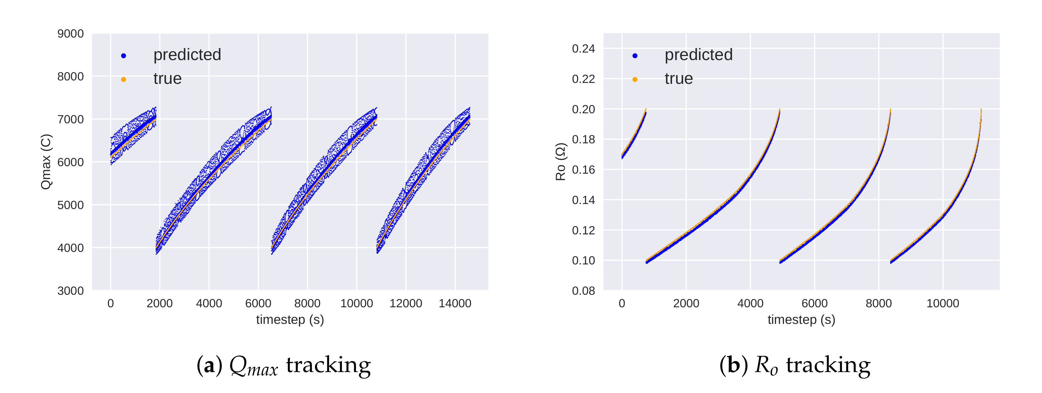
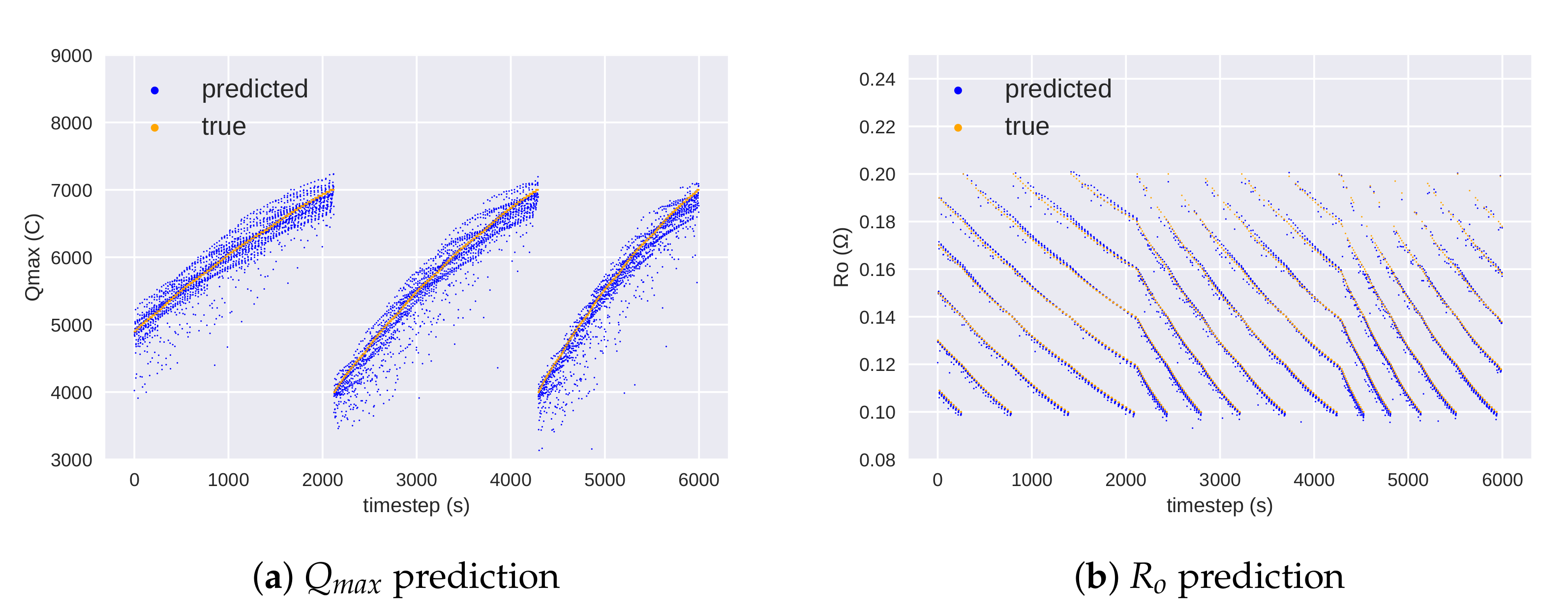
To further investigate the performance of the proposed framework, we show inference results of the degradation parameters for single parameter tracking experiments (in Figure 2), and for a multi-parameter tracking experiment (in Figure 3). In Figure 2, each trajectory represents a different load condition. It is important to point out here that our RL-based method works independently on each discharge cycle, and hence, the order of the parameters does not matter. Additionally, this implies that the calibration errors across discharge cycles are not self-correlated. For both experiments, even though there was some variance in the inference of the parameter Q m a x , we can see that most of the points were close to the true parameters, whereas in the case of R o , tracking accuracy was better than that of Q m a x . Interestingly, our tracking never diverged too much from the ground truth parameters, which shows the effectiveness of using the Lyapunov-based stability guarantee in our RL framework.
In Table 2, we present the inference times for all three methods. The time has been calculated by averaging five different runs of 2000 random transitions on a single-core CPU. As discussed earlier, model-based methods (such as UKF) require multiple battery model evaluations at each step, and hence they have the highest inference times. On the other hand, inference time for our RL method depends on the complexity of the policy network, and it was more than twice as fast as the applied UKF. Furthermore, with increasingly complex battery models, inference time for the UKF will increase proportionally, whereas for the RL, it will remain similar. Direct mapping methods were found to run much faster at deployment time than any other methods as expected.

5.1. Discussion

In summary, the performance of the RL method was consistently better than traditional tracking methods such as UKF, while being able to perform stable, real-time tracking of the parameters. In addition, the reinforcement learning agent can generalize on out-of-distribution load conditions and is able to accurately track parameters for the test load conditions, whereas the direct mapping method suffers from a lack of generalization. This competitive performance is achieved while purely learning from the interactions and without any access to the ground truth.

5.2. Limitations

Our RL-based method enables accurate calibration of the battery model. However, our method has only been tested on simulated data. Sim-to-real transfer of the RL agent is an active research topic [38], and our proposed algorithm needs to be further tested on the real degradation process data. Furthermore, along with the point estimate of the degradation parameters, the confidence interval of the predictions can help in the maintenance scheduling of the batteries. Incorporating uncertainty into RL agents’ decisions is also an actively studied topic [39], and the research in this field can be incorporated with our method to enhance the reliability of the proposed algorithm.

6. Conclusions

In this paper, we presented a new approach for battery model calibration formulated as a tracking problem. We solved this tracking problem using a Lyapunov-based maximum entropy reinforcement learning framework and showed that the inference of this model provides accurate estimates of the model parameters. The performance of the RL framework presents an improvement over UKF, shows a better generalization than the supervised learning approach, and works in real time. The performance of the proposed framework is comparable or better than that of the supervised learning algorithm, which requires labeled pairs of state observations and degradation parameters. The indirect inference as performed by the RL algorithm is a much harder learning problem compared to direct mapping. Hence, we proposed a valid alternative for the scenarios where labeled training data are either limited or the representativeness of the training data cannot be assured.
In future research, this method can be extended to scenarios where the internal state of the model is not easy to obtain. For such cases, we can formulate the problem as a problem of tracking the output voltage. This is a much harder problem compared to the one analyzed here, since RL has to learn the internal discharge model along with the degradation process purely from the observed rewards.

Author Contributions

Conceptualization, A.U., Y.T., M.A.C., O.F.; methodology, A.U., Y.T.; software, A.U.; validation, A.U.; investigation, A.U.; resources, O.F.; data curation, A.U., Y.T., M.A.C., O.F.; writing—original draft preparation, A.U.; writing—review and editing, A.U., Y.T., M.A.C., O.F.; visualization, A.U.; supervision, O.F.; project administration, O.F.; funding acquisition, O.F. All authors have read and agreed to the published version of the manuscript.

Funding

This research was funded by the Swiss National Science Foundation (SNSF) Grant no. PP00P2_176878.

Data Availability Statement

Data for the battery model has been generated using an open source battery model available from [26]. The data generation procedure is explained in Section 4.1.

Conflicts of Interest

The authors declare no conflict of interest.

Code for the Experiments

The code to reproduce our results is available here: https://github.com/aunagar/RL-Battery-Calibration.

Appendix A. Dataset Generation

As explained in previous sections, we had two degradation parameters to calibrate, Q m a x and R o . We performed three different experiments:
(1) We varied Q m a x from 4000 to 7000 C and kept R o constant at 0.117215 Ω . We divided the range of 4000 to 7000 C (both inclusive) into 501 equally separated grid values (i.e., 4000, 4006, 4012, …., 7000). Furthermore, for each Q m a x value, we varied load conditions between 8 and 16 (both inclusive) with 11 grid values (i.e., 8, 8.8, 9.2, …, 16). This gave us a total of 501 × 11 = 5511 discharge trajectories. (Results for this experiment are displayed in Figure 2a). Each trajectory of Q m a x represents a different load condition. As explained in Section 4, we had 30% test data. Hence, we demonstrated the results of test load conditions (i.e., load = 13.6, 14.4, 15.2, and 16 W).
(2) The second experiment was very similar to (1). The main difference was that here, we kept Q m a x constant at 7600 C and varied R o between 0.1 and 0.2 Ω . We divided this range, similarly as before, into 501 equally spaced grid values (i.e., 8.000, 8.016, 8.032, …, 16.000) and used 11 different load values (8.0, 8.8, …, 16.0) for each R o . This also gave us 5511 trajectories. Results for this experiment are displayed in Figure 2b. Each trajectory is a different load condition as explained above.
The first two experiments showed the effectiveness of the method when tracking a single parameter at a time. However, in a realistic scenario both parameters degrade together. Hence, we performed a third experiment.
(3) In the third experiment, we varied both Q m a x and R o ( Q m a x between 4000 and 7000 C and R o between 0.1 and 0.2 Ω ) at the same time. The trajectories were generated as follows: We took 101 grid values of Q m a x (i.e., 4000, 4030, …, 7000). For each Q m a x , and we varied R o between 0.1 and 0.2 Ω in five equally spaced grid values. For each ( Q m a x , R o ) combination, we applied nine different load conditions (i.e., 8, 9, 10, …, 16 W). The results are displayed in Figure 2. The figure can be interpreted in the following way: Take the first point of the first trajectory in Q m a x (Figure 2a at t = 0), which corresponds to five different values of R o (Figure 2b at t = 0), and each of the ( Q m a x , R o ) pairs is a single discharge cycle. Here as well, each trajectory of Q m a x represents a different load condition.

References

  1. Chen, W.; Liang, J.; Yang, Z.; Li, G. A review of lithium-ion battery for electric vehicle applications and beyond. Energy Procedia 2019, 158, 4363–4368. [Google Scholar] [CrossRef]
  2. Hesse, H.C.; Schimpe, M.; Kucevic, D.; Jossen, A. Lithium-ion battery storage for the grid—A review of stationary battery storage system design tailored for applications in modern power grids. Energies 2017, 10, 2107. [Google Scholar] [CrossRef] [Green Version]
  3. Bugga, R.; Smart, M.; Whitacre, J.; West, W. Lithium ion batteries for space applications. In Proceedings of the IEEE Aerospace Conference, Big Sky, MT, USA, 3–10 March 2007. [Google Scholar]
  4. Hussein, A.A.H.; Batarseh, I. An overview of generic battery models. In Proceedings of the IEEE PES General Meeting, Detroit, MI, USA, 24–28 July 2011; pp. 1–6. [Google Scholar]
  5. Sun, K.; Shu, Q. Overview of the types of battery models. In Proceedings of the 30th IEEE Chinese Control Conference, Yantai, China, 22–24 July 2011; pp. 3644–3648. [Google Scholar]
  6. Meng, J.; Luo, G.; Ricco, M.; Swierczynski, M.; Stroe, D.I.; Teodorescu, R. Overview of lithium-ion battery modeling methods for state-of-charge estimation in electrical vehicles. Appl. Sci. 2018, 8, 659. [Google Scholar] [CrossRef] [Green Version]
  7. Hinz, H. Comparison of Lithium-Ion Battery Models for Simulating Storage Systems in Distributed Power Generation. Inventions 2019, 4, 41. [Google Scholar] [CrossRef] [Green Version]
  8. Daigle, M.; Kulkarni, C.S. End-of-discharge and End-of-life Prediction in Lithium-ion Batteries with Electrochemistry-based Aging Models. In Proceedings of the AIAA Infotech@Aerospace, San Diego, CA, USA, 4–8 January 2016. [Google Scholar] [CrossRef] [Green Version]
  9. Wu, T.H.; Moo, C.S. State-of-Charge Estimation with State-of-Health Calibration for Lithium-Ion Batteries. Energies 2017, 10, 987. [Google Scholar] [CrossRef] [Green Version]
  10. Ning, G.; Popov, B.N. Cycle life modeling of lithium-ion batteries. J. Electrochem. Soc. 2004, 151, A1584. [Google Scholar] [CrossRef] [Green Version]
  11. Ning, G.; White, R.E.; Popov, B.N. A generalized cycle life model of rechargeable Li-ion batteries. Electrochim. Acta 2006, 51, 2012–2022. [Google Scholar] [CrossRef]
  12. Andre, D.; Nuhic, A.; Soczka-Guth, T.; Sauer, D.U. Comparative study of a structured neural network and an extended Kalman filter for state of health determination of lithium-ion batteries in hybrid electricvehicles. Eng. Appl. Artif. Intell. 2013, 26, 951–961. [Google Scholar] [CrossRef]
  13. Bole, B.; Kulkarni, C.S.; Daigle, M. Adaptation of an Electrochemistry-Based Li-Ion Battery Model to Account for Deterioration Observed under Randomized Use; Technical Report; SGT, Inc.: Mountain View, CA, USA, 2014. [Google Scholar]
  14. Saha, B.; Goebel, K. Modeling Li-ion battery capacity depletion in a particle filtering framework. In Proceedings of the Annual Conference of the PHM, San Diego, CA, USA, 27 September–1 October 2009; pp. 2909–2924. [Google Scholar]
  15. Nuhic, A.; Bergdolt, J.; Spier, B.; Buchholz, M.; Dietmayer, K. Battery health monitoring and degradation prognosis in fleet management systems. World Electr. Veh. J. 2018, 9, 39. [Google Scholar] [CrossRef] [Green Version]
  16. Buşoniu, L.; de Bruin, T.; Tolić, D.; Kober, J.; Palunko, I. Reinforcement learning for control: Performance, stability, and deep approximators. Annu. Rev. Control. 2018, 46, 8–28. [Google Scholar] [CrossRef]
  17. Kumar, V.; Gupta, A.; Todorov, E.; Levine, S. Learning dexterous manipulation policies from experience and imitation. arXiv 2016, arXiv:1611.05095. [Google Scholar]
  18. Han, M.; Tian, Y.; Zhang, L.; Wang, J.; Pan, W. Reinforcement Learning Control of Constrained Dynamic Systems with Uniformly Ultimate Boundedness Stability Guarantee. arXiv 2020, arXiv:2011.06882. [Google Scholar]
  19. Bhattacharya, B.; Lobbrecht, A.; Solomatine, D. Neural networks and reinforcement learning in control of water systems. J. Water Resour. Plan. Manag. 2003, 129, 458–465. [Google Scholar] [CrossRef]
  20. Treloar, N.J.; Fedorec, A.J.; Ingalls, B.; Barnes, C.P. Deep reinforcement learning for the control of microbial co-cultures in bioreactors. PLoS Comput. Biol. 2020, 16, e1007783. [Google Scholar] [CrossRef] [Green Version]
  21. Tian, Y.; Wang, Q.; Huang, Z.; Li, W.; Dai, D.; Yang, M.; Wang, J.; Fink, O. Off-policy reinforcement learning for efficient and effective GAN architecture search. In Proceedings of the ECCV, Glasgow, UK, 23–28 August 2020; pp. 175–192. [Google Scholar]
  22. Sutton, R.S.; Barto, A.G. Reinforcement Learning: An Introduction; MIT Press: Cambridge, MA, USA, 2018. [Google Scholar]
  23. Han, M.; Tian, Y.; Zhang, L.; Wang, J.; Pan, W. Hinf Model-free Reinforcement Learning with Robust Stability Guarantee. arXiv 2019, arXiv:1911.02875. [Google Scholar]
  24. Tian, Y.; Arias Chao, M.; Kulkarni, C.; Goebel, K.; Fink, O. Real-Time Model Calibration with Deep Reinforcement Learning. arXiv 2020, arXiv:2006.04001. [Google Scholar]
  25. Daigle, M.J.; Kulkarni, C.S. Electrochemistry-Based Battery Modeling for Prognostics; NASA Ames Research Center: Moffett Field, CA, USA, 2013. [Google Scholar]
  26. Available online: https://github.com/nasa/PrognosticsModelLibrary (accessed on 30 October 2020).
  27. Li, L.; Saldivar, A.A.F.; Bai, Y.; Li, Y. Battery remaining useful life prediction with inheritance particle filtering. Energies 2019, 12, 2784. [Google Scholar] [CrossRef] [Green Version]
  28. Kim, M.; Kim, K.; Kim, J.; Yu, J.; Han, S. State of charge estimation for lithium Ion battery based on reinforcement learning. IFAC-PapersOnLine 2018, 51, 404–408. [Google Scholar] [CrossRef]
  29. Cao, J.; Harrold, D.; Fan, Z.; Morstyn, T.; Healey, D.; Li, K. Deep Reinforcement Learning-Based Energy Storage Arbitrage With Accurate Lithium-Ion Battery Degradation Model. IEEE Trans. Smart Grid 2020, 11, 4513–4521. [Google Scholar] [CrossRef]
  30. Konda, V.R.; Tsitsiklis, J.N. Actor-critic algorithms. In Proceedings of the NeurIPS, Denver, CO, USA, 27 November–2 December 2000; pp. 1008–1014. [Google Scholar]
  31. Haarnoja, T.; Zhou, A.; Abbeel, P.; Levine, S. Soft actor–critic: Off-policy maximum entropy deep reinforcement learning with a stochastic actor. arXiv 2018, arXiv:1801.01290. [Google Scholar]
  32. Haarnoja, T.; Zhou, A.; Hartikainen, K.; Tucker, G.; Ha, S.; Tan, J.; Kumar, V.; Zhu, H.; Gupta, A.; Abbeel, P.; et al. Soft actor–critic algorithms and applications. arXiv 2018, arXiv:1812.05905. [Google Scholar]
  33. Wu, J.; Wei, Z.; Li, W.; Wang, Y.; Li, Y.; Sauer, D. Battery Thermal-and Health-Constrained Energy Management for Hybrid Electric Bus based on Soft Actor-Critic DRL Algorithm. IEEE Trans. Ind. Inform. 2020. [Google Scholar] [CrossRef]
  34. Li, D.; Li, X.; Wang, J.; Li, P. Video Recommendation with Multi-gate Mixture of Experts Soft Actor Critic. In Proceedings of the 43rd International ACM SIGIR Conference on Research and Development in Information Retrieval, New York, NY, USA, 25–30 July 2020; pp. 1553–1556. [Google Scholar]
  35. Brockman, G.; Cheung, V.; Pettersson, L.; Schneider, J.; Schulman, J.; Tang, J.; Zaremba, W. OpenAI Gym. arXiv 2016, arXiv:1606.01540. [Google Scholar]
  36. Xu, B.; Wang, N.; Chen, T.; Li, M. Empirical evaluation of rectified activations in convolutional network. arXiv 2015, arXiv:1505.00853. [Google Scholar]
  37. Julier, S.J.; Uhlmann, J.K. Unscented filtering and nonlinear estimation. Proc. IEEE 2004, 92, 401–422. [Google Scholar] [CrossRef] [Green Version]
  38. Zhao, W.; Queralta, J.P.; Westerlund, T. Sim-to-Real Transfer in Deep Reinforcement Learning for Robotics: A Survey. In Proceedings of the IEEE SSCI, Canberra, ACT, Australia, 1–4 December 2020; pp. 737–744. [Google Scholar]
  39. Ghavamzadeh, M.; Mannor, S.; Pineau, J.; Tamar, A. Bayesian reinforcement learning: A survey. arXiv 2016, arXiv:1609.04436. [Google Scholar]
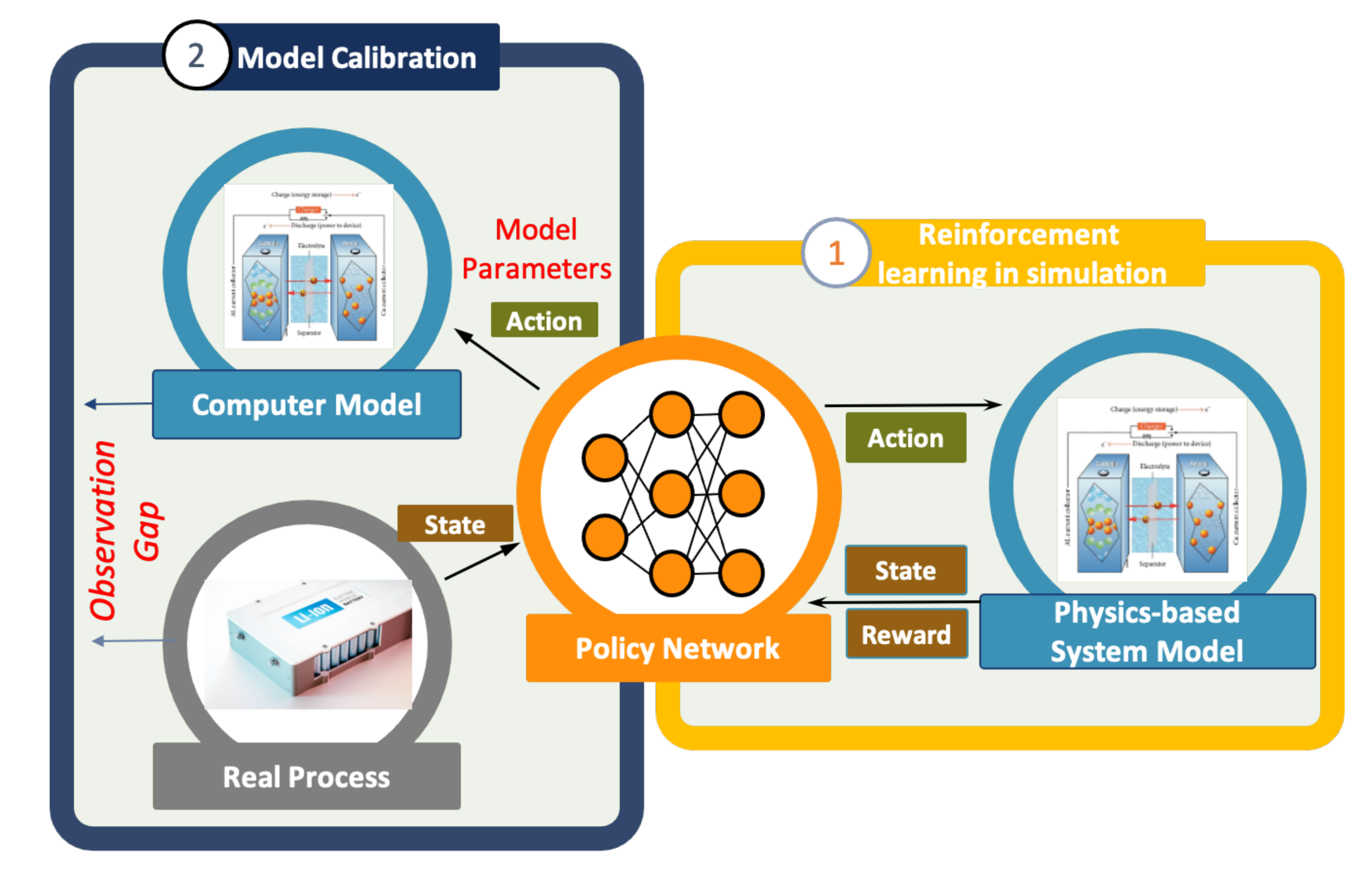
Figure 1. Model calibration: Part (1): the policy network is trained by interacting with the system model. Part (2): the policy network acts as a calibrator at the test time.
Energies 14 01361 g001
Figure 2. Single parameter inference for Qmax and Ro using RL. Degradation trajectories from left to right represent increasing input load condition.
Energies 14 01361 g002
Figure 3. Two parameter inference for Qmax and Ro using RL. For each Qmax trajectory on the left we try multiple degradation values for Ro on the right.
Energies 14 01361 g003
Table 1. Parameter inference (normalized root mean squared error (normalized RMSE) in % for different methods). Single parameter = vary only one parameter (either Q m a x or R o ) at a time. Multi parameter = vary both parameters simultaneously. RL-LAC = reinforcement learning Lyapunov-based actor–critic; UKF = unscented Kalman filter.
MethodSingle ParameterMulti Parameter
QmaxRoQmaxRo
RL-LAC (ours)5.162.078.391.51
UKF19.914.0819.757.54
Direct Mapping0.0110.21.862.5
Table 2. Inference times of a single calibration step for different methods.
Method
RL-LACUKFDirect Mapping
Time (ms)1.994.550.29
Publisher’s Note: MDPI stays neutral with regard to jurisdictional claims in published maps and institutional affiliations.